Semi-fermionic representation for spin systems under equilibrium and non-equilibrium conditions

Abstract

We present a general derivation of semi-fermionic representation for spin operators in terms of a bilinear combination of fermions in real and imaginary time formalisms. The constraint on fermionic occupation numbers is fulfilled by means of imaginary Lagrange multipliers resulting in special shape of quasiparticle distribution functions. We show how Schwinger-Keldysh technique for spin operators is constructed with the help of semi-fermions. We demonstrate how the idea of semi-fermionic representation might be extended to the groups possessing dynamic symmetries (e.g. singlet/triplet transitions in quantum dots). We illustrate the application of semi-fermionic representations for various problems of strongly correlated and mesoscopic physics.


PACS numbers: 71.27.+a, 75.20.Hr

Introduction

It is known that spin operators satisfy neither Fermi nor Bose commutation relations. For example, the Pauli matrices for $S=1/2$ operator commute on different sites and anticommute on the same site. The commutation relations for spins are determined by $SU(2)$ algebra, leading to the absence of a Wick theorem for the generators. To avoid this difficulty and construct a diagrammatic technique and path integral representation for spin systems various approaches have been used. The first class of approaches is based on representation of spins as bilinear combination of Fermi or Bose operators [1]-[7], whereas the representations belonging to the second class deal with more complex objects like, e.g. the Hubbard [8] and supersymmetric [9] operators, the nonlinear sigma model [10] etc. However, in all cases the fundamental problem which is at the heart of the difficulty is the local constraint problem. To illustrate it, let’s consider e.g., first class of representations. Introducing the auxiliary Fermi or Bose fields makes the dimensionality of the Hilbert space, where these operators act, greater than the dimensionality of the Hilbert space for the spin operators. As a result, the spurious unphysical states should be excluded from the consideration which leads in turn to some restrictions (constraints) on bilinear combinations of Fermi/Bose operators, resulting in substantial complication of corresponding rules of the diagrammatic technique. The representations from the second class suffer from the same kind of problem, transformed either into a high nonlinearity of resulting model (non-linear sigma model) or hierarchical structure of perturbation series in the absence of Wick theorem (Hubbard operators). The exclusion of double occupied and empty states for a $S=1/2$ impurity interacting with conduction electron bath (single impurity Kondo model), is controlled by fictitious chemical potential (Lagrange multiplier) of Abrikosov pseudofermions [5]. At the end of calculations this “chemical potential” $\lambda$ should be put $\lambda\to-\infty$ to “freeze out” all unphysical states. In other words, there exists an additional $U(1)$ gauge field which freezes the charge fluctuations associated with this representation. The method works for dilute systems where all the spins can be considered independently. Unfortunately, attempts to generalize this technique to the lattice of spins results in the replacement of the local constraint (the number of particles on each site is fixed) by the so-called global constraint where the number of particles is fixed only on an average for the whole crystal. There is no reason to believe that such an approximation is a good starting point for the description of the strongly correlated systems. Another possibility to treat the local constraint rigorously is based on Majorana fermion representation. In this case fermions are “real” and corresponding gauge symmetry is $Z_{2}$. The difficulty with this representation is mostly related to the physical regularization of the fluctuations associated with the discrete symmetry group.

An alternative approach for spin Hamiltonians, free from local constraint problem, has been proposed in the pioneering paper of Popov and Fedotov [11]. Based on the exact fermionic representation for $S=1/2$ and $S=1$ operators, where the constraint is controlled by purely imaginary Lagrange multipliers, these authors demonstrated the power and simplification of the corresponding Matsubara diagram technique. The semi-fermionic representation (we discuss the meaning of this definition in the course of our paper) used by Popov and Fedotov is neither fermionic, nor bosonic, but reflects the fundamental Pauli nature of spins. The goal of this paper is to give a brief introduction to a semi-fermionic (SF) approach. A reader can find many useful technical details, discussion of mathematical aspects of semi-fermionic representation and its application to various problems in the original papers [11]-[24]. However, we reproduce the key steps of important derivations contained in [19],[20] in order to make the reader’s job easier.

The manuscript is organized as follows: in Section I, the general concept of semi-fermions is introduced. We begin with the construction of the SF formalism for the fully antisymmetric representation of $SU(N)$ group and the fully symmetric SF representation of $SU(2)$ group using the imaginary-time (Matsubara) representation. We show a “bridge” between different representations using the simplest example of $S=1$ in $SU(2)$ and discuss the SF approach for $SO(4)$ group. Finally, we show how to work with semi-fermions in real-time formalism and construct the Schwinger-Keldysh technique for SF. In this section, we will mostly follow original papers by the author [12], [19]. The reader acquainted with semi-fermionic technique can easily skip this section. In Section II, we illustrate the applications of SF formalism for various problems of condensed matter physics, such as ferromagnetic (FM), antiferromagnetic (AFM) and resonance valence bond (RVB) instabilities in the Heisenberg model, Dicke model, large negative - U Hubbard and t-J models, competition between local and non-local correlations in Kondo lattices in the vicinity of magnetic and spin glass critical points, dynamical symmetries in quantum dots, spin chains and ladders. In the Epilogue, we discuss some open questions and perspectives. Necessary information about dynamical groups is contained in Appendix A, the effective models for spin chains are discussed in Appendix B.

1 Semi-fermionic representation

To begin with, we briefly reproduce the arguments contained in the original paper of Popov and Fedotov. Let’s assume first $S=1/2$. We denote as $H_{\sigma}$ the Hamiltonian of spin system. The standard Pauli matrices can be represented as bilinear combination of Fermi operators as follows:

$$\sigma_{j}^{z}\to a_{j}^{\dagger}a_{j}-b_{j}^{\dagger}b_{j},\;\;\;\;\;\;\sigma_{j}^{+}\to 2a_{j}^{\dagger}b_{j},\;\;\;\;\;\;\;\sigma_{j}^{-}\to 2b_{j}^{\dagger}a_{j}.$$ (1)

on each site $i$ of the lattice. The partition function of the spin problem $Z_{\sigma}$ is given by

$$Z_{\sigma}=Tr\exp(-\beta\hat{H}_{\sigma})=i^{N}Tr\exp(-\beta(\hat{H}_{F}+i\pi\hat{N}_{F}/(2\beta))$$ (2)

where $\hat{H}_{F}$ is the operator obtained from $\hat{H}_{\sigma}$ by the replacement (1) and

$$\hat{N}=\sum_{j=1}^{N}(a^{\dagger}_{j}a_{j}+b^{\dagger}_{j}b_{j})$$ (3)

($N$ is the number of sites in the system and $\beta=1/T$ is inverse temperature). To prove equation (2) we note that the trace over the nonphysical states of the $i$-th site vanishes

$$Tr_{unphys}\exp(-\beta(\hat{H}_{F}+i\pi\hat{N}_{F}/(2\beta))=(-i)^{0}+(-i)^{2}=0$$ (4)

Thus, the identity (2) holds. The constraint of fixed number of fermions $\hat{N}_{j}=1$, is achieved by means of the purely imaginary Lagrange multipliers $\mu=-i\pi/(2\beta)$ playing the role of imaginary chemical potentials of fermions. As a result, the Green’s function

$$G=(i\omega_{F}-\epsilon)^{-1}$$ (5)

is expressed in terms of Matsubara frequencies $\omega_{F}=2\pi T(n+1/4)$ corresponding neither Fermi nor Bose statistics.

For $S=1$ we adopt the representation of $\hat{H}_{\sigma}$ in terms of the 3-component Fermi field:

$$\sigma^{z}_{j}\to a^{\dagger}_{j}a_{j}-b^{\dagger}_{j}b_{j},\;\;\;\;\;\sigma^{+}_{j}\to\sqrt{2}(a_{j}^{\dagger}c_{j}+c_{j}^{\dagger}b_{j}),\;\;\;\;\sigma^{-}_{j}\to\sqrt{2}(c_{j}^{\dagger}a_{j}+b_{j}^{\dagger}c_{j}).$$ (6)

The partition function $Z_{\sigma}$ is given by

$$Z_{\sigma}=Tr(-\beta\hat{H}_{\sigma})=\left(\frac{i}{\sqrt{3}}\right)^{N}Tr\exp(-\beta(\hat{H}_{F}+i\pi\hat{N}_{F}/(3\beta)).$$ (7)

It is easy to note that the states with occupation numbers 0 and 3 cancel each other, whereas states with occupation 1 and 2 are equivalent due to the particle-hole symmetry and thus can be taken into account on an equal footing by proper normalization of the partition function. As a result, the Green’s function in the imaginary time representation is expressed in terms of $\omega_{F}=2\pi T(n+1/3)$ frequencies.

In this section, we show how semi-fermionic (Popov-Fedotov) representation can be derived using the mapping of partition function of the spin problem onto the corresponding partition function of the fermionic problem. The cases of arbitrary N (even) for SU(N) groups and arbitrary S for SU(2) group are discussed.

1.1 SU(N) group

We begin with the derivation of SF representation for SU(N) group. The SU($N$) algebra is determined by the generators obeying the following commutation relations:

$$[\hat{S}^{\beta}_{\alpha,i}\hat{S}^{\rho}_{\sigma j}]=\delta_{ij}(\delta^{\rho}_{\alpha}\hat{S}^{\beta}_{\sigma i}-\delta^{\beta}_{\sigma}\hat{S}^{\rho}_{\alpha i}),$$ (8)

where $\alpha,\beta=1,...,N$. We adopt the definition of the Cartan algebra [25] of the SU($N$) group $\{H_{\alpha}\}=S_{\alpha}^{\alpha}$ similar to the one used in [26], noting that the diagonal generators $S_{\alpha}^{\alpha}$ are not traceless. To ensure a vanishing trace, the diagonal generators should only appear in combinations

$$\sum_{\alpha=1}^{N}s_{\alpha}S_{\alpha}^{\alpha}\quad\mbox{with}\quad\sum_{\alpha=1}^{N}s_{\alpha}=0,$$ (9)

which effectively reduce the number of independent diagonal generators to $N-1$ and the total number of SU($N$) generators to $N^{2}-1$.

In this paper we discuss the representations of SU(N) group determined by rectangular Young Tableau (YT) (see [26] and [19] for details) and mostly concentrate on two important cases of the fully asymmetric (one column) YT and the fully symmetric (one row) YT (see Fig.1).

Figure 1: Rectangular Young tableau to denote a SU($N$) representation (a), single column tableau corresponding to $n_{c}=1$ (b) and single row tableau standing for spin $S=n_{c}/2$ representation of SU(2) group (c).

The generator $\hat{S}^{\alpha}_{\beta}$ may be written as biquadratic form in terms of the Fermi-operators

$$\hat{S}^{\alpha}_{\beta}=\sum_{\gamma}a^{\dagger}_{\alpha\gamma}a^{\beta\gamma}$$ (10)

where the ”color” index $\gamma=1,...,n_{c}$ and the $n_{c}(n_{c}+1)/2$ constraints

$$\sum_{\alpha=1}^{N}a^{\dagger}_{\alpha\gamma_{1}}a^{\alpha\gamma_{2}}=\delta_{\gamma_{1}}^{\gamma_{2}}m$$ (11)

restrict the Hilbert space to the states with $m*n_{c}$ particles and ensure the characteristic symmetry in the color index $a$. Here $m$ corresponds to the number of rows in rectangular Young Tableau whereas $n_{c}$ stands for the number of columns. The antisymmetric behavior with respect to $\alpha$ is a direct consequence of the fermionic representation.

Let us consider the partition function for the Hamiltonian, expressed in terms of SU($N$) generators

$$Z_{S}=Tr\exp(-\beta H_{S})=Tr^{\prime}\exp(-\beta H_{F})$$ (12)

where $Tr^{\prime}$ denotes the trace taken with constraints (11). As it is shown in [19], the partition function of $SU(N)$ model is related to partition function of corresponding fermion model through the following equation:

$$Z_{S}=\int\prod_{j}d\mu(j)P(\mu(j))Tr\exp\left(-\beta(H_{F}-\mu(j)n_{F})\right)=$$ (13)

$$=\int\prod_{j}d\mu(j)P(\mu(j))Z_{F}(\mu(j))$$

here $P(\mu_{j})$ is a distribution function of imaginary Lagrange multipliers. We calculate $P(\mu_{j})$ explicitly using constraints (11).

We use the path integral representation of the partition function

$$Z_{S}/Z_{S}^{0}=\int\prod_{j}d\mu(j)P(\mu(j))\exp({\cal A})/\int\prod_{j}d\mu(j)P(\mu(j))\exp({\cal A}_{0})$$ (14)

where the actions ${\cal A}$ and ${\cal A}_{0}$ are determined by

$${\cal A}={\cal A}_{0}-\int_{0}^{\beta}d\tau H_{F}(\tau),\;\;\;{\cal A}_{0}=\sum_{j}\sum_{k=1}^{N}\int_{0}^{\beta}d\tau\bar{a}_{k}(j,\tau)(\partial_{\tau}+\mu(j))a_{k}(j,\tau)$$ (15)

and the fermionic representation of SU($N$) generators (10) is applied.

Let us first consider the case $n_{c}=1$. We denote the corresponding distribution by $P_{N,m}(\mu(j))$, where $m$ is the number of particles in the SU($N$) orbital, or in other words, $1\leq m<N$ labels the different fundamental representations of SU($N$).

$$n_{j}=\sum_{k=1}^{N}\bar{a}_{k}(j)a_{k}(j)=m$$ (16)

To satisfy this requirement, the minimal set of chemical potentials and the corresponding form of $P_{N,m}(\mu(j))$ are to be derived (see Fig.2).

To derive the distribution function, we use the following identity for the constraint (16) expressed in terms of Grassmann variables

$$\delta_{n_{j},m}=\frac{1}{N}\sin\left(\pi(n_{j}-m)\right)/\sin\left(\frac{\pi(n_{j}-m)}{N}\right)$$ (17)

Substituting this identity into (12) and comparing with (14) one gets

$$P_{N,m}(\mu(j))=\frac{1}{N}\sum_{k=1}^{N}\exp\left(\frac{i\pi m}{N}(2k-1)\right)\delta(\mu(j)-\mu_{k}),$$ (18)

where

$$\mu_{k}=-\frac{i\pi T}{N}(2k-1).$$ (19)

Since the Hamiltonian is symmetric under the exchange of particles and holes when the sign of the Lagrange multiplier is also changed simultaneously, we can simplify (18) to

$$P_{N,m}(\mu(j))=\frac{2i}{N}\sum_{k=1}^{\lfloor N/2\rfloor}\sin\left(\pi m\frac{2k-1}{N}\right)\delta(\mu(j)-\mu_{k})$$ (20)

where $\lfloor N/2\rfloor$ denotes the integer part of $N/2$. As shown below, this is the minimal representation of the distribution function corresponding to the minimal set of the discrete imaginary Lagrange multipliers. Another distributions function different from (20) can be constructed when the sum is taken from $k=N/2+1$ to $N$. Nevertheless, this DF is different from (20) only by the sign of imaginary Lagrange multipliers $\tilde{\mu}_{k}=\mu_{k}^{*}=-\mu_{k}$ and thus is supplementary to (20).

Figure 2: Graphical representation of exclusion principle for SU($N$) semi-fermionic representation with even $N$, $n_{c}=1$ (we use $\mu=i\pi T/2$ for SU(2) and $\mu_{1}=i\pi T/4,\;\mu_{2}=3i\pi T/4$ for SU(4)).

Particularly interesting for even $N$ is the case when the SU($N$) orbital is half–filled, $m=N/2$. Then all Lagrange multipliers carry equal weight

$$P_{N,N/2}(\mu(j))=\frac{2i}{N}\sum_{k=1}^{N/2}(-1)^{k+1}\delta\left(\mu(j)-\mu_{k}\right).$$ (21)

Taking the limit $N\to\infty$ one may replace the summation in expression (21) in a suitable way by integration. Note, that while taking $N\to\infty$ and $m\to\infty$ limits, we nevertheless keep the ratio $m/N=1/2$ fixed. Then, the following limiting distribution function can be obtained:

$$P_{N,N/2}(\mu(j))\stackrel{{\scriptstyle N\to\infty}}{{\longrightarrow}}\frac{\beta}{2\pi i}\exp\left(-\beta\mu(j)\frac{N}{2}\right)$$ (22)

resulting in the usual continuous representation of the local constraint for the simplest case $n_{c}=1$

$$Z_{S}=Tr(\exp\left(-\beta H_{F}\right)\delta\left(n_{j}-\frac{N}{2}\right)$$ (23)

We note the obvious similarity of the limiting DF (22) with the Gibbs canonical distribution provided that the Wick rotation from the imaginary axis of the Lagrange multipliers $\mu$ to the real axis of energies $E$ is performed and thus $\mu(j)N/2$ has a meaning of energy.

Up to now, the representation we discussed was purely fermionic and expressed in terms of usual Grassmann variables when the path integral formalism is applied. The only difference from slave fermionic approach is that imaginary Lagrange multipliers are introduced to fulfill the constraint. Nevertheless, by making the replacement

$$a_{k}(j,\tau))\to a_{k}(j,\tau)\exp\left(\frac{i\pi\tau}{\beta}\frac{2k-1}{N}\right),\;\;\;\bar{a}_{k}(j,\tau)\to\bar{a}_{k}(j,\tau)\exp\left(-\frac{i\pi\tau}{\beta}\frac{2k-1}{N}\right)$$ (24)

we arrive at the generalized Grassmann (semi-fermionic) boundary conditions

$$a_{k}(j,\beta)=a_{k}(j,0)\exp\left(i\pi\frac{2k-1}{N}\right),\;\;\;\bar{a}_{k}(j,\beta)=\bar{a}_{k}(j,0)\exp\left(-i\pi\frac{2k-1}{N}\right)$$ (25)

This leads to a temperature diagram technique for the Green’s functions

$${\cal G}^{\alpha\beta}(j,\tau)=-\langle T_{\tau}a_{\alpha}(j,\tau)\bar{a}_{\beta}(j,0)\rangle$$ (26)

of semi-fermions with Matsubara frequencies different from both Fermi and Bose representations (see Fig.3).

Figure 3: The minimal set of Matsubara frequencies for a) $SU(N)$ representation with even $N$/ $SU(2)$ representation for half-integer value of the spin. b) $SU(2)$ representation for integer values of the spin and $l=1$.

The exclusion principle for this case is illustrated on Fig.2, where the $S=1/2$ representation for the first two groups SU(2) and SU(4) are shown. The first point to observe is that the spin Hamiltonian does not distinguish the $n$ particle and the $n$ hole (or $N-n$ particle) subspace. Eq. (19) shows that the two phase factors $\exp(\beta\mu n)$ and $\exp(\beta\mu(N-n))$ accompanying these subspaces in Eq. (20) add up to a purely imaginary value within the same Lagrange multiplier, and the empty and the fully occupied states are always cancelled. In the case of $N\geq 4$, where we have multiple Lagrange multipliers, the distribution function $P(\mu)$ linearly combines these imaginary prefactors to select out the desired physical subspace with particle number $n=m$.

In Fig.2, we note that on each picture, the empty and fully occupied states are cancelled in their own unit circle. For SU(2) there is a unique chemical potential $\mu=\pm i\pi T/2$ which results in the survival of single occupied states. For SU(4) there are two chemical potentials (see also Fig.3). The cancellation of single and triple occupied states is achieved with the help of proper weights for these states in the distribution function whereas the states with the occupation number 2 are doubled according to the expression (21). In general, for SU($N$) group with $n_{c}=1$ there exists $N/2$ circles providing the realization of the exclusion principle.

1.2 SU(2) group

We consider now the generalization of the SU(2) algebra for the case of spin $S$. Here, the most convenient fermionic representation is constructed with the help of a $2S+1$ component Fermi field $a_{k}(j)$ provided that the generators of SU(2) satisfy the following equations:

$$S^{+}=\sum_{k=-S}^{S-1}\sqrt{S(S+1)-k(k+1)}a^{\dagger}_{k+1}(j)a_{k}(j),$$

$$S^{-}=\sum_{k=-S+1}^{S}\sqrt{S(S+1)-k(k-1)}a^{\dagger}_{k-1}(j)a_{k}(j),$$

$$S^{z}=\sum_{k=-S}^{S}ka^{\dagger}_{k}(j)a_{k}(j)$$ (27)

such that $dimH_{F}=2^{2S+1}$ whereas the constraint reads as follows

$$n_{j}=\sum_{k=-S}^{k=S}a^{\dagger}_{k}(j)a_{k}(j)=l=1$$ (28)

Following the same routine as for SU($N$) generators and using the occupancy condition to have $l=1$ (or $2S$) states of the $(2S+1)$ states filled, one gets the following distribution function, after using the particle–hole symmetry of the Hamiltonian $H_{S}$:

$$P_{2S+1,1}(\mu(j))=\frac{2i}{2S+1}\sum_{k=1}^{\lfloor S+1/2\rfloor}\sin\left(\pi\frac{2k-1}{2S+1}\right)\delta(\mu(j)-\mu_{k})$$ (29)

where the Lagrange multipliers are $\mu_{k}=-i\pi T(2k-1)/(2S+1)$ and $k=1,...,\lfloor S+1/2\rfloor$, similarly to Eq.(19).

In the particular case of the SU(2) model for some chosen values of spin $S$ the distribution functions are given by the following expressions

$$P_{2,1}(\mu(j))=i\;\delta\left(\mu(j)+\frac{i\pi T}{2}\right)$$

for $S=1/2$

$$P_{3,1}(\mu(j))=P_{3,2}(\mu(j))=\frac{i}{\sqrt{3}}\;\delta\left(\mu(j)+\frac{i\pi T}{3}\right)$$

for $S=1$.

This result corresponds to the original Popov-Fedotov description restricted to the $S=1/2$ and $S=1$ cases.

Figure 4: Graphical representation of exclusion principle for SU(2) semi-fermionic representation for $S=1$ and $S=2$. For any arbitrary integer value of spin there exists $S$ circle diagrams corresponding to the $S$ different chemical potentials and providing the realization of the exclusion principle.

We present as an example some other distribution functions obtained according to general scheme considered above:

$$P_{4,1}(\mu)=P_{4,3}(\mu)=$$

$$=\frac{i\sqrt{2}}{4}\left(\delta(\mu+\frac{i\pi T}{4})+\delta(\mu+\frac{3i\pi T}{4})\right)$$

for $S=3/2$, SU(2) and

$$P_{4,2}(\mu)=\frac{i}{2}\left(\delta(\mu+\frac{i\pi T}{4})-\delta(\mu+\frac{3i\pi T}{4})\right)$$

for effective spin ”$S=1/2$”, SU(4),

$$P_{5,1}(\mu)=P_{5,4}(\mu)=$$

$$=\frac{i}{\sqrt{10}}\left(\sqrt{1-\frac{1}{\sqrt{5}}}\;\;\delta(\mu+\frac{i\pi T}{5})+\sqrt{1+\frac{1}{\sqrt{5}}}\;\;\delta(\mu+\frac{3i\pi T}{5})\right)$$

for $S=2$, $SU(2)$ etc.

A limiting distribution function corresponding to Eq. (22) for the constraint condition with arbitrary $l$ is found to be

$$P_{\infty,l}(\mu(j))\stackrel{{\scriptstyle S\to\infty}}{{\longrightarrow}}\frac{\beta}{2\pi i}\exp(-\beta l\mu(j)).$$ (30)

For the case $l=m=N/2\to\infty$ and $S=(N-1)/2\to\infty$ the expression for the limiting DF $P_{\infty,l}(\mu(j))$ coincides with (23). We note that in $S\to\infty$ (or $N\to\infty$) limit, the continuum “chemical potentials” play the role of additional U(1) fluctuating field whereas for finite $S$ and $N$ they are characterized by fixed and discrete values.

When $S$ assumes integer values, the minimal fundamental set of Matsubara frequencies is given by the table in Fig.3.

The exclusion principle for SU(2) in the large spin limit can be also understood with the help of Fig.2 and Fig.4. One can see that the empty and the fully occupied states are cancelled in each given circle similarly to even-$N$ SU($N$) algebra. The particle-hole (PH) symmetry of the representation results in an equivalence of single occupied and $2S$ occupied states whereas all the other states are cancelled due to proper weights in the distribution function (29). In accordance with PH symmetry being preserved for each value of the chemical potential all circle diagrams (see Fig.3, Fig.5) are invariant with respect to simultaneous change $\mu\leftrightarrow-\mu$ and $n_{particle}\leftrightarrow n_{holes}$.

1.3 Semi-fermionic representation of $SO(N)$ group

In this chapter we show the way of generalization of semi-fermionic representation to the dynamical algebras $o(4)$ and $o(5)$ (see Appendix A). Like in the case of pure spin operators, these representations should preserve all kinematical constraints.

The first step to derive semi-fermionic representation for SO(4) group is based on the local isomorphism of $SO(4)$ and $SU(2)\times SU(2)$.

We start with $n=4$ - field representation of $SU(2)$ group (10)

$$(a_{11},~{}a_{12},~{}a_{21},~{}a_{22})$$ (31)

There are two diagonal and two off-diagonal constraints (11) which read as follows:

$$a^{\dagger}_{11}a_{11}+a^{\dagger}_{21}a_{21}=1,\;\;\;\;a^{\dagger}_{12}a_{12}+a^{\dagger}_{22}a_{22}=1,$$ (32)

$$a^{\dagger}_{11}a_{12}+a^{\dagger}_{21}a_{22}=0,\;\;\;\;a^{\dagger}_{12}a_{11}+a^{\dagger}_{22}a_{21}=0,$$ (33)

and generators of $SU(2)$ group are given by

$$S^{-}=S_{2}^{1}=a^{\dagger}_{11}a_{21}+a^{\dagger}_{12}a_{22},\;\;\;\;S^{+}=S_{1}^{2}=a^{\dagger}_{21}a_{11}+a^{\dagger}_{22}a_{12}$$

$$2S^{z}=S_{2}^{2}-S_{1}^{1}=a^{\dagger}_{21}a_{21}+a^{\dagger}_{22}a_{22}-a^{\dagger}_{11}a_{11}-a^{\dagger}_{12}a_{12}$$ (34)

Combining definition (34) with constraint (33) we reach the following equations:

$$S^{-} = a^{\dagger}_{11}(a_{21}+a_{12})+(a^{\dagger}_{12}+a^{\dagger}_{21})a_{22},$$

$$S^{+} = (a^{\dagger}_{21}+a^{\dagger}_{12})a_{11}+a^{\dagger}_{22}(a_{12}+a_{21}),$$

$$S^{z} = a^{\dagger}_{22}a_{22}-a^{\dagger}_{11}a_{11}$$ (35)

Therefore, we conclude that the antisymmetric (singlet) combination $a_{12}-a_{21}$ does not enter the expression for spin $S=1$ operators. Thus, three (out of four) component Fermi-field is sufficient for the description of $S=1$ $SU(2)$ representation in agreement with (27). Defining new fields as follows

$$a_{11}=f_{-1},\;\;\;\;a_{22}=f_{1},\;\;\;\;\;\frac{1}{\sqrt{2}}(a_{12}+a_{21})=f_{0},\;\;\;\;\;\;\frac{1}{\sqrt{2}}(a_{12}-a_{21})=f_{s}.$$ (36)

where fermions $f_{1},f_{0},f_{-1}$ stand for $S^{z}=1,0-1$ projections of the triplet state and fermion $s$ determines the singlet state, we come to standard $S=1$ $SU(2)$ representation

$$S^{+}=\sqrt{2}(f_{0}^{\dagger}f_{-1}+f^{\dagger}_{1}f_{0}),\;\;\;\;\;S^{-}=\sqrt{2}(f^{\dagger}_{-1}f_{0}+f_{0}^{\dagger}f_{1}),\;\;\;\;\;S_{z}=f^{\dagger}_{1}f_{1}-f^{\dagger}_{-1}f_{-1},$$ (37)

with the constraint

$$n_{1}+n_{0}+n_{-1}+n_{s}=2$$ (38)

where $n_{\alpha}=f^{\dagger}_{\alpha}f_{\alpha}$.

The constraint (38) transforms to a standard $SU(2)$ $S=1$ constraint (43) in both cases $n_{s}=0$ and $n_{s}=1$ since there is no singlet/triplet mixing allowed by $SU(2)$ algebra.

To demonstrate the transformation of the local constraint let’s first consider the case $n_{s}=0$. The constraint reads as follows

$$n_{1}+n_{0}+n_{-1}=2S\;\;\;\;\;\iff\;\;\;\;\;\;\;{\bf S}^{2}=S(S+1).$$ (39)

On the other hand, the states with $2S$ occupation are equivalent to the states with single occupation due to particle-hole symmetry. Thus, the constraint (38) might be written as

$$\tilde{n}_{1}+\tilde{n}_{0}+\tilde{n}_{-1}=1$$ (40)

where $\tilde{n}_{\alpha}=1-n_{\alpha}$. The latter case corresponds to $n_{s}=1$.

The singlet/triplet mixing is allowed for $SO(4)$ group. This mixing is described in terms of 3 additional generators responsible for transitions between singlet and triplet (see Appendix A). Using 4-component auxiliary fermions $f_{\lambda}$, where $\lambda=-1,0,1,s$ and matrix form of generators (163) we represent $R$ - generators of $SO(4)$ as follows

$$R^{+} = \sqrt{2}(f^{\dagger}_{1}f_{s}-f_{s}^{\dagger}f_{-1}),\;\;\;\;R^{-}=\sqrt{2}(f_{s}^{\dagger}f_{1}-f^{\dagger}_{-1}f_{s}),\;\;\;\;R^{z}=-(f_{0}^{\dagger}f_{s}+f_{s}^{\dagger}f_{0}).$$

with the only constraint

$$n_{1}+n_{0}+n_{-1}+n_{s}=1,\;\;\;\;\;\iff\;\;\;\;\;\;\;{\bf S}^{2}+{\bf R}^{2}=3$$ (41)

whereas the orthogonality condition ${\bf S}\cdot{\bf R}={\bf R}\cdot{\bf S}=0$ is fulfilled automatically. The constraint (41) is respected by means of introducing real chemical potential $\lambda\to\infty$ for Abrikosov’s auxiliary fermions or imaginary chemical potentials $\mu_{t}=-i\pi T/3$ for Popov-Fedotov semi-fermion.

The fermionic representation of $SO(5)$ group is easily constructed by use semi-fermionic representation and is characterized by 5-vector ${\bf q}^{T}=(f_{-1}^{\dagger}f_{0}^{\dagger},f_{1}^{\dagger},f_{s}^{\dagger},f_{r}^{\dagger})$

$$S^{+} = \sqrt{2}(f_{0}^{\dagger}f_{-1}+f^{\dagger}_{1}f_{0}),\;\;\;\;S^{z}=f^{\dagger}_{1}f_{1}-f^{\dagger}_{-1}f_{-1},$$

$$R^{+} = \sqrt{2}(f^{\dagger}_{1}f_{s}-f_{s}^{\dagger}f_{-1}),\;\;\;\;R^{z}=-(f_{0}^{\dagger}f_{s}+f_{s}^{\dagger}f_{0}),$$

$$P^{+} = \sqrt{2}(f^{\dagger}_{1}f_{r}-f_{r}^{\dagger}f_{-1}),\;\;\;\;P^{z}=-(f_{0}^{\dagger}f_{r}+f_{r}^{\dagger}f_{0}).$$ (42)

and

$$A=i(f_{r}^{\dagger}f_{s}-f_{s}^{\dagger}f_{r})$$

The constraint

$$n_{1}+n_{0}+n_{-1}+n_{s}+n_{r}=1$$ (43)

is respected either by real infinite chemical potential (Abrikosov pseudofermions) or by set of complex chemical potentials (semi-fermions). We do not present here ten $5\times 5$ matrices characterizing $SO(5)$ representation to save a space. The reader can easily construct them using representations (42). There exists also a bosonic representation based on Schwinger bosons which might be derived by the method similar to used above for $SO(4)$ group. The representations of higher $SO(n)$ groups can be constructed in a similar fashion.

Kinematic constraints imposed on auxiliary fermions and bosons is in strict compliance with the Casimir and orthogonality constraints in spin space. Accordingly, the number of fermionic and bosonic fields reproduces the dimensionality of spin space reduced by these constraints. We have seen that the 6-D space of generators of $SO(4)$ group is reduced to D=4. Then the minimal (unconstraint) fermionic representation for this group should contain two $U(1)$ fermions. This means that the representation (1.3) is not minimal. Apparently, the best way to find such representation is to use Jordan-Wigner-like transformation [10]. The exact form of Jordan-Wigner transformation for $SO(4)$ group was recently reported in [27]. The same kind of arguments applied to $SO(5)$ group tells us that the spinor field should contain seven components. This means that the 3-color U(1) fermionic representation should be completed by one more real (Majorana) fermion, and this fact points to one more hidden $Z_{2}$ symmetry [10].

1.4 Real-time formalism

We discuss finally the real-time formalism based on the semi-fermionic representation of SU($N$) generators. This approach is necessary for treating the systems out of equilibrium, especially for many component systems describing Fermi (Bose) quasiparticles interacting with spins. The real time formalism [28], [29] provides an alternative approach for the analytical continuation method for equilibrium problems allowing direct calculations of correlators whose analytical properties as function of many complex arguments can be quite cumbersome.

To derive the real-time formalism for SU($N$) generators we use the path integral representation along the closed time Keldysh contour (see Fig.5).

Figure 5: The Keldysh contour going from $-\infty\to\infty\to-\infty$ in real time. The boundary conditions on the imaginary time segment determine the generalized distribution functions for quasiparticles.

Following the standard route [30], we can express the partition function of the problem containing SU($N$) generators as a path integral over Grassmann variables $\psi_{l}=(a_{l,1}(j),...,a_{l,N}(j))^{T}$ where $l=1,2$ stands for upper and lower parts of the Keldysh contour, respectively,

$${\cal Z}/{\cal Z}_{0}=\int D\bar{\psi}D\psi\exp(i{\cal A})/\int D\bar{\psi}D\psi\exp(i{\cal A}_{0})$$ (44)

where the actions ${\cal A}$ and ${\cal A}_{0}$ are taken as an integral along the closed-time contour $C_{t}+C_{\tau}$ which is shown in Fig.5. The contour is closed at $t=-\infty+i\tau$ since $\exp(-\beta H_{0})=T_{\tau}\exp\left(-\int_{0}^{\beta}H_{0}d\tau\right).$ We denote the $\psi$ fields on upper and lower sides of the contour $C_{t}$ as $\psi_{1}$ and $\psi_{2}$ respectively. The fields $\Psi$ stand for the contour $C_{\tau}$. These fields provide the matching conditions for $\psi_{1,2}$ and are excluded from the final expressions. Taking into account the semi-fermionic boundary conditions for generalized Grassmann fields (25) one gets the matching conditions for $\psi_{1,2}$ at $t=\pm\infty$,

$$\psi^{\mu}_{1,\alpha}|_{k}(-\infty)=\exp\left(i\pi\frac{2k-1}{N}\right)\psi^{\mu}_{2,\alpha}|_{k}(-\infty),$$

$$\psi^{\mu}_{1,\alpha}|_{k}(+\infty)=\psi^{\mu}_{2,\alpha}|_{k}(+\infty)$$ (45)

for $k=1,...,\lfloor N/2\rfloor$ and $\alpha=1,...,N$. The correlation functions can be represented as functional derivatives of the generating functional

$$Z[\eta]={\cal Z}_{0}^{-1}\int D\bar{\psi}D\psi\exp\left(i{\cal A}+i\oint_{C}dt(\bar{\eta}\sigma^{z}\psi+\bar{\psi}\sigma^{z}\eta)\right)$$ (46)

where $\eta$ represents sources and the $\sigma^{z}$ matrix stands for ”causal” and ”anti-causal” orderings along the contour.

The on-site Green’s functions (GF) which are matrices of size $2N\times 2N$ with respect to both Keldysh (lower) and spin-color (upper) indices are given by

$$G_{\mu\nu}^{\alpha\beta}(t,t^{\prime})=-i\frac{\delta}{i\delta\bar{\eta}_{\mu}^{\alpha}(t)}\frac{\delta}{i\delta\eta_{\nu}^{\beta}(t^{\prime})}Z[\eta]|_{\bar{\eta},\eta\to 0}.$$ (47)

To distinguish between imaginary-time (26) and real-time (47) GF’s, we use different notations for Green’s functions in these representations.

After a standard shift-transformation [30] of the fields $\psi$ the Keldysh GF of free semi-fermions assumes the form

$$G_{0}^{\alpha}(\epsilon)=G^{R,\alpha}_{0}\left(\begin{array}[]{cc}1-f_{\epsilon}&-f_{\epsilon}\\ 1-f_{\epsilon}&-f_{\epsilon}\end{array}\right)-G^{A,\alpha}_{0}\left(\begin{array}[]{cc}-f_{\epsilon}&-f_{\epsilon}\\ 1-f_{\epsilon}&1-f_{\epsilon}\end{array}\right),$$ (52)

where the retarded and advanced GF’s are

$$G^{(R,A)\alpha}_{0}(\epsilon)=(\epsilon\pm i\delta)^{-1},\quad f_{\epsilon}=f^{(N,k)}(\epsilon),$$ (53)

with equilibrium distribution functions

$$f^{(N,k)}(\epsilon)=T\sum_{n}\frac{e^{i\omega_{n_{k}}\tau|_{+0}}}{i\omega_{n_{k}}-\epsilon}=\frac{1}{e^{i\pi(2k-1)/N}\exp(\beta\epsilon)+1}.$$ (54)

A straightforward calculation of $f^{(N,k)}$ for the case of even $N$ leads to the following expression

$$f^{(N,k)}(\epsilon)=\frac{\displaystyle\sum_{l=1}^{N}(-1)^{l-1}\exp\left(\beta\epsilon(N-l)\right)\exp\left(-\frac{i\pi l(2k-1)}{N}\right)}{\exp(N\beta\epsilon)+1},$$ (55)

where $k=1,...,N/2.$ The equilibrium distribution functions (EDF) $f^{(2S+1,k)}$ for the auxiliary Fermi-fields representing arbitrary $S$ for $SU(2)$ algebra are given by

$$f^{(2S+1,k)}(\epsilon)=\frac{\displaystyle\sum_{l=1}^{2S+1}(-1)^{l-1}\exp\left(\beta\epsilon(2S+1-l)\right)\exp\left(-\frac{i\pi(2k-1)}{2S+1})\right)}{\exp((2S+1)\beta\epsilon)+(-1)^{2S+1}}$$ (56)

for $k=1,...,\lfloor S+1/2\rfloor$. Particularly simple are the cases of $S=1/2$ and $S=1$,

$$f^{(2,1)}(\epsilon)=n_{F}(2\epsilon)-i\frac{1}{2\cosh(\beta\epsilon)}$$ (57)

$$f^{(3,1)}(\epsilon)=\frac{1}{2}n_{B}(\epsilon)-\frac{3}{2}n_{B}(3\epsilon)-i\sqrt{3}\frac{\sinh(\beta\epsilon/2)}{\sinh(3\beta\epsilon/2)}$$ (58)

Here, the standard notations for Fermi/Bose distribution functions $n_{F/B}(\epsilon)=[\exp(\beta\epsilon)\pm 1]^{-1}$ are used. For $S=1/2$ the semi-fermionic EDF satisfies the obvious identity $|f^{(2,1)}(\epsilon)|^{2}=n_{F}(2\epsilon)$.

In general the EDF for half-integer and integer spins can be expressed in terms of Fermi and Bose EDF respectively. We note that since auxiliary Fermi fields introduced for the representation of SU($N$) generators do not represent the true quasiparticles of the problem, helping only to treat properly the constraint condition, the distribution functions for these objects in general do not have to be real functions. Nevertheless, one can prove that the imaginary part of the EDF does not affect the physical correlators and can be eliminated by introducing an infinitesimally small real part for the chemical potential. In spin problems, a uniform/staggered magnetic field usually plays the role of such real chemical potential for semi-fermions.

2 Application of semi-fermionic representation for strongly correlated systems

In this Section we illustrate some of the applications of SF representation for various problems of strongly correlated physics.

2.1 Heisenberg model: FM, AFM and RVB

The effective nonpolynomial action [31, 32] for Heisenberg model with ferromagnetic (FM) coupling has been investigated in [11]. The model with antiferromagnetic (AFM) interaction has been considered by means of semi-fermionic representation in [17] and [18] (magnon spectra) and in [12] for resonance valence bond (RVB) excitations. The Hamiltonian considered is given as

$$H_{int}=-\sum_{<ij>}J_{ij}\left(\vec{S}_{i}\vec{S}_{j}-\frac{1}{4}\right)$$ (59)

• Ferromagnetic coupling $J=I_{FM}>0$

The exchange $\vec{S}_{i}\vec{S}_{j}$ is represented as four-semi-fermion interaction. Applying the Hubbard-Stratonovich transformation by the local vector field $\vec{\Phi}_{i}(\tau)$ the effective nonpolynomial action is obtained in terms of vector c-field. The FM phase transition corresponds to the appearance at $T\leq T_{c}$ of the nonzero average $\langle\Phi^{z}(q=0,0)\rangle$ which stands for the nonzero magnetization, or in other words, corresponds to the Bose condensation of the field $\Phi^{z}$.

$$\Phi^{z}(\vec{k},\omega)={\cal M}(\beta N)^{1/2}\delta_{\vec{k},0}\delta_{\omega,0}+\tilde{\Phi}^{z}(\vec{k},\omega).$$ (60)

In one loop approximation the standard molecular field equation can be reproduced

$${\cal M}=I_{FM}(0)\tanh(\beta{\cal M}/2).$$ (61)

The saddle point (mean-field) effective action is given by well-known expression

$${\cal A}_{0}[{\cal M}]=-N\left[\frac{\beta{\cal M}^{2}}{4I_{M}(0)}-\ln\left(2\cosh\left(\frac{\beta{\cal M}}{2}\right)\right)\right],$$ (62)

and the free energy per spin $f_{0}$ is determined by the standard equation:

$$\beta f_{0}=-\ln Z_{S}=\frac{\beta{\cal M}^{2}}{4I_{M}(0)}-\ln\left(2\cosh\left(\frac{\beta{\cal M}}{2}\right)\right)$$ (63)

Calculation of the second variation of ${\cal A}_{eff}$ gives rise to the following expression

$$\delta{\cal A}_{eff}=-\frac{1}{4}\sum_{\vec{k}}\Phi^{z}(\vec{k},0)\left[I_{M}^{-1}(\vec{k})-\frac{\beta}{2\cosh^{2}(\beta\Omega)}\right]\Phi^{z}(\vec{k},0)-$$

$$-\frac{1}{4}\sum_{\vec{k},\omega\neq 0}I_{M}^{-1}(\vec{k})\Phi^{z}(\vec{k},\omega)\Phi^{z}(\vec{k},\omega)-$$

$$-\sum_{\vec{k},\omega}\Phi^{+}(\vec{k},\omega)\left[I_{M}^{-1}(\vec{k})-\frac{\tanh(\beta\Omega)}{2\Omega-i\omega}\right]\Phi^{-}(\vec{k},\omega)$$ (64)

where $\Omega=(g\mu_{B}H+{\cal M})/2$. The magnon spectrum ($T\leq T_{c}$) is determined by the poles of $\langle\Phi^{+}\Phi^{-}\rangle$ correlator, $\omega=\lambda{\bf k}^{2}$.

• Antiferromagnetic coupling $J=I_{AFM}<0$. Néel solution

The AFM transition corresponds to formation of the staggered condensate

$$\Phi^{z}(\vec{k},\omega)={\cal N}(\beta N)^{1/2}\delta_{\vec{k},\vec{Q}}\delta_{\omega,0}+\tilde{\Phi}^{z}(\vec{k},\omega)$$ (65)

The one-loop approximation leads to standard mean-field equations for the staggered magnetization

$${\cal N}=-I_{AFM}(Q)\tanh(\beta{\cal N}/2),$$

$${\cal A}_{0}[{\cal N}]=N\left[\frac{\beta{\cal N}^{2}}{4I_{AFM}(Q)}+\ln\left(2\cosh\left(\frac{\beta{\cal N}}{2}\right)\right)\right].$$ (66)

After taking into account the second variation of ${\cal A}_{eff}$, the following expression for the effective action is obtained [(see e.g. [17],[18]):

$$\delta{\cal A}_{eff}=\frac{1}{4}\sum_{\vec{k}}\Phi^{z}(\vec{k},0)\left[I_{AFM}^{-1}(\vec{k})+\frac{\beta}{2\cosh^{2}(\beta\tilde{\Omega})}\right]\Phi^{z}(\vec{k},0)+$$

$$+\frac{1}{4}\sum_{\vec{k},\omega\neq 0}I_{AFM}^{-1}(\vec{k})\Phi^{z}(\vec{k},\omega)\Phi^{z}(\vec{k},\omega)+$$

$$+\sum_{\vec{k},\omega}\Phi^{+}(\vec{k},\omega)\left[I_{AFM}^{-1}(\vec{k})+\frac{2\tilde{\Omega}\tanh(\beta\tilde{\Omega})}{4\tilde{\Omega}^{2}+\omega^{2}}\right]\Phi^{-}(\vec{k},\omega)-$$

$$-\sum_{\vec{k},\omega}\Phi^{+}(\vec{k}+\vec{Q},\omega)\frac{i\omega}{4\tilde{\Omega}^{2}+\omega^{2}}\Phi^{-}(\vec{k},\omega).$$ (67)

The AFM magnon spectrum $\omega=c|{\bf k}|$.

• Antiferromagnetic coupling. Resonance Valence Bond solution

The four-semi-fermion term in (59) is decoupled by bilocal scalar field $\Lambda_{ij}$. The RVB spin liquid (SL) instability in 2D Heisenberg model corresponds to Bose-condensation of exciton-like pairs of semi-fermions (for simplicity we consider the uniform RVB state):

$$\Delta_{0}=-\sum_{\bf q}\frac{I_{\bf q}}{I_{0}}\tanh\left(\frac{I_{\bf q}\Delta_{0}}{T}\right),$$ (68)

$${\cal A}_{0}=\frac{\beta|I|\Delta_{0}^{2}}{2}-\sum_{\bf q}\ln\left[2\cosh(\beta I_{\bf q}\Delta_{0})\right]$$

where $\Delta_{0}=\Delta({\bf q}=0)$ is determined by the modulus of $\Lambda_{ij}$ field

$$\Lambda_{<ij>}(\vec{R},\;\vec{r})=\Delta(\vec{r})\exp\left(i\vec{r}\vec{A}(\vec{R})\right)$$ (69)

whereas the second variation of $\delta{\cal A}_{eff}$ describes the fluctuations of phase $\Lambda_{ij}$

$${\cal A}_{eff}=\sum_{{\bf k},\omega}A_{\alpha}({\bf k},\omega)\pi^{\alpha\beta}_{{\bf k},\omega}A_{\beta}({\bf k},\omega),$$

$${\Large\pi}^{\alpha\beta}_{{\bf k},\omega}=Tr(p^{\alpha}p^{\beta}(G_{p+k}G_{p}+G_{p+k}G_{p})+\delta_{\alpha\beta}f(I_{\bf p}\Delta_{0}))$$ (70)

The spectrum of excitation in uniform SL is determined by zeros of $\pi^{R}$ and is purely diffusive [33]-[34]. The recent development of application of semi-fermions to low dimensional magnetic systems can be found in [21, 22].

2.2 Dicke model

In this Section we describe the application of semi-fermionic approach to two-level systems interacting with single-mode radiation field (Dicke model). The influence of dissipative environment on two-level system has been extensively studied in spin-boson model [35] (see also a review [36] for coherent effects in mesoscopic few level system, Dicke super and sub-radiance effects). Addressing the reader to above mentioned reviews for discussion of physical implementation of the Dicke model, we discuss in this section only technical aspects related to derivation of its equilibrium (thermodynamical) properties. We closely follow original derivation contained in Popov-Fedotov paper [11].

The Dicke Hamiltonian

$$H_{D}=\omega_{0}\psi^{\dagger}\psi+\frac{\Omega}{2}\sum_{i}^{N}\sigma_{i}^{z}+\frac{g}{N^{1/2}}\sum_{i}^{N}\left(\sigma_{i}^{+}\psi+\psi^{\dagger}\sigma_{i}^{-}\right)$$ (71)

contains $\sigma$-matrices representing two-level systems and bosonic $\psi$-operators describing the single-mode radiation field.

Applying semi-fermionic representation for two-level system one gets

$$H_{D}=\omega_{0}\psi^{\dagger}\psi+\frac{\Omega}{2}\sum_{i}^{N}\left(a_{i}^{\dagger}a_{i}-b_{i}^{\dagger}b_{i}\right)+\frac{g}{N^{1/2}}\sum_{i}^{N}\left(a^{\dagger}_{i}b_{i}\psi+\psi^{\dagger}b^{\dagger}_{i}a_{i}\right)$$ (72)

where $a_{i}$ and $b_{i}$ stand for semi-fermionic fields with generalized Grassmann boundary conditions.

The semi-fermionic variables appear quadratically in the action and can be integrated out. As a result, the partition function is represented as a ratio of two path integrals

$$Z_{0}/Z_{0\sigma}=\int D[\psi]\exp(S_{0}[\psi])(\det M([\psi]))^{N}/\int D[\psi]\exp(S_{0}[\psi])(\det M([0]))^{N}$$ (73)

where

$$S_{0}[\psi]=\sum_{\omega}\left(i\omega-\omega_{0}\right)\psi^{*}(\omega)\psi(\omega)$$

and $M$ is an operator with elements

$$M_{pq}=\left(\begin{array}[]{cc}(ip+\Omega/2)\delta_{pq}&g/(\beta N)^{1/2}\psi^{*}(p-q)\\ g/(\beta N)^{1/2}\psi(q-p)&(ip-\Omega/2)\delta_{pq}\end{array}\right).$$ (76)

Here $\omega=2\pi nT$ is bosonic and $p=2\pi T(n+1/4)$ is semi-fermionic Matsubara frequencies.

Evaluating the integrals (73) on gets the following asymptotic for partition function:

$$Z_{0}/Z_{0\sigma}=\prod_{\omega}\left[\frac{1}{1-a(\omega)}\right]+O(1/N),\;\;\;\;\,T>T_{c}$$ (77)

$$Z_{0}/Z_{0\sigma}=AN^{1/2}\exp(BN)\prod_{\omega}L^{-1}(\omega)+O(1/N^{1/2}),\;\;\;\;\,T<T_{c}$$ (78)

where $T_{c}$ is determined from the equation

$$\frac{g^{2}}{\omega_{0}\Omega}\tanh\left(\frac{\Omega}{2T_{c}}\right)=1$$ (79)

and the following notations are used:

$$a(\omega)=\frac{g^{2}\tanh(\Omega/2T)}{(\omega_{0}-i\omega)(\Omega-i\omega)}$$ (80)

$$A=\left[\frac{\pi\beta\omega_{0}\Omega_{\Delta}^{2}}{g^{2}(1-\beta\Omega_{\Delta}/\sinh(\beta\Omega_{\Delta}))}\right]^{1/2},\;\;\;\;\;\;L(\omega)=1+\frac{\omega_{0}\Omega\omega^{2}-\omega_{0}^{2}\Omega^{2}}{(\omega^{2}+\omega_{0}^{2})(\omega^{2}+\Omega_{\Delta}^{2})},$$ (81)

$$B=\ln\left[\cosh(\beta\Omega_{\Delta}/2)/\cosh(\beta\Omega_{\Delta}/2)\right]-\omega_{0}\Delta^{2}\beta,\;\;\;\;\;\;\;\;\;\;\Omega_{\Delta}^{2}=\Omega^{2}+4g^{2}\Delta^{2}.$$ (82)

The parameter $\Delta(T)$ is determined from Eq.79 with the replacement $\Omega\to\Omega_{\Delta}$ and $T_{c}\to T$.

The Bose spectra are obtained by analytic continuation $i\omega\to E+i\delta$ of the equations

$$1-a(\omega)=0,\;\;\;\;\;\;T>T_{c}\;\;\;\;\;\;\;\;\;\;\;\;L(\omega)=0,\;\;\;\;\;\;T<T_{c}$$ (83)

and are given by

$$E_{1,2}=\frac{1}{2}\left[\Omega+\omega_{0}\mp\sqrt{(\omega-\omega_{0})^{2}+4g^{2}\tanh(\beta\Omega/2)}\right],\;\;\;\;\;\;T>T_{c}$$ (84)

$$E_{1}=0,\;\;\;\;\,\;\;\;\;E_{2}=[\left[(\Omega+\omega_{0})^{2}+4g^{2}\Delta^{2}\right]^{1/2},\;\;\;\;\;\;T<T_{c}.$$ (85)

Multimode variants of the Dicke type and also Dicke models with interaction that takes non-resonance term into account can be investigated analogously.

2.3 Spin-dependent semi-fermionic representation for Hubbard and t-J models

In this Section we discuss the spin-dependent Popov-Fedotov representation and application of semi-fermions to Hubbard and t-J models.

We start with the negative - U Hubbard model described by the Hamiltonian

$$H=-\sum_{\langle i,j\rangle,\sigma}t_{ij}a_{i,\sigma}^{\dagger}a_{i,\sigma}+U\sum_{i}n_{i\uparrow}n_{i\downarrow}.$$ (86)

The interaction $U<0$ is attractive and the hopping amplitude is assumed small $|t|\ll|U|$. The physical situation underlining this limit of model is characterized by the existence of exactly one single occupied site and empty or double occupied sites otherwise. The physical restriction also imposes a subtle constraint on the corresponding Hilbert space, which requires that all contributions from states with more than one unpaired electron are ruled out. Thus, the situation is opposite the Popov-Fedotov limit where only single occupied states represent physical states of the model, while empty and double occupied states were unphysical and eliminated by the single occupancy condition.

In order to remove single occupied states in large negative-U Hubbard model (LNU) from thermodynamic averages, it was proposed [14, 37] to introduce an imaginary magnetic field to the Hamiltonian

$$\tilde{H}=H-i\alpha\pi T\sum_{i}\left(n_{i\uparrow}-n_{i\downarrow}\right)$$ (87)

with $\alpha$ as a real parameter ($-1\leq\alpha\leq 1$). The purely imaginary magnetic field term does not violate time-reversal symmetry [14].

The local partition function $Z^{(i)}=Tr_{i}\exp(-\beta\tilde{H})$ is given by

$$Z^{(i)}=\langle 1,1|e^{-\beta H}|1,1\rangle+\langle 0,0|e^{-\beta H}|0,0\rangle+\gamma\langle 1,0|e^{-\beta H}|1,0\rangle$$ (88)

where symmetry condition

$$\langle 1,0|H|1,0\rangle=\langle 0,1|H|0,1\rangle$$

is used and $\gamma=2\cos(\pi\alpha)$ is a statistical parameter. The full fermionic Hilbert space is recovered if $\alpha=0$ ($\gamma=2$). The case $\alpha=\pm 1/2$ ($\gamma=0$) result in the semi-fermionic theory for the LNU-Hubbard model.

If one employs the standard Matsubara temperature diagram technique, it can be easily seen that the additional term in the Hamiltonian $\tilde{H}$ enters in the one-particle Green’s function as a spin-dependent imaginary chemical potential, which alternatively may be absorbed in the Matsubara frequencies

$$\omega_{n}=2\pi T(n+[1+\alpha\sigma]/2)$$

with $\sigma=\pm 1$. These spin-dependent frequencies interpolate between the bosonic and fermionic result and constitute the semi-fermionic description of the model.

The mean-field result for the occupation probability $\langle n_{i\sigma}\rangle$ wit the chemical potential $\mu=\mu_{0}+U-4zt^{2}/U\nu$ ($z$ is a coordination number, $\nu$ is a filling factor) gives the complex value

$$\langle n_{i\sigma}\rangle=\frac{1}{\exp(-\beta\mu)+1}+i\frac{\sigma}{2\cosh(\beta\mu/2)}$$ (89)

similarly to complex distribution function derived in real-time spin formalism (57). The result reflects the fact that he electron occupation probability $\langle n_{i\sigma}\rangle$ is not an observable quantity in the strong coupling limit, whereas its real part $Re\langle n_{i\uparrow}\rangle=Re\langle n_{i\downarrow}\rangle=(\langle n_{i\uparrow}\rangle+\langle n_{i\downarrow}\rangle)/2$ gives a bi-fermionic distribution. The non-vanishing and purely imaginary quantity $\langle n_{i\uparrow}\rangle-\langle n_{i\downarrow}\rangle$ describes the magnetization of the system as a response to the fictitious imaginary magnetic field, which is also not an observable quantity.

The mean-field semi-fermionic theory of superconductivity in LNU-Hubbard model was developed in [14, 37]. The basic result indicates on Bose-condensation type of the superconductivity with critical temperature

$$T_{c}=\frac{2|t^{*}|}{\sqrt{z}}\left[\frac{\nu(2\nu-1)(1-\nu)^{3}}{\ln(\nu/(1-\nu)}\right]^{1/2}$$ (90)

with $t^{*}=zt$. the critical temperature varies as $T_{c}\sim(\nu\ln^{-1}\nu)^{1/2}$ for $\nu\to 0$ and $T_{c}\sim|t^{*}|/2\sqrt{2z}$ for $\nu\to 1/2$. We address the reader to original papers [14, 37] for details of loop corrections and excitation spectra in the LNU-Hubbard model.

The t-J Hamiltonian has the form

$$H=-t\sum_{\langle i,j\rangle,\sigma}(1-a^{\dagger}_{i,-\sigma}a_{i,-\sigma})a^{\dagger}_{i,\sigma}a_{j,\sigma}(1-a^{\dagger}_{j,-\sigma}a_{j,-\sigma})+J\sum_{\langle i,j\rangle}\vec{S}_{i}\vec{S}_{j}$$ (91)

and can be obtained from the Hubbard model near half-filling point under condition $t\ll U$. The spin exchange coupling $J=4t^{2}/U$.

The t-J model in the form (91) does not posses the most important condition for the application of semi-fermionic representation. Namely, it satisfies neither the particle-hole symmetry manifested for $SU(2)$ spin systems, nor global particle-hole symmetry of LNU-Hubbard model. In the paper [15] Gross and Johnson proposed to consider generalized version of t-J model when kinetic energy is chosen to be particle-hole symmetric

$$T=-t\sum_{\langle i,j\rangle,\sigma}\left[(1-a^{\dagger}_{i,-\sigma}a_{i,-\sigma})a^{\dagger}_{i,\sigma}a_{j,\sigma}(1-a^{\dagger}_{j,-\sigma}a_{j,-\sigma})+n_{i,-\sigma}a^{\dagger}_{i,\sigma}a_{j,\sigma}n_{j,-\sigma}\right]$$ (92)

where $n_{i,\sigma}=a^{\dagger}_{i,\sigma}a_{i,\sigma}$. It has been shown in [15] that the thermodynamical properties of original and the generalized t-J model are identical.

The partition function of t-J model is mapped to those of generalized t-J model through projection operator [15]. Unlike particle-hole symmetrical spin case, where both empty and double occupied states have to be excluded in calculation of traces, only doublons (double occupied states) are unwanted in t-J model. The exclusion of double occupied states is not done by Schwinger-fermion procedure when the constraint $n_{i\uparrow}+n_{i\downarrow}=1$ is enforced by an additional $U(1)$ fluctuating field $\lambda$

$$\int_{0}^{2\pi}d\lambda\langle\exp\left(-\beta H+i\lambda_{i}[n_{i\uparrow}+n_{i\downarrow}-1]\right)\rangle$$

but by discrete complex Lagrange multipliers (chemical potential). The ”complex” chemical potential $\mu_{tot}$ consists of the real part $\alpha$ which takes care about finite hole concentration and imaginary part which represents the constraint. The auxiliary variable $\alpha=Re\mu_{tot}$ is related to the chemical potential of holes $\mu_{h}$ through equation

$$2\sin(\alpha\beta)=\exp(\mu_{h}\beta)$$ (93)

The half-filled case is described by the limit $\alpha\to 0$. It corresponds to the Heisenberg model for which semi-fermions are characterized by purely imaginary chemical potential $\mu=i\pi T/2$. Thus, the semi-fermionic representation is generalized for non-particle-hole symmetric cases as well. Another example without particle-hole symmetry (dynamical symmetries) will be considered in the Section devoted to application of semi-fermions in mesoscopic physics.

2.4 Kondo lattices: competition between magnetic and Kondo correlations

The problem of competition between Ruderman-Kittel-Kasuya-Yosida (RKKY) magnetic exchange and Kondo correlations is one of the most interesting problem of the heavy fermion physics. The recent experiments unambiguously show, that such a competition is responsible for many unusual properties of the integer valent heavy fermion compounds e.g. quantum critical behavior, unusual antiferromagnetism and superconductivity (see references in [20]). We address the reader to the review [38] for details of complex physics of Kondo effect in heavy fermion compounds. In this section we discuss the influence of Kondo effect on the competition between local (magnetic, spin glass) and non-local (RVB) correlations. The Ginzburg-Landau theory for nearly antiferromagnetic Kondo lattices has been constructed in [20] using the semi-fermion approach. We discuss the key results of this theory.

The Hamiltonian of the Kondo lattice (KL) model is given by

$$H=\sum_{k\sigma}\varepsilon_{k}c^{\dagger}_{k\sigma}c_{k\sigma}+J\sum_{j}\left({\bf S}_{j}{\bf s}_{j}+\frac{1}{4}N_{j}n_{j}\right)$$ (94)

Here the local electron and spin density operators for conduction electrons at site $j$ are defined as

$$n_{j}=\sum_{j\sigma}c^{\dagger}_{j\sigma}c_{j\sigma},~{}~{}~{}{\bf s}_{j}=\sum_{\sigma}\frac{1}{2}c^{\dagger}_{j\sigma}{\hat{\tau}}_{\sigma\sigma^{\prime}}c_{j\sigma^{\prime}},$$ (95)

where ${\hat{\tau}}$ are the Pauli matrices and $c_{j\sigma}=\sum_{k}c_{k\sigma}\exp(ikj)$. The spin glass (SG) freezing is possible if an additional quenched randomness of the inter-site exchange $I_{jl}$ between the localized spins arises. This disorder is described by

$$H^{\prime}=\sum_{jl}I_{jl}({\bf S}_{j}{\bf S}_{l}).$$ (96)

We start with a perfect Kondo lattice. The spin correlations in KL are characterized by two energy scales, i.e., $I\sim\ J^{2}/\varepsilon_{F},$ and $\Delta_{K}\sim\varepsilon_{F}\exp(-\varepsilon_{F}/J)$ (the inter-site indirect exchange of the RKKY type and the Kondo binding energy, respectively). At high enough temperature, the localized spins are weakly coupled with the electron Fermi sea having the Fermi energy $\varepsilon_{F}$, so that the magnetic response of a rare-earth sublattice of KL is of paramagnetic Curie-Weiss type. With decreasing temperature either a crossover to a strong-coupling Kondo singlet regime occurs at $T\sim\Delta_{K}$ or the phase transition to an AFM state occurs at $T=T_{N}\sim zI$ where $z$ is a coordination number in KL. If $T_{N}\approx\Delta_{K}$ the interference between two trends results in the decrease of both characteristic temperatures or in suppressing one of them. The mechanism of suppression is based on the screening effect due to Kondo interaction. As we will show, the Kondo correlations screen the local order parameter, but leave nonlocal correlations intact. The mechanism of Kondo screening for single-impurity Kondo problem is illustrated on Fig.6

Figure 6: Kondo screening of the local moment in single-impurity Kondo problem. Dashed line denotes semi-fermions, solid line stands for conduction electrons.

As a result, the magnetization of local impurity in the presence of Kondo effect is determined in terms of GF’s of semi-fermions ${\cal G}(\omega)$ by the following expression [39]:

$${\cal M}(H)=S(g\mu_{B})T\sum_{\omega}\left({\cal G}_{\uparrow}(\omega)-{\cal G}_{\downarrow}(\omega)\right)=S(g\mu_{B})\tanh\left(\frac{H\beta}{2}\right)\times$$

$$\times\left[1-\frac{1}{\ln(T/T_{K})}-\frac{\ln(\ln(T/T_{K}))}{2\ln^{2}(T/T_{K})}+...\right].$$ (97)

To take into account the screening effect in the lattice model we apply the semi-fermionic representation of spin operators. In accordance with the general path-integral approach to KL’s, we first integrate over fast (electron) degrees of freedom. The Kondo exchange interaction is decoupled by auxiliary field $\phi$ [40] with statistics complementary to that of semi-fermions which prevents this field from Bose condensation except at $T=0$. As a result, we are left with an effective bosonic action describing low-energy properties of KL model at high $T>T_{K}$ temperatures.

• Kondo screening of the Néel order

To analyze the influence of Kondo screening on formation of AFM order, we adopt the decoupling scheme for the Heisenberg model discussed in Section II.A. Taking into account the classic part of Néel field, we calculate the Kondo-contribution to the effective action which depends on magnetic order parameter ${\cal N}$:

$${\cal A}_{\phi}=2\sum_{{\bf q},n}\left[\frac{1}{\widetilde{J}}-\Pi({\cal N})\right]|\phi_{n}({\bf q})|^{2}.$$ (98)

where a polarization operator $\Pi({\cal N})$ casts the form

$$\Pi({\cal N})=\rho(0)\ln\left(\frac{\epsilon_{F}}{T}\right)+\left[\frac{\pi}{2}\left(\frac{1}{\cosh(\beta{\cal N})}-1\right)+O\left(\frac{{\cal N}^{2}}{T\epsilon_{F}}\right)\right]~{},$$ (99)

where $\rho(0)$ is the density of states of conduction electrons at the Fermi level and the Kondo temperature $T_{K}=\epsilon_{F}\exp\left(-1/(\rho(0)J)\right)$. Minimizing the effective action ${\cal A}(\phi,{\cal N})$ with respect to classic field ${\cal N}$, the mean field equation for Néel transition is obtained (c.f. with (61))

$${\cal N}=\tanh\left(\displaystyle\frac{I_{\bf Q}{\cal N}}{2T}\right)\left[\displaystyle 1-\frac{a_{N}}{\displaystyle\ln\left(T/T_{K}\right)}\frac{\cosh^{2}(\beta I_{\bf Q}{\cal N}/2)}{\cosh^{2}(\beta I_{\bf Q}{\cal N})}\right].$$ (100)

As a result, Kondo corrections to the molecular field equation reduce the Néel temperature

• Kondo enhancement of RVB correlations

Applying the similar procedure to nonlocal RVB correlations, we take into account the influence of Kondo effect on RVB correlations

$$\Pi(I_{\bf q}\Delta)=\rho(0)\ln\left(\frac{\epsilon_{F}}{T}\right)+$$

$$+\sum_{\bf k}\left[\frac{1}{\cosh\beta(I_{\bf k}\Delta)}-1+I_{\bf k}\Delta\tanh(\beta I_{\bf k}\Delta)\right]\frac{1}{\xi^{2}_{\bf k+q}+(\pi/2\beta)^{2}}~{}.$$ (101)

Here $\xi_{k}=\epsilon({\bf k})-\epsilon_{F}$. Minimizing the effective action with respect to $\Delta$ we obtain new self-consistent equation to determine the non-local semi-fermion correlator.

$$\Delta=-\sum_{\bf q}\frac{I_{\bf q}}{I_{0}}\left[\tanh\left(\frac{I_{\bf q}\Delta}{T}\right)+a_{sl}\frac{I_{\bf q}\Delta}{T\ln(T/T_{K})}\right].$$ (102)

It is seen that unlike the case of local magnetic order, the Kondo scattering favors transition into the spin-liquid state, because the scattering means the involvement of the itinerant electron degrees of freedom into the spinon dynamics.

2.5 Semi-fermionic representation for spin glass models

In this Section we sketch the technicalities related to the application of Popov-Fedotov method to disordered spin systems. We address the reader to a review [41] on theoretical concepts and experimental facts on spin glasses.

We consider Ising/Heisenberg spin glass model

$$H=-\sum_{<ij>}I_{ij}\left(S^{z}_{i}S^{z}_{j}+\frac{\lambda}{2}\left[S^{+}_{i}S^{-}_{j}+S^{-}_{i}S^{+}_{j}\right]\right)+gh\sum_{i}S^{z}_{i}$$ (103)

with gaussian distributed random interaction $I_{ij}$ and $\lambda=0$ corresponds to Sherrington-Kirpatrick (SK) model [42], while $\lambda=1$ corresponds to isotropic Heisenberg model.

Following the procedure described in [43, 44] we use fermionic representation of spin operators employing the replica trick [43]:

$$a_{i}(\tau)\;\;\;\;\;\;\to\;\;\;\;\;\;\varphi^{a}_{i}(\tau),\;\;\;\;a=1..n.$$ (104)

As a result we obtain the expression for the average of $n$-th power of the partition function for isotropic model:

$$\langle Z^{n}\rangle_{av}=\prod\int dI_{ij}P(I_{ij})\prod D[\varphi^{a}_{i,\sigma}]\exp\left(\int_{0}^{\beta}d\tau\left[\sum_{i}\bar{\varphi}_{i,\alpha}^{a}\left[\partial_{\tau}-i\pi\beta^{-1}/2\right]\varphi_{i,\alpha}^{a}+\right.\right.$$

$$\left.\left.+\sum_{<i,j>}I_{ij}\sum_{a=1}^{n}\bar{\varphi}^{a}_{i,\alpha}\vec{\sigma}\varphi^{a}_{i,\alpha^{\prime}}\bar{\varphi}^{a}_{j,\gamma}\vec{\sigma^{\prime}}\varphi^{a}_{j,\gamma^{\prime}}\right]\right)$$ (105)

Assuming $P(I_{ij})$ to be a gaussian distribution $P(I_{ij})\sim\exp(-I^{2}_{ij}N/(2I^{2}))$ we integrate over $I_{ij}$. As a result, four-spin, or, eight-fermion term appears in effective action. To decouple the quantity

$$X_{\mu}^{ab}(\tau,\tau^{\prime})=\sum_{i}\sum_{\alpha\alpha^{\prime}\gamma\gamma^{\prime}}\bar{\varphi}^{a}_{i,\alpha}(\tau)\sigma_{\mu}\varphi^{a}_{i,\alpha^{\prime}}(\tau)\bar{\varphi}^{b}_{i,\gamma}(\tau^{\prime})\sigma_{\mu}^{\prime}\varphi^{b}_{i,\gamma^{\prime}}(\tau^{\prime})$$ (106)

the $Q$-matrices are introduced:

$$\langle Z^{n}\rangle_{av}=\int D[\vec{Q}]\exp\left(-\frac{1}{4}(\beta I)^{2}N{\tt Tr}[\vec{Q}^{2}]+\right.$$

$$+\left.\sum_{i}\ln\left[\prod\int D[\varphi]\exp\left(\sum_{a,\alpha}\bar{\varphi}_{i\alpha}^{a}({\cal G}_{0}^{-1})_{\alpha\alpha}\varphi^{a}_{i\alpha}+\frac{1}{2}(\beta I)^{2}{\tt Tr}[\vec{Q}\vec{X}]\right)\right]\right)$$ (107)

and $({\cal G}_{0}^{-1})_{\alpha\alpha^{\prime}}=\delta_{\alpha\alpha^{\prime}}(i\omega_{n}-\alpha gh/2)$. For Ising model only $X_{3}^{ab}$ should be considered.

The next step is to consider the second decoupling procedure for ${\tt Tr}[\vec{Q}\vec{X}]$. For this sake, following [43, 44] we consider $Q$ as a constant saddle-point matrix.

$$Q_{SP}^{aa}=\tilde{q},\;\;\;\;\;\;\;Q_{SP}^{a\neq b}=q$$ (108)

The replica-global term $(\sum_{i}S^{a}_{\varphi})^{2}$ is decoupled by a replica independent Hubbard-Stratonovich field, while the replica local product $(S^{a}_{\varphi})^{2}$ requires a replica-dependent decoupling field [44]. Although it is well known that both SK and isotropic vector model of infinite range spin glass are unstable with respect to Parisi’s broken symmetry permutation symmetry [45], we shall consider first the replica symmetrical solutions existing only near the phase transition point.

The last step is to integrate over all Popov-Fedotov fermions taking the limit $n\to 0$ and calculate free energy per site

$$f=T\lim_{n\to 0}\frac{1}{nN}\left(1-<Z^{n}>_{av}\right)$$ (109)

and find the extremum of $f$ with respect to $q$ and $\tilde{q}$.

We emphasize, that in the framework of quantum theory treatment we do not have a freedom to choose $\tilde{q}$ freely. In general, the equations for $q$ and $\tilde{q}$ are the set of coupled equations.

a) Sherrington-Kirkpatrick model.

After applying the scheme described above to Ising spin-glass model $(\lambda=0)$ and some straightforward calculations one gets the following expressions:

$$\exp\left(\frac{1}{2}(\beta I)^{2}{\tt Tr}[QX]\right)=\int_{z}^{G}\prod_{a}\int_{y_{a}}^{G}\exp\left(\sum_{a,\alpha}\bar{\varphi}^{a}_{i\alpha}\sigma H(z,y^{a})\varphi^{a}_{i\alpha}\right)$$ (110)

where $H(z,y^{a})=I\sqrt{q}z+I\sqrt{\tilde{q}-q}y^{a}$ and $\displaystyle\int_{x}^{G}...=1/\sqrt{2\pi}\int_{-\infty}^{+\infty}dx\exp(-x^{2}/2)...$ Then, the integration over $\varphi^{a}$ becomes gaussian and can be performed explicitly.

Performing the integration over $y^{a}$ the following expression for the free energy is obtained:

$$\beta f=\frac{(\beta I)^{2}}{4}\left((1-\tilde{q})^{2}-(1-q)^{2}\right)-\int_{z}^{G}\ln[2\cosh(\beta I\sqrt{q}z)]$$ (111)

resulting in the equations:

$$q=\int_{z}^{G}\tanh^{2}(\beta I\sqrt{q}z),\;\;\;\;\;\;\tilde{q}=1.$$ (112)

Thus, the SK results are exactly reproduced by Popov-Fedotov method.

b) Isotropic vector spin-glasses.

Applying the same procedure to isotropic vector spin-glass model, we obtain the set of equations for diagonal $\tilde{q}$ and non-diagonal $q$ saddle point elements of $Q$ matrix [43, 44]:

$$q=\frac{2}{3q^{3/2}(\beta I)^{3}\sqrt{2\pi}}\int_{0}^{\infty}dr\exp\left(-\frac{r^{2}}{2q(\beta I)^{2}}\right)\left[\frac{b^{2}+\tanh(r)[r-b^{2}/r]}{1+b^{2}\tanh(r)/r}\right]^{2}$$

$$\tilde{q}=\frac{2}{3q^{3/2}(\beta I)^{3}\sqrt{2\pi}}\int_{0}^{\infty}dr\exp\left(-\frac{r^{2}}{2q(\beta I)^{2}}\right)\left[\frac{r^{2}+r\tanh(r)[b+2]}{1+b^{2}\tanh(r)/r}\right]$$ (113)

with $b=\sqrt{\tilde{q}-q}\beta I$. These equations are the generalization of equations Eq.112 for replica-symmetric solution of isotropic Heisenberg spin glass model. We address the readers to original papers [43, 44] for discussion of stability (de Almeida-Thouless) line of the vector model and broken replica solutions in the framework of semi-fermionic approach.

2.6 Kondo lattices with quenched disorder

In this Section we consider the Kondo Lattice model (94) with random RKKY interaction. The randomness is associated with e.g. the presence of non-magnetic impurities in magnetic compound resulting in appearance of random phase in the RKKY indirect exchange. In this case the spin glass phase should be considered. As it has been shown in [16] and [20], the influence of static disorder on Kondo effect in models with Ising exchange on fully connected lattices (SK model) can be taken into account by the mapping KL model with quenched disorder onto the single impurity Kondo model in random (depending on replicas) magnetic field. It allows for the self-consistent determination of the Edwards-Anderson $q_{EA}$ order parameter given by the following set of self-consistent equations

$$\tilde{q}=1-\frac{2c}{\ln(T/T_{K})}-O\left(\frac{1}{\ln^{2}(T/T_{K})}\right),$$

$$q=\int_{x}^{G}\tanh^{2}\left(\frac{\beta Ix\sqrt{q}}{1+2c(\beta I)^{2}(\tilde{q}-q)/\ln(T/T_{K})}\right)+O\left(\frac{q}{\ln^{2}(T/T_{K})}\right)~{}.$$ (114)

Here $q=q_{EA}$ and $\tilde{q}$ are nondiagonal and diagonal elements of Parisi matrix respectively. Therefore, the Kondo-scattering results in the depression of the freezing temperature due to the screening effects in the same way as the magnetic moments and the one-site susceptibility are screened in the single-impurity Kondo problem when Ising and Kondo interactions are of the same order of magnitude.

Figure 7: Feynman diagrams for nonlocal excitations associated with the overlap of Kondo clouds. Wavy line denotes Kondo ”semi-Bosonic” field, solid line stands for fermions, dashed line denotes semi-fermions.

Let’s now briefly discuss the fluctuation effects in Kondo lattices. The natural way to construct the fluctuation theory is to consider the non-local dynamical Kondo correlations described by the field $\phi({\bf q},\omega)$ (see Fig.7). In fact, the non-locality of the “semi-Bosonic” field is associated with an overlap of Kondo clouds [20] and responsible for a crossover from the localized magnetism to the itinerant-like fluctuational spin-liquid magnetism. The temperature dependence of static magnetic susceptibility becomes nonuniversal in spite of the fact that we are in a region of critical AFM fluctuations which is consistent with recent experimental observations (see [20] for details).

3 Application of semi-fermions in mesoscopic and nano-physics

3.1 Kondo effect in quantum dots

The single electron tunneling through the quantum dot [46] has been studied in great details during the recent decade. Among many interesting phenomena behind the unusual transport properties of mesoscopic systems, the Kondo effect in quantum dots, recently observed experimentally, continues to attract an attention both of experimental and theoretical communities. The modern nanoscience technologies allow one to produce the highly controllable systems based on quantum dot devices and possessing many of properties of strongly correlated electron systems. The quantum dot in a semiconductor planar heterostructure is a confined few-electron system (see Fig.8) contacted by sheets of two-dimensional gas (leads). Junctions between dot and leads produce the exchange interaction between the spins of the dot and spins of itinerant 2D electron gas. Measuring the dc $I-V$ characteristics, one can investigate the Kondo effect in quantum dots under various conditions. Various realizations of Kondo effect in quantum dots were proposed both theoretically and experimentally in recent publications (see e.g. [47, 48] for review). In order to illustrate the application of semi-fermionic approach we discuss briefly electric field induced Kondo tunneling in double quantum dot (DQD). As was noticed in [49], quantum dots with even ${\cal N}$ possess the dynamical symmetry $SO(4)$ of spin rotator in the Kondo tunneling regime, provided the low-energy part of its spectrum is formed by a singlet-triplet (ST) pair, and all other excitations are separated from the ST manifold by a gap noticeably exceeding the tunneling rate $\Gamma$. A DQD with even ${\cal N}$ in a side-bound configuration where two wells are coupled by the tunneling $v$ and only one of them (say, $l$) is coupled to metallic leads $(L,R)$ is a simplest system satisfying this condition [49, 50]. Such system was realized experimentally in Ref.[51].

a)                                            b)

Figure 8: (a) Double quantum dot in a side-bound configuration (b) co-tunneling processes in biased DQD responsible for the resonance Kondo tunneling.

As it was shown in [23] the Shrieffer-Wolff (SW) transformation, when applied to a spin rotator results in the following effective spin Hamiltonian

$$H_{int}=\sum_{kk^{\prime},\alpha\alpha^{\prime}=L,R}J^{S}_{\alpha\alpha^{\prime}}f_{s}^{\dagger}f_{s}c^{\dagger}_{k\alpha\sigma}c_{k^{\prime}\alpha^{\prime}\sigma}$$

$$+\sum_{kk^{\prime},\alpha\alpha^{\prime}\Lambda\Lambda^{\prime}}\left(J^{T}_{\alpha\alpha^{\prime}}\hat{S}^{d}_{\Lambda\Lambda^{\prime}}+J^{ST}_{\alpha\alpha^{\prime}}\hat{R}^{d}_{\Lambda\Lambda^{\prime}}\right)\tau^{d}_{\sigma\sigma^{\prime}}c^{\dagger}_{k\alpha\sigma}c_{k^{\prime}\alpha^{\prime}\sigma^{\prime}}f_{\Lambda}^{\dagger}f_{\Lambda^{\prime}}$$ (115)

where the $c$-operators describe the electrons in the leads and $f$-operators stand for the electrons in the dot. The matrices $\hat{S}^{d}$ and $\hat{R}^{d}$ ($d$$=$$x$,$y$,$z$) are $4\times 4$ matrices defined by relations (163) (see Appendix A) and $J^{S}=J^{SS}$, $J^{T}=J^{TT}$ and $J^{ST}$ are singlet, triplet and singlet-triplet coupling SW constants, respectively. Applying the semi-fermionic representation of $SO(4)$ group introduced in Section I, we started with perturbation theory results analyzing the most divergent Feynman diagrams (Fig.9) for spin-rotator model [23].

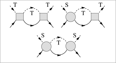
Figure 9: Right panel: leading (b,d) and next to leading (c,e) parquet diagrams determining renormalization of $J^{S}(a)$. Solid lines denote electrons in the leads. Dashed lines stand for semi-fermions representing double electron states in the dot. Left panel: irreducible diagrams contributing to RG equations. Hatched boxes and circles stand for triplet-triplet and singlet-triplet vertices respectively.

Following the ”poor man’s scaling” approach we derive the system of coupled renormalization group equations (see Fig.9) for effective couplings responsible for the finite bias $eV$ transport through DQD. As a result, the differential conductance $G(eV,T)/G_{0}\sim|J^{ST}_{LR}|^{2}$ is shown to be the universal function of two parameters $T/T_{K}$ and $eV/T_{K}$, $G_{0}=e^{2}/\pi\hbar$:

$$G/G_{0}\sim\ln^{-2}\left(\max[(eV-\delta),T]/T_{K}\right)$$ (116)

where $T_{K}$ is a non-equilibrium Kondo temperature [23]. Thus, the tunneling through singlet DQDs with the singlet/triplet splitting $\delta=E_{T}-E_{S}\gg T_{K}$ exhibits a peak in differential conductance at $eV\approx\delta$ instead of the usual zero bias Kondo anomaly which arises in the opposite limit, $\delta<T_{K}$. Therefore, in this case the Kondo effect in DQD is induced by a strong external bias. The scaling equations can also be derived in Schwinger-Keldysh formalism (see [12] and also [19]) by applying the ”poor man’s scaling” approach directly to the dot conductance. Thus, applying the semi-fermionic representation to the local (zero-dimensional) problem with dynamical symmetry [48] we developed regular perturbation theory approach and obtained the scaling equations.

3.2 From double quantum dot to spin chains and ladders

In this Section we show the application of semi-fermionic representation to 1D systems (spin chains and ladders). The semi-fermions give a powerful tool for fermionization of the spin system which can be bosonized as a next step in 1D. The bosonization procedure performed by means of Hubbard-Stratonovich transformation [52, 53, 54] is known in the literature on Tomonaga-Luttinger model as ”functional bosonization” (see also [55, 56]). It is known to be asymptotically exact in the long-wave limit. The semi-fermionic representation allows us to apply the functional bosonization methods to 1D spin systems [57]. Let us consider, as an example Spin Ladder (SL) and Spin Rotator Chain (SRC) models, Fig.10 [58]. Generic Hamiltonian for spin systems under consideration is the Heisenberg-type spin 1/2 ladder Hamiltonian

$$H^{(SL)}=J_{t}\sum_{\langle i1,i2\rangle}{\bf s}_{i1}\cdot{\bf s}_{i2}+J_{l}\sum_{\alpha}\sum_{\langle i\alpha,j\alpha\rangle}{\bf s}_{i\alpha}\cdot{\bf s}_{j\alpha}$$ (117)

Here index $\alpha=1,2$ enumerates the legs of the ladder, and the sites $\langle i1,i2\rangle$ belong to the same rung (Fig.10a). A chain of dimers of localized spins illustrated by Fig. 10b is described by the simplified version of this Hamiltonian

$$H^{SRC}=J_{t}\sum_{\langle i1,i2\rangle}{\bf s}_{i1}\cdot{\bf s}_{i2}+J_{l}\sum_{\langle ij\rangle}{\bf s}_{i1}\cdot{\bf s}_{j1}$$ (118)

The geometry of alternate rungs is chosen in a system (Fig.10b) to avoid exchange interaction between spins ${\bf s}_{i2}$ and ${\bf s}_{j2}$. The transverse coupling may emerge either from direct exchange (in case of localized spins) or from indirect Anderson-type exchange induced by tunneling (similarly to the case of quantum dots). In the latter case the sign of $J_{t}$ is antiferromagnetic, in the former case it may be ferromagnetic as well. The same is valid for $J_{l}$.

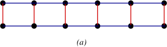
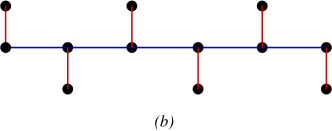
Figure 10: Spin Ladder (a) and Spin Rotator Chain (b)

As it is shown in [27, 58, 59], $SO(4)$ is an intrinsic property of S=1/2 spin ladders and decorated spin chains. To describe the elementary excitations in SRC we use the semi-fermionic representation for $SO(4)$ group (see Section I). Then the single-site Hamiltonian may be represented in a form

$$H_{i}=-E_{ST}f_{is}^{\dagger}f_{is}+h(f^{\dagger}_{i1}f_{i1}-f^{\dagger}_{i\bar{1}}f_{i\bar{1}})$$ (119)

where $h$ is uniform magnetic field applied in $z$ direction and $E_{ST}$ is a singlet/triplet splitting. Let us consider the XXZ-SRC model [27]. The Hamiltonian of this model is written in terms of the generators of $SO(4)$ group (see Appendix B) as follows

$$H=\frac{1}{4}J_{l}\sum_{\langle ij\rangle}\left(S^{+}_{i}S^{-}_{j}+S^{+}_{i}R^{-}_{j}+S^{-}_{i}R^{+}_{j}+\Delta[S^{z}_{i}S^{z}_{j}+2S^{z}_{i}R^{z}_{j}]\right).$$ (120)

The S-S part of this Hamiltonian describe the $S=1$ chain, with the Haldane gap in the excitation spectrum (see, e.g.,[60, 59]). The question is, how do the S-R interaction modifies the gap. We consider the case of FM dimers, when the triplet is the ground state. In this case one has one more gap mode, where the gap equals $J_{t}$. This mode is coupled to Haldane branch only via S-R exchange terms in (120). The spin liquid fermionization approach adopted here is a convenient tool for description of Haldane spectrum. Unlike the $S=1/2$ model, where the spin-liquid state is easily described by globally $U(1)$ invariant modes $T_{ij}T_{ji}=\sum_{\sigma}|f^{\dagger}_{i\sigma}f_{j\sigma}|^{2},$ in case of $S=1$, one deals with variables which effectively break this symmetry. One can rewrite the effective Hamiltonian of SRC model with $\Delta=0$ in a form

$$H=\frac{1}{4}J_{l}\sum_{ij}\left(f^{\dagger}_{i1}f_{j1}+f^{\dagger}_{i\bar{1}}f_{j\bar{1}}\right)\bar{B}_{j}^{0S}B_{i}^{0S}+f^{\dagger}_{i\bar{1}}f^{\dagger}_{j1}C_{j}^{0S}B_{i}^{0S}+\bar{B}_{i}^{0S}\bar{C}_{j}^{0S}f_{j1}f_{i\bar{1}},$$ (121)

where $B_{j}^{0S}=f_{0j}+f_{Sj}$ , $C_{j}^{0S}=f_{0j}-f_{Sj}$. The terms in the first line of Eq. (121) describe coherent propagation of spin fermions accompanied by a back-flow on neutral fermions, whereas the terms in the second line are ”anomalous” (they do not conserve spin fermion number). For example the propagator $\langle S^{+}_{i}S^{-}_{j}\rangle$ contains anomalous components $f^{\dagger}_{i1}f^{\dagger}_{j\bar{1}}f_{j0}f_{i0}\to F^{*}_{ij,1\bar{1}}F_{ji,00}$ along with normal ones $f^{\dagger}_{i1}f_{j1}f^{\dagger}_{j0}f_{i0}.$ Here $F_{ij,\Lambda\Lambda^{\prime}}=f_{j\Lambda}f_{i\Lambda^{\prime}}$. The first term in (121) describes the kinetic energy spinon excitations, and two last anomalous term breaking U(1) symmetry are responsible for the Haldane gap.

Figure 11: Lowest order contributions to anomalous propagator.

To reveal the contribution of dynamical symmetry on the Haldane gap, one have to note that these terms enter both in counterflow in the first term and in gauge symmetry breaking terms in the second line. In spin 1 ladder the counterflow term $\sim f^{\dagger}_{i0}f_{j0}$ predetermines the width of spinon band described by the first line of Eq. (121). Apparently, the one more channel (tripet/singlet transitions in $B^{0S}$) enhances this effect, because in this case the local constraint imposes more restrictions of phase fluctuations. The gap itself is due to anomalous correlations described by the second line of Eq. (121). Here the appearance of second channel of spinless excitations results in formation of even and odd operators $B_{j}^{0S}$ and $C_{j}^{0S}$. The Haldane gap closes when the $|0\rangle$ and $|S\rangle$ states are degenerate (the odd operator $C_{j}^{0S}$ nullifies the anomalous terms responsible for its formation). This means that appearance of $0S$ channel favors closing of the Haldane gap. In a strong coupling case of $J_{t}\gg J_{l}$ both above trends may be considered at least in the lowest order of a perturbation theory. In case of spin ladders [61, 62] the 1-st and 2-nd-order in $g=J_{l}/J_{t}$ anomalous diagrams are represented in Fig.11.

4 Epilogue and perspectives

In this paper, we demonstrated several examples of the applications of semi-fermionic representation to various problems of condensed matter physics. The list of these applications is not exhaustive. We did not discuss, e.g., the interesting development of SF approach for 2D Ising model in transverse magnetic field, functional bosonization approach based on semi-fermionic representation applied to $S=1/2$ chains, application of SF formalism to mesoscopic physics [24] etc. Nevertheless, we would like to point out some problems of strongly correlated physics where the application of SF representation might be a promising alternative to existing field-theoretical methods.

Heavy Fermions

• Crossover from localized to itinerant magnetism in Kondo lattices

• Quantum critical phenomena associated with competition between local and nonlocal correlations

• Nonequilibrium spin liquids

• Effects of spin impurities and defects in spin liquids

• Crystalline Electric Field excitations in spin liquids

• Dynamic theory of screening effects in Kondo spin glasses.

Mesoscopic systems

• Nonequilibrium Kondo effect in Quantum Dots

• Two-channel Kondo in complex multiple dots

• Spin chains, rings and ladders

• Nonequilibrium spin transport in wires

Summarizing, we constructed a general concept of semi-fermionic representation for $SU(N)$ and $SO(N)$ groups. The main advantage of this representation in application to the strongly correlated systems in comparison with another methods is that the local constraint is taken into account exactly and the usual Feynman diagrammatic codex is applicable. The method proposed allows us to treat spins on the same footing as Fermi and Bose systems. The semi-fermionic approach can be helpful for the description of the quantum systems in the vicinity of a quantum phase transition point and for the nonequilibrium spin systems.

References

References

- [1] T. Holstein and H. Primakoff, Phys. Rev. B 58, 1098 (1940).
- [2] F. Dyson, Phys. Rev. 102, 1217 (1956).
- [3] S. V. Maleyev, Sov. Phys. JETP 6, 776 (1958).
- [4] J.Schwinger, in Quantum Theory of Angular Momentum, L.C.Biedenharn and H. van Dam, Eds., Academic Press, New York, 1965, pp. 229-279.
- [5] A. A. Abrikosov, Physics 2, 5 (1965).
- [6] V. G. Vaks, A. I. Larkin, and S. A. Pikin, Sov. Phys. JETP 26, 188 (1968).
- [7] V. G. Vaks, A. I. Larkin, and S. A. Pikin, Sov. Phys. JETP 26, 647 (1968).
- [8] J. Hubbard, Proc. R. Soc. London A 285, 542 (1965).
- [9] P. Coleman, C. Pepin, and A. M. Tsvelik, Phys. Rev. B 62, 3852 (2000).
- [10] A.M.Tsvelik, Quantum field theory in condensed matter physics. Cambridge (1995)
- [11] V. N. Popov and S. A. Fedotov, Zh. Eksp. Teor. Fiz. 94, 183 (1988), [Sov. Phys. JETP 67, 535 (1988)].
- [12] M. N. Kiselev and R. Oppermann, Phys.Rev.Lett 85, 5631 (2000).
- [13] O. Veits, R. Oppermann, M. Binderberger, and J. Stein, J. Phys. I France 4, 493 (1994).
- [14] J. Stein and R. Oppermann, Z. Phys. B 83, 333 (1991).
- [15] C. Gros and M. D. Johnson, Physica B 165-166, 985 (1990).
- [16] M. N. Kiselev and R. Oppermann, JETP Lett. 71, 250 (2000).
- [17] F. Bouis and M. N. Kiselev, Physica B 259-261, 195 (1999).
- [18] S.Azakov, M.Dilaver, A.M.Oztas. Int. Journal of Modern Phys. B 14, 13 (2000).
- [19] M.N.Kiselev, H.Feldmann and R.Oppermann, Eur.Phys. J B 22, 53 (2001)
- [20] M.N.Kiselev, K.Kikoin and R.Oppermann, Phys. Rev. B 65, 184410 (2002)
- [21] R.Dillenschneider and J.Richert, cond-mat/0510434
- [22] R.Dillenschneider and J.Richert, cond-mat/0510832
- [23] M.N.Kiselev, K.Kikoin and L.W.Molenkamp, Phys. Rev. B 68, 155323 (2003).
- [24] P.Coleman and W.Mao, J. Phys.: Condens. Matter 16 L263-L269, (2004)
- [25] E. Cartan, Leçons sur la theorie des spineurs (Hermann, Paris, 1938).
- [26] N. Read and S. Sachdev, Nuc. Phys. B 316, 609 (1989).
- [27] M.N.Kiselev, D.N.Aristov, and K.Kikoin, Phys. Rev. B 71, 092404 (2005)
- [28] L.V.Keldysh. Sov. Phys. JETP 20, 1018 (1965)
- [29] J.Schwinger. J.Math.Phys. 2, 407 (1961)
- [30] V. S. Babichenko and A. N. Kozlov. Sol. St. Comm. 59, 39 (1986).
- [31] I.V.Kolokolov, Phys. Lett. 114A, 99 (1986)
- [32] I.V.Kolokolov, Sov. Phys. JETP 64, 1373 (1986)
- [33] L.B.Ioffe, A.I.Larkin. Phys.Rev. B 39, 8988 (1989).
- [34] P.A.Lee, N.Nagaosa. ibid, B 46, 5621 (1992).
- [35] A. J. Leggett, S. Chakravarty, A. T. Dorsey, M. P. A. Fisher, A. Garg, and W. Zwerger, Rev.Mod.Phys. 59, 1 (1987).
- [36] T.Brandes, Phys. Rep. 408, 315 (2005).
- [37] J.Stein and R.Oppermann, Phys.Rev. B 46, 8409 (1992)
- [38] P.Coleman, Lectures on the Physics of Highly Correlated Electron Systems VI, Editor F. Mancini, American Institute of Physics, New York (2002), p 79 - 160.
- [39] A.Tsvelik and P.B.Wiegmann, Adv.Phys. 32, 453 (1983).
- [40] N. Read and D. M. Newns, J. Phys. C 16, 3273 (1983).
- [41] K.Binder and A.P.Young, Rev. Mod. Phys. 58, 801 (1986)
- [42] D.Sherington and S.Kirkpatrick, Phys.Rev.Lett. 35, 1972 (1975)
- [43] R.Oppermann and A.Müller-Groeling, Phys. Lett. A168, 75 (1992)
- [44] R.Oppermann and A.Müller-Groeling, Nucl.Phys. B401, 507 (1993)
- [45] G.Parisi, J.Phys. A13, L115 (1980), ibid, 1101 (1980), ibid, 1887 (1980)
- [46] I.Aleiner, P.Brouwer, and L.Glazman, Phys. Rep. 358, 309 (2002).
- [47] K.Kikoin and Y.Avishai, Phys.Rev. B65, 115329 (2002).
- [48] K.A.Kikoin, Y. Avishai, and M.N.Kiselev, Dynamical symmetries in Nanophysics. pp.1-60, (NOVA Science Publisher, New York USA, in press, 2006) cond-mat/0407063
- [49] K.Kikoin and Y.Avishai, Phys.Rev.Lett. 86, 2090 (2001).
- [50] T.Kuzmenko, K.Kikoin and Y.Avishai, Phys.Rev. B 69, 195109 (2004)
- [51] L.W.Molenkamp et al., Phys. Rev. Lett. 75, 4282 (1995)
- [52] I.V.Yurkevich, Bosonisation as a Hubbard-Stratonovich Transformation In Strongly Correlated Fermions and Bosons in Low-Dimensional Disordered Systems, Edited by I.V. Lerner et al Kluwer/ Plenum, NY,P. 69 (2002)
- [53] M.Fowler, J.Phys.C: Solid St. Phys., 13, 1459 (1980)
- [54] H.C.Fogerby. J.Phys.C:Solid State Phys. 9, 3757 (1976)
- [55] A.Grishin, I.V.Yurkevich and I.V.Lerner, Phys. Rev. B 69, 165108 (2004)
- [56] I.V.Lerner and I.V.Yurkevich, cond-mat/0508223
- [57] M.N.Kiselev and D.N.Arisotv (unpublished)
- [58] K.Kikoin, Y.Avishai, and M.N.Kiselev, Explicit and Hidden Symmetries in Complex Quantum Dots and Quantum Ladders, in Molecular Nanoviers and other Quantum Objects (A.S.Alexandrov et al eds.), 177-189 (2004)
- [59] C.D.Batista and G.Ortiz, Phys. Rev. Lett. 85, 4755 (2001), Advances in Physics, 53, 1 (2004).
- [60] F.D.M. Haldane, Phys. Rev. Lett. 50, 1153 (1983); H.J. Schulz, Phys. Rev. B 34, 6372 (1986); V.A. Kashurnikov et al, Phys. Rev. B 59, 1162 (1999).
- [61] E. Dagotto, Rep. Progr. Phys. 62, 1525 (1999).
- [62] T. Barnes, E. Dagotto, J. Riera, and E.S. Swanson, Phys. Rev. B 47, 3196 (1993).
- [63] M.J. Englefield, Group Theory and the Coulomb Problem (Wiley, New York, 1972).
- [64] B.Wybourne, Classical Groups for Physicists, Willey, New York, 1974.
- [65] A.Perelomov, Generalized Coherent States and Their Applications, Springer-Verlag, Berlin, 1986.
- [66] Chou-Cheng Zhang, Science 275, 1089 (1997).