Hidden Symmetries of Electronic Transport in a Disordered One-Dimensional Lattice

Abstract

Correlated, or extended, impurities play an important role in the transport properties of dirty metals. Here, we examine, in the framework of a tight-binding lattice, the transmission of a single electron through an array of correlated impurities. In particular we show that particles transmit through an impurity array in identical fashion, regardless of the direction of transversal. The demonstration of this fact is straightforward in the continuum limit, but requires a detailed proof for the discrete lattice. We also briefly demonstrate and discuss the time evolution of these scattering states, to delineate regions (in time and space) where the aforementioned symmetry is violated.

I introduction

In a one-dimensional lattice, correlated impurities or defects may give rise to extended electronic states for particular energy levels.dunlap ; wu1 ; wu Various disordered systems with correlation have been investigated, such as the random dimer,dunlap ; wu the random trimer,giri non-symmetric dimers,lavarda the random trimer-dimer,farchioni the Thue-Morse lattice,chakrabarti and the random polymer chain.liu A built-in internal structure of the impurity configuration is important dunlap ; wu even if an internal symmetry is not necessary.lavarda In the context of electronic transport, the transmission resonance for a certain energy value implies the disordered system behaves like an ordered lattice for the corresponding electronic state, which is extended throughout the entire lattice. In this respect, it is possible to understand the increase in the conductivity for a conducting polymerwu1 .

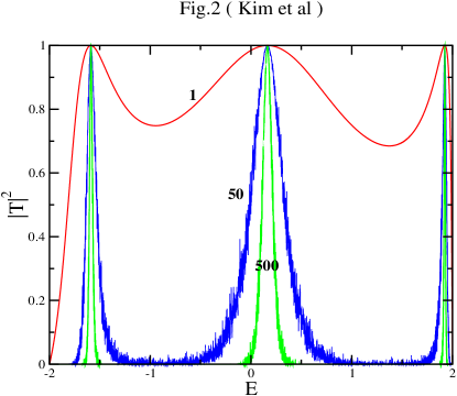
Figure 1: (Color online) Transmission probability as a function of $E$ for randomly distributed $50$ impurity dimers (blue) and $500$ dimers (green) in comparison with a single dimer (red). The inner spacing of a pair $n_{d}=3$ and the potential $V=1/2$ while the critical value $V_{0}=2/3$. The transmission probability is calculated as an ensemble average over $50$ impurity configurations.

One may, in fact, envision many other impurity configurations that give rise to extended states for various energy values. For example, let us consider a pair of impurities with a potential $V$ with respect to the lattice potential (taken to be zero). We assume that the spacing between the two impurities is always $n_{d}a$, where $a$ is the lattice constant and $n_{d}$ is a positive integer. This is then a ‘dimer’, whose length can be any value. If we adopt a tight-binding model, so that energies are given by $E=-2t_{0}\cos(ka)$, where $t_{0}$ is the nearest-neighbor hopping amplitude, then one can obtain the transmission probability $|T|^{2}$ for this state. It is

$$|T|^{2}=\frac{\sin^{2}(k)}{\sin^{2}(k)+V^{2}\left[\cos(kn_{d})+\frac{V}{2}\frac{\sin(kn_{d})}{\sin(k)}\right]^{2}}\;.$$ (1)

where $t_{0}$ and $a$ have been set to unity for simplicity. Inspection of Eq. (1) reveals a critical strength of the impurity potential $V_{c}/t_{0}=\pm 2/n_{d}$ for repulsive and attractive interactions, respectively, which determines how many states are extended, i.e. have unit transmission. A graphical construction readily shows that, for $V>2/n_{d}$, there are $n_{d}-1$ extended states while for $V\leq 2/n_{d}$, there are $n_{d}$ extended states. As in the nearest-neighbor dimer case, consideration of one ‘dimer’ helps us to understand electronic transport in a lattice with many ‘dimers’, following the analysis of Ref.dunlap . In Fig. 1, we show $|T|^{2}$ as a function of $E$ for randomly distributed $50$ impurity dimers (blue) and $500$ dimers (green) in comparison with a single dimer (red). The inner spacing of a pair $n_{d}=3$ and the potential $V=1/2$. Note that in this instance $V<V_{c}=2/3$. The transmission probability is calculated to be an ensemble average over $50$ impurity configurations. Remarkably, the transmission remains unity at the three energies for which a single ‘dimer’ has unit transmission, and the ’width’ of the resonance narrows as the number of impurities increases.

This specific example is given by way of introduction to more general considerations of impurity potentials on a lattice. In this paper we will show there exist hidden symmetries underlying the physics of electronic transport in a one-dimensional lattice with an arbitrary impurity configuration, using the transfer matrix formalism. We will also demonstrate the time evolution of a wave packet by direct diagonalization of the Hamiltonian since the transfer matrix formalism does not produce the dynamics of a wave function. While the dynamics can be insightful, we are also hopeful that present-day technology can spatially and temporally resolve some of the interesting dynamics that result from our (and future) work.

Perhaps the most general correlated impurity configuration is the following. Suppose there are $N$ impurities A₁A${}_{2}\cdots$A_N embedded at the sites $1$ through $N$ in a host lattice. The corresponding impurity potentials are given by $(U_{1},\;U_{2},\;\cdots,\;U_{N})$, where $U_{i}\;(i=1,\cdots,N)$ can be positive, zero, or negative. Our main result is that the transmission amplitude $T$ for this impurity configuration is identical to $T$ for its reverse configuration; namely, $T(U_{1},\;U_{2},\;\cdots,\;U_{N})=T(U_{N},\;U_{N-1},\;\cdots,\;U_{1})$. Given this then obviously the equality holds for the transmission $|T|^{2}$ and reflection $|R|^{2}$ probabilities. In other words, $|T|^{2}$ and $|R|^{2}$ are independent of the direction of the incoming wave. This symmetry is striking because the impurity configuration is assumed arbitrary without possessing any parity. For example, it has been shown that the chains of ABBABAAB$\cdots$ and BAABABBA$\cdots$ contribute identically for electronic transportchakrabarti . This is a simple example of the general symmetry we describe. Note that an exchange of any two impurity potentials does not show this symmetry; for example, $T(U_{1},\;U_{2},\;U_{3},\;U_{4})\neq T(U_{2},\;U_{1},\;U_{3},\;U_{4})$ wkb .

We should emphasize now that this symmetry does not hold in the impurity region (as perhaps one would expect), but this can only be determined by solving the time-dependent Schrödinger equation (see below). We also explain another symmetry associated with a particular momentum $k=\pi/(2a)$, where $a$ is the lattice constant: $|T(U_{1},\;U_{2},\;\cdots,\;U_{N})|^{2}=|T(-U_{1},\;-U_{2},\;\cdots,\;-U_{N})|^{2}$. This equality indicates a potential barrier or well produces identical transmission and reflection probabilities for the electronic state with $k=\pi/(2a)$. This is unrelated to the other remarkable feature of wave packets on a one-dimensional lattice with nearest-neighbor hopping and $k=\pi/(2a)$: they do not diffuse as a function of time, because they lack group velocity dispersion. Indeed, one can show that no matter what the range of the hopping is, there will be a wave vector for which the wave packet retains its initial width.

II formalism

We start with a tight-binding Hamiltonian for a one-dimensional lattice with $N$ impurities:

$$H=-t_{0}\sum_{i}\left[c^{+}_{i}c_{i+1}+c^{+}_{i+1}c_{i}\right]+\sum_{i\in{\cal I}}U_{i}c^{+}_{i}c_{i}$$ (2)

where the hopping amplitude $t_{0}$ will be set to be unity, $c^{+}_{i}$ creates an electron at a site $i$, and ${\cal I}$ represents an impurity configuration. The Schrödinger equation is $H|\psi\rangle=E|\psi\rangle$ with $|\psi\rangle=\sum_{j}\psi_{j}c^{+}_{j}|0\rangle$; this becomes

$$-\left[\psi_{j+1}+\psi_{j-1}\right]+U_{j}\psi_{j}=E\psi{j}$$ (3)

where $\psi_{j}$ is an amplitude to find an electron at site $j$. In order to use the transfer matrix formalism we write Eq. (3) in a matrix form as follows:

$$\left(\begin{array}[]{c}\psi_{j+1}\\ \psi_{j}\end{array}\right)=\left(\begin{array}[]{cc}U_{i}-E&-1\\ 1&0\end{array}\right)\left(\begin{array}[]{c}\psi_{j}\\ \psi_{j-1}\end{array}\right)\equiv M_{j}\left(\begin{array}[]{c}\psi_{j}\\ \psi_{j-1}\end{array}\right)\;.$$ (4)

Note that $M_{i}$ is a unimodular matrix, i.e. $\det(M_{i})=1$. The wave functions $\psi_{L}$ (for $i<1$) and $\psi_{R}$ (for $i>N$) are $\psi_{L}=e^{ikx_{i}}+R\;e^{-ikx_{i}}$ and $\psi_{R}=T\;e^{ikx_{i}}$, where $x_{i}=a\cdot i$. Using the transfer matrix formalism, one can express the coefficients $R$ and $T$ in terms of $k$, $U_{i}$, and $E$ as follows:

$$\left(\begin{array}[]{c}T\\ iT\end{array}\right)=P\left(\begin{array}[]{c}1+R\\ i(1-R)\end{array}\right)\;,$$ (5)

where $P=S^{-1}MS$ with $S=\left(\begin{array}[]{cc}\cos(k)&\sin(k)\\ 1&0\end{array}\right)$, and $M=M_{N}M_{N-1}\cdots M_{1}$. It is misleading to express $M=\Pi^{N}_{i=1}M_{i}$ because $M_{i}$ and $M_{j}$ $(i\neq j)$ do not commute with each other. Solving Eq. (5), one can obtainburrow

$$T = \frac{2i}{i\left(P_{11}+P_{22}\right)+P_{12}-P_{21}}$$ (6)

$$R = \frac{P_{12}+P_{21}-i\left(P_{11}-P_{22}\right)}{i\left(P_{11}+P_{22}\right)+P_{12}-P_{21}}\;.$$ (7)

Consequently, the transmission probability $|T|^{2}=4\big{/}\left[\mbox{tr}(P{\tilde{P}})+2\right]$ and the reflection probability $|R|^{2}=\left[\mbox{tr}(P{\tilde{P}})-2\right]\big{/}\left[\mbox{tr}(P{\tilde{P}})+2\right]$, where tr$(P)$ means the trace of $P$, and ${\tilde{P}}$ is the transpose of $P$. Note that Eq. (1) is readily obtained with this formalism by using $M^{\prime}=M_{V}M^{n_{d}-1}_{0}M_{V}$, where $M_{V}=M_{1}(U_{1}=V)$ and $M_{0}=M_{1}(U_{1}=0)$, and $n_{d}$ is the inner spacing of the impurity pair.

One of the symmetries we introduced earlier is $T(U_{1},\;U_{2},\cdots,\;U_{N})=T(U_{N},\;U_{N-1},\cdots,\;U_{1})$. In order to show this equality, let us introduce $Q=S^{-1}M^{\prime}S$ where $M^{\prime}=M_{1}M_{2}\cdots M_{N}$. Notice the order of the matrix multiplication because $M_{i}$ and $M_{j}$ $(i\neq j)$ do not commute with each other. Since the desired equality implies that $T[P]=T[Q]$, we need to show $P_{11}+P_{22}=Q_{11}+Q_{22}$ and $P_{12}-P_{21}=Q_{12}-Q_{21}$. On the other hand, from the definitions of $P=S^{-1}MS$ and $Q=S^{-1}M^{\prime}S$, this equality in turn implies that $M_{11}=M^{\prime}_{11}$, $M_{22}=M^{\prime}_{22}$, and $M_{12}-M_{21}=M^{\prime}_{12}-M^{\prime}_{21}$. Note, however, that in general $M\neq M^{\prime}$, as we will show later.

For simplicity, we define ${\cal U}_{i}=U_{i}-E$. We also introduce $2\times 2$ matrices $\alpha$ and $\beta$ such as $\alpha=\left(\begin{array}[]{cc}1&0\\ 0&0\end{array}\right)$ and $\beta=\left(\begin{array}[]{cc}0&-1\\ 1&0\end{array}\right)$ to have $M_{i}={\cal U}_{i}\alpha+\beta$. Note that $\alpha^{2}=\alpha$, $\beta^{2}=-1$, $\alpha\beta+\beta\alpha=\beta$, and $\alpha\beta\alpha=0$. Since $M=M_{N}M_{N-1}\cdots M_{1}$, we obtain

$$M = ({\cal U}_{N}\alpha+\beta)({\cal U}_{N-1}\alpha+\beta)\cdots({\cal U}_{1}\alpha+\beta)$$ (8)

$$= \beta^{N}+\sum^{N}_{n}\sum^{N}_{\{j_{n}\}}({\cal U}_{j_{1}}{\cal U}_{j_{2}}\cdots{\cal U}_{j_{n}})\beta^{N-j_{n}}\alpha\beta^{j_{n}-j_{n-1}-1}\alpha\cdots\alpha\beta^{j_{2}-j_{1}-1}\alpha\beta^{j_{1}-1}\;,$$

where $\{j_{n}\}$ means $j_{1},j_{2},\cdots,j_{n}=1,2,,\cdots,N$ with $j_{1}<j_{2}<\cdots<j_{n}$. Since $\alpha\beta\alpha=0$ and $\beta^{2}=-1$, non-vanishing terms should have $j_{l}-j_{l-1}-1=\mbox{even}$, where $l=2,3,\cdots n$ for a given $n$. Therefore, we obtain

$$M=\beta^{N}+\sum^{N}_{n}\sum^{N}_{\{\{j_{n}\}\}}({\cal U}_{j_{1}}{\cal U}_{j_{2}}\cdots{\cal U}_{j_{n}})(-1)^{\frac{1}{2}(j_{n}-j_{1}-n+1)}\beta^{N-j_{n}}\alpha\beta^{j_{1}-1}\;,$$ (9)

where $\{\{j_{n}\}\}$ means $\{j_{n}\}$ with $j_{l}-j_{l-1}-1=\mbox{even}$. Since $\alpha=\left(\begin{array}[]{cc}1&0\\ 0&0\end{array}\right)$, $\alpha\beta=\left(\begin{array}[]{cc}0&-1\\ 0&0\end{array}\right)$, $\beta\alpha=\left(\begin{array}[]{cc}0&0\\ 1&0\end{array}\right)$, and $\beta\alpha\beta=\left(\begin{array}[]{cc}0&0\\ 0&-1\end{array}\right)$, we use these as the basis matrices to expand $M$:

$$M=c_{1}\alpha+c_{2}\alpha\beta+c_{3}\beta\alpha+c_{4}\beta\alpha\beta=\left(\begin{array}[]{cc}c_{1}&-c_{2}\\ c_{3}&-c_{4}\end{array}\right)\;.$$ (10)

As we mentioned, the equality of the transmission amplitude, $T[P]=T[Q]$, is associated with some particular relations among the components of the two matrices $M=M_{1}M_{2}\cdots M_{N}$ and $M^{\prime}=M_{N}M_{N-1}\cdots M_{1}$. Following the same way as for $M$, we expand $M^{\prime}$ in terms of ${\cal U}_{i}\;(i=1,2,\cdots,N)$, $\alpha$, and $\beta$ to obtain

$$M^{\prime} = ({\cal U}_{1}\alpha+\beta)({\cal U}_{2}\alpha+\beta)\cdots({\cal U}_{N}\alpha+\beta)$$ (11)

$$= \beta^{N}+\sum^{N}_{n}\sum^{N}_{\{j_{n}\}}({\cal U}_{j_{1}}{\cal U}_{j_{2}}\cdots{\cal U}_{j_{n}})\beta^{j_{1}-1}\alpha\beta^{j_{2}-j_{1}-1}\alpha\cdots\alpha\beta^{j_{n}-j_{n-1}-1}\alpha\beta^{N-j_{n}}\;.$$

It is also true for $M^{\prime}$ that non-vanishing terms have $j_{l}-j_{l-1}-1=\mbox{even}$ because $\alpha\beta\alpha=0$. Therefore,

$$M^{\prime}=\beta^{N}+\sum^{N}_{n}\sum^{N}_{\{\{j_{n}\}\}}({\cal U}_{j_{1}}{\cal U}_{j_{2}}\cdots{\cal U}_{j_{n}})(-1)^{\frac{1}{2}(j_{n}-j_{1}-n+1)}\beta^{j_{1}-1}\alpha\beta^{N-j_{n}}\;.$$ (12)

Expanding $M^{\prime}$, again, in terms of the basis matrices, we know

$$M^{\prime}=c^{\prime}_{1}\alpha+c^{\prime}_{2}\alpha\beta+c^{\prime}_{3}\beta\alpha+c^{\prime}_{4}\beta\alpha\beta=\left(\begin{array}[]{cc}c^{\prime}_{1}&-c^{\prime}_{2}\\ c^{\prime}_{3}&-c^{\prime}_{4}\end{array}\right)\;.$$ (13)

Comparing Eqs. (10) and (13), the equalities $M_{11}=M^{\prime}_{11}$, $M_{22}=M^{\prime}_{22}$, and $M_{12}-M_{21}=M^{\prime}_{12}-M^{\prime}_{21}$ are equivalent to the equalities $c_{1}=c^{\prime}_{1}$, $c_{4}=c^{\prime}_{4}$, and $c_{2}+c_{3}=c^{\prime}_{2}+c^{\prime}_{3}$. Since $\beta^{N}$ does not depend on ${\cal U}_{i}$ and $\beta^{N}=(-1)^{N/2}$ or $(-1)^{(N-1)/2}\beta$ for even (or odd) $N$, we can ignore $\beta^{N}$ for the purpose of showing these equalities, or, alternatively, we can redefine $M$ as $M-\beta^{N}$ and $M^{\prime}$ and $M^{\prime}-\beta^{N}$. To obtain i) $c_{1}$ of $M$, we should have $j_{1}-1=$ even and $N-j_{n}=$ even. Similarly, ii) for $c_{2}$, $j_{1}-1=$ odd and $N-j_{n}=$ even, iii) for $c_{3}$, $j_{1}-1=$ even and $N-j_{n}=$ odd, and iv) for $c_{4}$, $j_{1}-1=$ odd and $N-j_{n}=$ odd. In terms of ${\cal U}_{i}$, we obtain

$$c_{1} = \sum^{N}_{n}\sum^{N}_{\{\{j_{n}\}\}_{1}}({\cal U}_{j_{1}}{\cal U}_{j_{2}}\cdots{\cal U}_{j_{n}})(-1)^{\frac{1}{2}(N-n)}$$

$$c_{2} = \sum^{N}_{n}\sum^{N}_{\{\{j_{n}\}\}_{2}}({\cal U}_{j_{1}}{\cal U}_{j_{2}}\cdots{\cal U}_{j_{n}})(-1)^{\frac{1}{2}(N-n-1)}$$

$$c_{3} = \sum^{N}_{n}\sum^{N}_{\{\{j_{n}\}\}_{3}}({\cal U}_{j_{1}}{\cal U}_{j_{2}}\cdots{\cal U}_{j_{n}})(-1)^{\frac{1}{2}(N-n-1)}$$

$$c_{4} = \sum^{N}_{n}\sum^{N}_{\{\{j_{n}\}\}_{4}}({\cal U}_{j_{1}}{\cal U}_{j_{2}}\cdots{\cal U}_{j_{n}})(-1)^{\frac{1}{2}(N-n-2)}$$

where $\{\{j_{n}\}\}_{1}$ means $\{\{j_{n}\}\}$ with $(j_{1}-1,N-j_{n})=$ (even, even). Similarly, $\{\{j_{n}\}\}_{2}=$ $\{\{j_{n}\}\}$ with (odd, even), $\{\{j_{n}\}\}_{3}=$ $\{\{j_{n}\}\}$ with (even, odd), and $\{\{j_{n}\}\}_{4}=$ $\{\{j_{n}\}\}$ with (odd, odd).

For $c^{\prime}_{1}$, $c^{\prime}_{2}$, $c^{\prime}_{3}$, and $c^{\prime}_{4}$ of Eq. (13), we should have $(j_{1}-1,N-j_{n})=$ (even, even), (even, odd), (odd, even), and (odd, odd), respectively. Note that we need (even, odd) for $c^{\prime}_{2}$ while (odd, even) for $c_{2}$. On the other hand, we need (odd, even) for $c^{\prime}_{3}$ while (even, odd) for $c_{3}$. Therefore, we obtain

$$c^{\prime}_{1} = \sum^{N}_{n}\sum^{N}_{\{\{j_{n}\}\}_{1}}({\cal U}_{j_{1}}{\cal U}_{j_{2}}\cdots{\cal U}_{j_{n}})(-1)^{\frac{1}{2}(N-n)}$$

$$c^{\prime}_{2} = \sum^{N}_{n}\sum^{N}_{\{\{j_{n}\}\}_{3}}({\cal U}_{j_{1}}{\cal U}_{j_{2}}\cdots{\cal U}_{j_{n}})(-1)^{\frac{1}{2}(N-n-1)}$$

$$c^{\prime}_{3} = \sum^{N}_{n}\sum^{N}_{\{\{j_{n}\}\}_{2}}({\cal U}_{j_{1}}{\cal U}_{j_{2}}\cdots{\cal U}_{j_{n}})(-1)^{\frac{1}{2}(N-n-1)}$$

$$c^{\prime}_{4} = \sum^{N}_{n}\sum^{N}_{\{\{j_{n}\}\}_{4}}({\cal U}_{j_{1}}{\cal U}_{j_{2}}\cdots{\cal U}_{j_{n}})(-1)^{\frac{1}{2}(N-n-2)}$$

Consequently, we have $c_{1}=c^{\prime}_{1}$, $c_{4}=c^{\prime}_{4}$, and $c_{2}+c_{3}=c^{\prime}_{2}+c^{\prime}_{3}$; in other words, $T[P]=T[Q]$, or equivalently, $T(U_{1},\;U_{2},\;\cdots,\;U_{N})=T(U_{N},\;U_{N-1},\;\cdots,\;U_{1})$ In fact, $M_{12}=-M^{\prime}_{21}$ and $M_{21}=-M^{\prime}_{12}$. Note, however, that in general $M\neq M^{\prime}$.

One may anticipate a similar symmetry in the continuum limit.arias Consider a time-dependent Schödinger equation: $i\partial_{t}\psi(t,x)=H(x)\psi(t,x)$, where the Hamiltonian $H(x)$ includes an impurity potential $V(x)$ for $|x|\leq l$. The wave function for $|x|>l$ can be represented as $\psi(|x|>l)=\left[e^{ikx}+Re^{-ikx}\right]\Theta(-x-l)+Te^{ikx}\Theta(x-l)$, where $\Theta(x)$ is the step function. Let us introduce another time-dependent Schödinger equation: $i\partial_{t}\psi^{\prime}(t,x)=H(-x)\psi^{\prime}(t,x)$, where $\psi(|x|>l)=\left[e^{ikx}+R^{\prime}\;e^{-ikx}\right]\Theta(-x-l)+T^{\prime}\;e^{ikx}\Theta(x-l)$. Invoking both space inversion and time reversal, one can see that $\psi(t,-x)$ and $\psi^{*}(-t,-x)$ satisfy the same equation as $\psi^{\prime}(t,x)$ does. Equating $a_{1}\psi(t,-x)+a_{2}\psi^{*}(-t,-x)=\psi^{\prime}(t,x)$ for $|x|>l$ leads to $T^{\prime}=T$ and $R^{\prime}T^{*}+R^{*}T=0$. The first relation corresponds to $T[P]=T[Q]$ in a lattice. The second relation, however, does not hold in a lattice. Instead, we found in a lattice

$$\frac{T^{*}[P]\left(R[Q]-R[P]\right)}{T[P]\left(R^{*}[Q]-R^{*}[P]\right)}=e^{2ik}\;.$$ (14)

Nevertheless, we can still define $R[Q]=e^{i\delta}R[P]$. The phase $\delta$ is determined by $e^{i\delta}=-e^{2ik}\;R^{*}T/(RT^{*})$ in a lattice while $e^{i\delta}=-R^{*}T/(RT^{*})$ in the continuum limit.

We also found another symmetry associated with electronic transport in a one-dimensional lattice; in this case there is no applicability in the continuum limit. Suppose $k=\pi/2$; then $S=\left(\begin{array}[]{cc}0&1\\ 1&0\end{array}\right)$, and $S={\tilde{S}}=S^{-1}$. Note that for a symmetric $(2\times 2)$ matrix $X$ such that $X={\tilde{X}}$, $M_{i}$ satisfies $M_{i}X{\tilde{M}}_{i}={\tilde{M}}_{i}XM_{i}$ with ${\cal U}_{i}\rightarrow-{\cal U}_{i}$. Now let us consider $\mbox{tr}(P{\tilde{P}})$:

$$\mbox{tr}\left(P{\tilde{P}}\right) = \mbox{tr}\left(M_{N}\cdots M_{1}{\tilde{M}}_{1}\cdots{\tilde{M}}_{N}\right)$$ (15)

$$= \mbox{tr}\left({\tilde{M}}_{N}\cdots{\tilde{M}}_{1}M_{1}\cdots M_{N}\right)_{{\cal U}\rightarrow-{\cal U}}$$

$$= \mbox{tr}\left({\tilde{Q}}Q\right)_{-{\cal U}}=\mbox{tr}\left(Q{\tilde{Q}}\right)_{-{\cal U}}$$

This symmetry indicates that for $k=\pi/2$, $|T|^{2}$ and $|R|^{2}$ depend only on $|{\cal U}_{i}|$. If $E=-2\cos(k)$, then ${\cal U}_{i}=U_{i}$. In this instance, $|T(U_{1},\cdots,U_{N})|^{2}=|T(-U_{N},\cdots,-U_{1})|^{2}$. Since $|T(U_{1},\cdots,U_{N})|^{2}=|T(U_{N},\cdots,U_{1})|^{2}$ from a general derivation, $|T(U_{1},\cdots,U_{N})|^{2}=|T(-U_{1},\cdots,-U_{N})|^{2}$. Consequently, a potential barrier and a potential well give identical transmission and reflection probabilities for $k=\pi/2$ and $E=-2\cos(k)$.

III time evolution of a wave packet

So far we have been using the transfer matrix formalism. Since, however, the transfer matrix formalism is based on the time-independent Schrödinger equation, we cannot see the time evolution of a wave function, which may indicate the significance of the symmetries we have shown. Let us consider a wave packet with average position $x_{0}$ and average momentum $k_{0}$ at time $t=0$: $|\Psi(0)\rangle=\sum_{i}\varphi(x_{i},0)c^{+}_{i}|0\rangle$, where

$$\varphi(x_{i},0)=\frac{1}{(2\pi\alpha^{2})^{1/4}}e^{ik_{0}(x_{i}-x_{0})}e^{-\frac{1}{4}(x_{i}-x_{0})^{2}/\alpha^{2}}\;.$$ (16)

We introduced the initial uncertainty $\alpha$ associated with position. We wish to propagate (in real time) this wave packet towards the potentials. To do this we first diagonalize the Hamiltonian, which is an $(L\times L)$ matrix, where $L$ is the total number of lattice sites under consideration. We thus obtain the eigenstates $|n\rangle$ and the corresponding eigenvalues $\epsilon_{n}$ such that $H|n\rangle=\epsilon_{n}|n\rangle$. An eigenstate is a column vector with $L$ components which describes the probability of finding an electron at a particular site in the lattice. With eigenstates in hand, the time evolution of the wave packet is given by

$$|\Psi(t)\rangle=\sum^{L}_{n=1}|n\rangle\langle n|\Psi(0)\rangle e^{-i\epsilon_{n}t}\;.$$ (17)

As time goes on, the wave packet initially at $x_{0}$ moves to the potential region and scatters off the potential. A part of the wave packet is reflected and the other part is transmitted. Mathematically we can define the reflection and the transmission as $|R|^{2}=\sum_{left}|\varphi(x_{i},t)|^{2}$ and $|T|^{2}=\sum_{right}|\varphi(x_{i},t)|^{2}$, respectively as $t\rightarrow\infty$, where $\sum_{left(right)}$ means the summation includes only the left(right) side of the impurity region.

Figure 2: Time evolution of a wave packet in two impurity configurations [I] (red solid) and [II] (blue dashed curve). Each configuration has 5 impurities: for [I] the potential is $(-0.5,\;0,\;0.5,\;1.5,\;1)$ while for [II] its reverse holds.

Fig. 2 shows the time evolution of a wave packet impinging on 5 impurities located at sites $300$ to $304$. The parameters of the wave packet are given as follows: $x_{0}=150$, $\alpha=20$, and $k_{0}=\pi/3$. Note we choose $\alpha=20$ so that the size of the wave packet is much greater than the size of the impurity region. This means that we can consider the wave packet as a plane wave in this case. In fact, the numerical results of the transmission and reflection probabilities are in close agreement with those obtained through the transfer matrix analysis. The impurity configuration is determine by 5 impurity potentials: $(U_{1},\;U_{2},\;U_{3},\;U_{4},\;U_{5})$. For [I] (red solid), we have $(-0.5,\;0,\;0.5,\;1.5,\;1)$ while for [II] (blue dashed curve), we have the reverse order. As clearly shown in Fig. 2, the time evolution of the wave packet is different depending on the impurity configurations. In particular, the scattering completely differentiates [I] from [II], as indicated by the very differently behaved red and blue curves in the scattering region. Nonetheless the probability that emerges (either in transmission or reflection) is identical for both, in agreement with the symmetry we just proved. Note that the transmitted wave packets are identical in all other respects as well whereas the reflected wave packets have identical shape, but are phase-shifted with respect to one another. In fact, one can show that the phase shift originates from the phase $\delta$ in $R[Q]=e^{i\delta}\;R[P]$. The shift measured by the difference between the two reflected wave packets for [I] and [II] at their half width is determined by $\partial\delta(k)/\partial k\big{|}_{k_{0}}$.

IV conclusions

We have determined the transmission and reflection characteristics for various impurity configurations on a one dimensional lattice. In particular we proved that the transmission of a particle through an array of impurities is independent of the direction of travel. This theorem may help understand, among other things, weak localization, where time-reversed paths play an important role. Some important differences arise because of the lattice: first, it becomes clear that the group velocity is most important (in the continuum limit the energy is usually emphasized). Secondly, other symmetries exist on a lattice for particular wavevectors. Naturally these symmetries do not hold in the actual scattering region. While we have no specific proposals at present, we hope this work motivates experimentalists to look for these violations in the vicinity of particular impurity configurations. Further work is in progress with trimer impurity configurations, more general band structures, and higher dimensionality.

This work was supported in part by the Natural Sciences and Engineering Research Council of Canada (NSERC), by ICORE (Alberta), and by the Canadian Institute for Advanced Research (CIAR). FM is appreciative of the hospitality of the Department of Condensed Matter Physics at the University of Geneva.

References

• (1) D.H. Dunlap, H.-L. Wu, and P. Phillips, Phys. Rev. Lett. 65, 88 (1990).
• (2) H.-L. Wu, and P. Phillips, Phys. Rev. Lett. 66, 1366 (1991).
• (3) H.-L. Wu, W. Goff, and P. Phillips, Phys. Rev. B45, 1623 (1992).
• (4) D. Giri, P.K. Datta, and K. Kundu, Phys. Rev. B48, 14113 (1993).
• (5) F.C. Lavarda, M.C. dos Santos, D.S. Galvão, and B. Laks, Phys. Rev. Lett. 73, 1267 (1994).
• (6) R. Farchioni and G. Grosso, Phys. Rev. B56, 1170 (1997).
• (7) A. Chakrabarti, S.N. Karmakar, and R.K. Moitra, Phys. Rev. Lett. 74, 1403 (1995).
• (8) Y.M. Liu, R.W. Peng, X.Q. Huang, M. Wang, A, Hu, and S.S. Jian, Phys. Rev. B67, 205209 (2003)
• (9) The WKB approximation would incorrectly show this symmetry, for example, so, while the WKB approximation clearly satisfies the symmetry which we are about to prove, it is unreliable as a diagnostic tool.
• (10) B.L. Burrow and K.W. Sulton, Phys. Rev. B51, 5732 (1995).
• (11) For a graphic description, see T.A. Aris, Note on Feynman diagrams for scattering problems in one dimension (unpublished).