Simulating (electro)hydrodynamic effects in colloidal dispersions: smoothed profile method

Abstract

Previously, we have proposed a direct simulation scheme for colloidal dispersions in a Newtonian solvent [Phys.Rev.E 71,036707 (2005)]. An improved formulation called the ”Smoothed Profile (SP) method” is presented here in which simultaneous time-marching is used for the host fluid and colloids. The SP method is a direct numerical simulation of particulate flows and provides a coupling scheme between the continuum fluid dynamics and rigid-body dynamics through utilization of a smoothed profile for the colloidal particles. Moreover, the improved formulation includes an extension to incorporate multi-component fluids, allowing systems such as charged colloids in electrolyte solutions to be studied. The dynamics of the colloidal dispersions are solved with the same computational cost as required for solving non-particulate flows. Numerical results which assess the hydrodynamic interactions of colloidal dispersions are presented to validate the SP method. The SP method is not restricted to particular constitutive models of the host fluids and can hence be applied to colloidal dispersions in complex fluids.

1 Introduction

Interparticle interactions in colloidal dispersions mainly consist of thermodynamic potential interactions and hydrodynamic interactions happel83:_low_reynol ; kim91:_microh ; russel89:_colloid_disper . Whereas the former interactions occur in both static and dynamic situations, the latter occur solely in dynamic situations. Although thermodynamic interactions have been studied extensively and summarized as a concept of the effective interaction likos01:_effec , the nature of dynamic interactions is poorly understood. Since the hydrodynamic interaction is essentially a long-range, many-body effect, it is extremely difficult to study its role using analytical methods alone. Numerical simulations can aid the investigation of the fundamental role of hydrodynamic interactions in colloidal dynamics.

In recent decades, various simulations for particulate flow have been developed for most simple situations in which the host fluid is Newtonian brady88:_stokes_dynam ; malevanets99:_mesos ; tanaka00:_simul_method_colloid_suspen_hydrod_inter ; kajishima01:_turbul_struc_partic_laden_flow ; hu01:_direc_numer_simul_fluid_solid ; glowinski01:_fictit_domain_approac_direc_numer ; ladd01:_lattic_boltz ; padding04:_hydrod_brown_fluct_sedim_suspen ; cates04:_simul_boltz . However, these schemes can not necessarily be applied to problems with non-Newtonian host fluids or solvents with internal microstructures, which are practically more important cases. Hydrodynamic simulations of ions and/or charged colloids have been proposed by making use of some of the above schemes kim05:_elect ; yamaue05:_multi_phase_dynam_progr_manual ; lobaskin04:_elect ; chatterji05:_combin_lattic_boltz ; capuani04:_discr ; capuani06:_lattic_boltz . Nonetheless, the tractability and/or physical validity of their modeling remain controversial. In Ref.kim05:_elect , in solving the motion of the ionic solutes, the solvent hydrodynamic interaction was incorporated by Rotne–Pragar–Yamakawa-type mobility tensor, which accounted for a long-range part of pair interaction. This scheme misses many-body and/or near-field hydrodynamic interactions between the solutes and surfaces, which can have an effects on the behavior of ions near surface. In Ref.yamaue05:_multi_phase_dynam_progr_manual , the computational mesh was arranged to express round shape of a colloidal particle and the boundary value problem of the solvent continuum equations was solved based on the irregular mesh. For applying this scheme to many-body system, inaccessible computational resources is inevitable. In Refs.lobaskin04:_elect ; chatterji05:_combin_lattic_boltz ; capuani04:_discr ; capuani06:_lattic_boltz , they adopted the lattice Boltzmann (LB) method for explicitly solving the solvent hydrodynamics. Although the LB method has many advantages for solving large systems, compared to the standard discretization schemes, the applicability to various constitutive equations for the complex fluids other from the Newtonian fluids is unveiled. Concerning the interaction between colloidal particles and the solvent, authors in Refs lobaskin04:_elect ; chatterji05:_combin_lattic_boltz , arranged finite interaction points on the surface of the colloids on which a frictional coupling was assumed. In this coupling scheme, friction parameters and the number of the interaction points were determined phenomenologically and theoretical basis to determine the parameters in general systems was not clearly stated.

In this article, we propose a direct simulation scheme for colloidal dispersions which is applicable to most constitutive models of the host fluids. We call it the ”Smoothed Profile (SP) method” since the original sharp interface between the colloids and solvent is replaced with an effective smoothed interface with a finite thickness tanaka00:_simul_method_colloid_suspen_hydrod_inter ; nakayama05:_simul_method_resol_hydrod_inter_colloid_disper . We formulate a computational method to couple the particle dynamics and hydrodynamics of the solvent. A fixed grid is used in both the solvent and the particle domains. Introduction of a smoothed profile makes it possible to realize stable and efficient implementation of our scheme. The numerical implementation for Newtonian solvents and electrolyte solutions as specific examples of multi-component fluids is outlined. Various test cases which verify the SP method and assess the hydrodynamic interactions are presented.

2 Dynamics of a multi-component solvent and colloids

2.1 Hydrodynamics of multi-component fluids

We first give a brief description of multi-component fluid equations, looking at electrolyte solutions as a specific application. Consider $N$ (possibly ionic) solute species that satisfy the law of conservation for every concentration, $C_{\alpha}$, of the $\alpha$th species:

$$\partial_{t}C_{\alpha}+\nabla\cdot C_{\alpha}\mbox{\boldmath$v$}_{\alpha}+\nabla\cdot\mbox{\boldmath$g$}_{\alpha} =0,$$ (1)

where $\mbox{\boldmath$v$}_{\alpha}$ is the velocity of the $\alpha$th solute and $\mbox{\boldmath$g$}_{\alpha}$ is a random current. Since the inertial time scales of the solute molecules are extremely small, the velocity of the $\alpha$th solute can be decomposed into the velocity of the solvent $v$ and the diffusive current arising from the chemical potential gradient $\nabla\mu_{\alpha}$ as:

$$\mbox{\boldmath$v$}_{\alpha} =\mbox{\boldmath$v$}-\Gamma_{\alpha}\nabla\mu_{\alpha},$$ (2)

where $\Gamma_{\alpha}k_{B}T$ is the diffusivity of the $\alpha$th ion, $k_{B}$ is the Boltzmann constant and $T$ is the temperature. The random current should satisfy the following fluctuation-dissipation relation landau59:_fluid :

$$\langle g_{\alpha,i}(\mbox{\boldmath$x$},t)g_{\beta,j}(\mbox{\boldmath$x$}^{\prime},t^{\prime})\rangle =2(k_{B}T)^{2}\Gamma_{\alpha}\delta_{\alpha\beta}\delta_{ij}\delta(\mbox{\boldmath$x$}-\mbox{\boldmath$x$}^{\prime})\delta(t-t^{\prime}).$$ (3)

Here, for the sake of simplicity, we do not deal with the cross diffusion of different solutes. The conservation of momentum implies the velocity of solvent follows the Navier–Stokes equation of incompressible flow with the source term from solutes:

$$\nabla\cdot\mbox{\boldmath$v$} =0,$$ (4)

$$\rho\left(\partial_{t}+\mbox{\boldmath$v$}\cdot\nabla\right)\mbox{\boldmath$v$} =-\nabla p+\eta\nabla^{2}\mbox{\boldmath$v$}-\sum_{\alpha}C_{\alpha}\nabla\mu_{\alpha}+\nabla\cdot\mbox{\boldmath$s$},$$ (5)

where $\rho$ is the total mass density of the fluid, $p$ is the pressure, $\eta$ is the shear viscosity of the fluid, and $s$ is a random stress satisfying the fluctuation-dissipation relation landau59:_fluid :

$$\langle s_{ik}(\mbox{\boldmath$x$},t)s_{jl}(\mbox{\boldmath$x$}^{\prime},t^{\prime})\rangle\&=2k_{B}T\eta(\delta_{ij}\delta_{kl}+\delta_{il}\delta_{kj})\delta(\mbox{\boldmath$x$}-\mbox{\boldmath$x$}^{\prime})\delta(t-t^{\prime}).$$ (6)

The above set of equations is closed when a set of chemical potentials $\{\mu_{\alpha}\}$ is given, and describes the dynamics of a multi-component fluid. For the specific application of an electrolyte solution, we consider the Poisson–Nernst–Planck equation for the chemical potential:

$$\mu_{\alpha}(\{C_{1},\ldots,C_{N}\}) =k_{B}T\log C_{\alpha}+Z_{\alpha}e(\Phi-\mbox{\boldmath$E$}^{ext}\cdot\mbox{\boldmath$x$}),$$ (7)

$$\epsilon\nabla^{2}\Phi =-\rho_{e},$$ (8)

This equation describes the Poisson–Boltzmann distribution for ions at equilibrium, where $Z_{\alpha}$ is the valence of the $\alpha$th ion, $e$ is the elementary charge, $\Phi$ is the electrostatic potential, $\mbox{\boldmath$E$}^{ext}$ is the external field, $\epsilon$ is the dielectric constant of the fluid, and $\rho_{e}$ is the charge density field. This set of equations corresponds to the electrokinetic equations which appear in standard textbooks russel89:_colloid_disper .

2.2 Colloids in electrolyte solutions

The colloid dynamics are maintained by the force exerted by the solvent. Consider monodisperse spherical colloids with a radius $a$, a mass $M_{p}$, and a moment of inertia $\mbox{\boldmath$I$}_{p}$. Momentum conservation between the fluid and the $i$th colloid implies the following hydrodynamic force and torque:

$$\mbox{\boldmath$F$}_{i}^{H} =\int(\mathrm{d}\mbox{\boldmath$S$}_{i}\cdot\mbox{\boldmath$\sigma$}),~{}~{}\mbox{\boldmath$N$}_{i}^{H}=\int\left(\mbox{\boldmath$x$}-\mbox{\boldmath$R$}_{i}\right)\times(\mathrm{d}\mbox{\boldmath$S$}_{i}\cdot\mbox{\boldmath$\sigma$}),$$ (9)

where $\mbox{\boldmath$R$}_{i}$ is the center of mass, $\int\mathrm{d}\mbox{\boldmath$S$}_{i}(\dots)$ indicates the surface integral over the $i$th colloid, and $\sigma$ is the stress tensor of the fluid. In terms of the electrokinetic equations, the stress reads as

$$\sigma =-p\mbox{\boldmath$I$}+\mbox{\boldmath$\sigma$}^{\prime}+\mbox{\boldmath$\sigma$}^{st}+\mbox{\boldmath$s$},$$ (10)

in which $\mbox{\boldmath$\sigma$}^{\prime}=\eta\left(\nabla\mbox{\boldmath$v$}+\left(\nabla\mbox{\boldmath$v$}\right)^{T}\right)$ is the dissipative stress, and $\mbox{\boldmath$\sigma$}^{st}=\epsilon\left\{\mbox{\boldmath$E$}\mbox{\boldmath$E$}-(\left|\mbox{\boldmath$E$}\right|^{2}/2)\mbox{\boldmath$I$}\right\}$ is the Maxwell stress for the electric field $\mbox{\boldmath$E$}=-\nabla\Phi+\mbox{\boldmath$E$}^{ext}$, where $I$ is the unit tensor. The evolution of the colloids follows Newton’s equations:

$$\dot{\mbox{\boldmath$R$}}_{i} =\mbox{\boldmath$V$}_{i},$$ (11)

$$M_{p}\dot{\mbox{\boldmath$V$}}_{i} =\mbox{\boldmath$F$}_{i}^{H}+\mbox{\boldmath$F$}_{i}^{c}+\mbox{\boldmath$F$}_{i}^{ext},$$ (12)

$$\mbox{\boldmath$I$}_{p}\cdot\dot{\mbox{\boldmath$\Omega$}}_{i} =\mbox{\boldmath$N$}_{i}^{H}+\mbox{\boldmath$N$}_{i}^{ext},$$ (13)

where $\mbox{\boldmath$F$}_{i}^{ext}$ and $\mbox{\boldmath$N$}_{i}^{ext}$ are the external force and torque, respectively, and $\mbox{\boldmath$F$}_{i}^{c}$ is the force arising from the core potential of the particles, which prevents the colloids overlapping. Hereinafter, the soft-core potential of the truncated Lennard–Jones potential is adopted for $\mbox{\boldmath$F$}_{i}^{c}$. For the charged-colloid system specifically, the buoyancy is included in the term $\mbox{\boldmath$F$}_{i}^{ext}$, and the external field on the colloids is accounted for by $\mbox{\boldmath$F$}_{i}^{H}$.

Having colloidal particles with a finite volume provides the relevant boundary conditions to the hydrodynamic equations. For the solvent velocity, a no-slip condition is assigned, such that $\mbox{\boldmath$v$}=\mbox{\boldmath$V$}_{i}+\mbox{\boldmath$\Omega$}_{i}\times\mbox{\boldmath$r$}_{i}$ with $\mbox{\boldmath$r$}_{i}=\mbox{\boldmath$x$}-\mbox{\boldmath$R$}_{i}$ for the $i$th colloid. For the concentration field, a no-penetration condition is assumed, giving $\mbox{\boldmath$n$}\cdot\nabla\mu_{\alpha}=0$, where $n$ represent the unit normal to the surface of the colloids. Coupling the hydrodynamics of the solvent with the dynamics of the colloids defines the moving-boundary-condition problem above. The usual numerical techniques of partial differential equations are hopeless in dealing with the dynamical evolution of many colloids since the sharp interface at the surface of the colloids moves and henceforth the mesh points at which the boundary condition is assigned vary with each discrete time step. The moving boundary condition leads to huge computational costs.

In contrast, the SP method formulates an efficient scheme for this kind of moving-boundary-condition problem, and incurs the same level of computational cost as is required for solving a uniform fluid. The typical computational costs for the fluid and particles are assumed to scale to their degrees of freedom. In the SP method, regular mesh, but not body-fitted mesh, can be used, which indicates that the inclusion of the dispersed particle phase does not induce the increase of the grids. In $d$-dimensional system, we assume that discretized space contains $N^{d}$ grids and the variables of the fluid phase are linked to the grids. $N_{p}$ particles are dispersed in the system and their volume scale to $N_{p}a^{d}$. The number of the particles are at most $N_{p}a^{d}<(N\Delta x)^{d}$ where $\Delta x$ is the lattice spacing, which results in $N_{p}/N^{d}<\left(\Delta x/a\right)^{d}$. This inequality indicates that the computational costs for the dispersed phase tracking is at largest $\left(\Delta x/a\right)^{d}$ times for the fluids. In typical case of $a/\Delta x=5$, the fraction of the computational costs for the particles roughly estimated less than several percent, thus most of the computation should be for solving the uniform fluid.

3 Computational algorithm

In the SP method, quantities are defined over the entire domain, which consists of the fluid domain and the particle domain. To designate the particle domain, we introduce a concentration field for the colloids, given as $\phi(\mbox{\boldmath$x$},t)=\sum_{i=1}^{N_{p}}\phi_{i}(\mbox{\boldmath$x$},t)$, where $\phi_{i}\in[0,1]$ is the profile field of the $i$th particle, which is unity at the particle domain, zero at the fluid domain, and which has a continuous diffuse interface of finite thickness $\xi$ at the interface domain. With the field $\phi$, the total velocity field and concentration fields of the solutes are defined as

$$v =(1-\phi)\mbox{\boldmath$v$}_{f}+\phi\mbox{\boldmath$v$}_{p},$$ (14)

$$C_{\alpha} =(1-\phi)C_{\alpha}^{*},$$ (15)

where $(1-\phi)\mbox{\boldmath$v$}_{f}$ represents the velocity field of the fluid, and $\phi\mbox{\boldmath$v$}_{p}(\mbox{\boldmath$x$},t)=\sum_{i=1}^{N_{p}}\phi_{i}(\mbox{\boldmath$x$},t)\left[\mbox{\boldmath$V$}_{i}(t)+\mbox{\boldmath$\Omega$}_{i}(t)\times\mbox{\boldmath$r$}_{i}(t)\right]$ is the velocity field of the colloids. The auxiliary concentration field $C_{\alpha}^{*}$ is introduced, which can have a finite value in the particle domain, whereas $C_{\alpha}$, the physical concentration field, is forced to be zero through multiplication by $(1-\phi)$.

The advection of $\phi$ is solved via $\dot{\mbox{\boldmath$R$}}_{i}=\mbox{\boldmath$V$}_{i}$ and by mapping $\{\mbox{\boldmath$R$}_{1},\ldots,\mbox{\boldmath$R$}_{N_{p}}\}$ to $\phi$. Henceforth, the volume of the fluid and/or the solid is strictly conserved and no numerical diffusion of $\phi$ occurs. In the SP method, the fundamental field variables to be solved are taken as the total velocity $v$ rather than $\mbox{\boldmath$v$}_{f}$, and $C_{\alpha}^{*}$ rather than $C_{\alpha}$. This choice of variables yields great benefits in terms of allowing efficient and stable time evolution. The evolution equation of $v$ is derived based on momentum conservation between the fluid and the particles, and the rigidity of the particle velocity field $\mbox{\boldmath$v$}_{p}$. For the solute concentration, $C_{\alpha}$ and $C_{\alpha}^{*}$ differ in terms of whether they exhibit abrupt variation at the interface of the colloids or not: especially for $\xi\to 0$, $C_{\alpha}$ has discontinuity at the solid-fluid interface, but $C_{\alpha}^{*}$ should not. Since $C_{\alpha}$ exhibits abrupt variation in the spacial scale of $\xi$, in order to solve its advection, it is necessary to stabilize the evolution over time and to prevent numerical diffusion and penetration of $C_{\alpha}$ into the particle domain. Compared with $C_{\alpha}$, auxiliary concentration $C_{\alpha}^{*}$ is independent of the abrupt variation arising from $(1-\phi)$, and finite value of $C_{\alpha}^{*}$ in the particle domain is allowed. Therefore, it is numerically much easier to solve the advection equation of $C_{\alpha}^{*}$ than $C_{\alpha}$.

3.1 Discretization in time

The time-discretized evolution equations are derived as follows. To simplify the presentation, we neglect random currents. As an initial condition at the $n$th discretized time step, the position, velocity, and angular velocity of the colloids, $\{\mbox{\boldmath$R$}_{i}^{n},\mbox{\boldmath$V$}_{i}^{n},\mbox{\boldmath$\Omega$}_{i}^{n}\}$ $(i=1,\ldots,N_{p})$, are mapped to $\phi^{n}$ and $\phi^{n}\mbox{\boldmath$v$}_{p}^{n}$ and the following conditions are set: $\mbox{\boldmath$v$}^{n}=(1-\phi^{n})\mbox{\boldmath$v$}_{f}+\phi^{n}\mbox{\boldmath$v$}_{p}^{n}$, satisfying the incompressibility condition on the entire domain, $\nabla\cdot\mbox{\boldmath$v$}^{n}=0$, and $C_{\alpha}^{*,n}$, satisfying the charge neutrality condition, $\int\mathrm{d}\mbox{\boldmath$x$}(1-\phi^{n})\sum_{\alpha}Z_{\alpha}eC_{\alpha}^{*,n}+\int\mathrm{d}\mbox{\boldmath$x$}\left|\nabla\phi\right|e\sigma_{e}=0$, where $\left|\nabla\phi_{i}\right|e\sigma_{e}$ represents the surface charge distribution of the colloids. The current for the auxiliary concentration field is defined as

$$C_{\alpha}^{*}\mbox{\boldmath$v$}_{\alpha} =C_{\alpha}^{*}\mbox{\boldmath$v$}+\left(\mbox{\boldmath$I$}-\mbox{\boldmath$n$}\mbox{\boldmath$n$}\right)\cdot C_{\alpha}^{*}\left(-\Gamma_{\alpha}\nabla\mu_{\alpha}\right),$$ (16)

where $\mbox{\boldmath$n$}(\mbox{\boldmath$x$},t)$ is the unit surface-normal vector field which is defined on the interface domain with a finite thickness $\xi$. In this definition of the current, the no-penetration condition is directly assigned. The auxiliary concentrations are advected by this current as

$$C_{\alpha}^{*,n+1} =C_{\alpha}^{*,n}-\int_{t_{n}}^{t_{n}+h}\mathrm{d}s\nabla\cdot C_{\alpha}^{*}\mbox{\boldmath$v$}_{\alpha},$$ (17)

where $h$ is a time increment, and $t_{n}=nh$ is the $n$th discretized time. The total velocity field is updated using a fractional step approach. First, the advection and the hydrodynamic viscous stress are solved,

$$\mbox{\boldmath$v$}^{*} =\mbox{\boldmath$v$}^{n}+\int_{t_{n}}^{t_{n}+h}\mathrm{d}s\nabla\cdot\left[\frac{1}{\rho}\left(-p\mbox{\boldmath$I$}+\mbox{\boldmath$\sigma$}^{\prime}\right)-\mbox{\boldmath$v$}\mbox{\boldmath$v$}\right],$$ (18)

$$\mbox{\boldmath$R$}_{i}^{n+1} =\mbox{\boldmath$R$}_{i}^{n}+\int_{t_{n}}^{t_{n}+h}\mathrm{d}s\mbox{\boldmath$V$}_{i},$$ (19)

with the incompressibility condition, $\nabla\cdot\mbox{\boldmath$v$}^{*}=0$. Along with the advection of the total velocity, the particle position is updated using the particle velocity. The electrostatic potential for the updated particle configuration is determined by solving the following Poisson equation,

$$\nabla^{2}\Phi^{n+1} =-\rho_{e}^{n+1}/\epsilon,$$ (20)

with the charge density field, $\rho_{e}^{n+1}=(1-\phi^{n+1})\sum_{\alpha}Z_{\alpha}eC_{\alpha}^{*,n+1}+\left|\nabla\phi^{n+1}\right|e\sigma_{e}$. The momentum change as a result of the electrostatic field is solved as

$$\mbox{\boldmath$v$}^{**} =\mbox{\boldmath$v$}^{*}-h\rho_{e}^{n+1}\nabla\Phi^{n+1}.$$ (21)

At this point, the momentum conservation is entirely solved for the total velocity field. The rest of the updating procedure applies to the rigidity constraint on the particle velocity field.

The hydrodynamic force and torque on the colloids exerted by the fluid are derived by assuming momentum conservation between the colloids and the fluid. The time-integrated hydrodynamic force and torque over a period $h$ are equal to the momentum change over the particle domain:

$$\left[\int_{t_{n}}^{t_{n}+h}\!\!\!\!\!\!\!\!\!\mathrm{d}s\mbox{\boldmath$F$}_{i}^{H}(s)\right] =\int\mathrm{d}\mbox{\boldmath$x$}\rho\phi_{i}^{n+1}\left(\mbox{\boldmath$v$}^{**}-\mbox{\boldmath$v$}_{p}^{n}\right),$$ (22)

$$\left[\int_{t_{n}}^{t_{n}+h}\!\!\!\!\!\!\!\!\!\mathrm{d}s\mbox{\boldmath$N$}_{i}^{H}(s)\right] =\int\mathrm{d}\mbox{\boldmath$x$}\left[\mbox{\boldmath$r$}_{i}^{n+1}\times\rho\phi_{i}^{n+1}\left(\mbox{\boldmath$v$}^{**}-\mbox{\boldmath$v$}_{p}^{n}\right)\right].$$ (23)

With this and other forces on the colloids, the particle velocity and angular velocity are updated as

$$\mbox{\boldmath$V$}_{i}^{n+1} =\mbox{\boldmath$V$}_{i}^{n}+M_{p}^{-1}\left[\int_{t_{n}}^{t_{n}+h}\!\!\!\!\!\!\!\!\mathrm{d}s\mbox{\boldmath$F$}_{i}^{H}\right]+M_{p}^{-1}\int_{t_{n}}^{t_{n}+h}\!\!\!\!\!\!\!\!\mathrm{d}s\left(\mbox{\boldmath$F$}_{i}^{c}+\mbox{\boldmath$F$}_{i}^{ext}\right),$$ (24)

$$\mbox{\boldmath$\Omega$}_{i}^{n+1} =\mbox{\boldmath$\Omega$}_{i}^{n}+\mbox{\boldmath$I$}_{p}^{-1}\cdot\left[\int_{t_{n}}^{t_{n}+h}\!\!\!\!\!\!\!\!\mathrm{d}s\mbox{\boldmath$N$}_{i}^{H}\right]+\mbox{\boldmath$I$}_{p}^{-1}\cdot\int_{t_{n}}^{t_{n}+h}\!\!\!\!\!\!\!\!\mathrm{d}s\mbox{\boldmath$N$}_{i}^{ext}.$$ (25)

The resultant particle velocity field $\phi^{n+1}\mbox{\boldmath$v$}_{p}^{n+1}$ is directly enforced on the total velocity field as

$$\mbox{\boldmath$v$}^{n+1} =\mbox{\boldmath$v$}^{**}+\left[\int_{t_{n}}^{t_{n}+h}\!\!\!\!\!\!\!\!\mathrm{d}s\phi\mbox{\boldmath$f$}_{p}\right],$$ (26)

$$\left[\int_{t_{n}}^{t_{n}+h}\!\!\!\!\!\!\!\!\mathrm{d}s\phi\mbox{\boldmath$f$}_{p}\right] =\phi^{n+1}\left(\mbox{\boldmath$v$}_{p}^{n+1}-\mbox{\boldmath$v$}^{**}\right)-\frac{h}{\rho}\nabla p_{p},$$ (27)

where $\phi\mbox{\boldmath$f$}_{p}$ represents the force density field which impose the rigidity constraint on the total velocity field. The pressure due to the rigidity of the particle is determined by the incompressibility condition, $\nabla\cdot\mbox{\boldmath$v$}^{n+1}=0$, which leads to the following Poisson equation for $p_{p}$, viz, $\nabla^{2}p_{p}=\frac{\rho}{h}\nabla\cdot\left[\phi^{n+1}\left(\mbox{\boldmath$v$}_{p}^{n+1}-\mbox{\boldmath$v$}^{**}\right)\right]$. We note again that, on the l.h.s. of Eqs.(22),(23), and (27), the integrands $\mbox{\boldmath$F$}_{i}^{H}$, $\mbox{\boldmath$N$}_{i}^{H}$, and $\phi\mbox{\boldmath$f$}_{p}$ are not explicitly calculated but their time integrals are solved. In other words, the solid-fluid interactions are treated in the form of the momentum change, namely, momentum impulse.

3.2 Restriction on a time increment

To enable spatial discretization of the hydrodynamic equations, any standard scheme, such as the finite difference method, finite volume method, finite element method, spectral method, lattice Boltzmann discretization and so forth, can be used. The SP method basically defines a coupling scheme between the hydrodynamic equations for the solvent and the equations for the discrete colloids. Since the treatment of the rigidity constraint of the particle velocity does not introduce an additional time scale, the restriction to a time increment $h$ is the same as that in uniform fluid cases. This is advantageous as compared to the methods adopted in refs tanaka00:_simul_method_colloid_suspen_hydrod_inter ; peskin89:_i , where a large viscosity or elasticity is used for the velocity over the particle domain. For comparison, in the Fluid Particle Dynamics (FPD) method tanaka00:_simul_method_colloid_suspen_hydrod_inter , the large viscosity is introduced for the fluid particle $\eta_{c}$ $(\gg\eta)$ to realize the rigidity constraint. This means that the required time increment for FPD should be very small, i.e., $\eta/\eta_{c}(\ll 1)$, as compared with that used in the SP method.

A similar discussion on the restriction of the no-penetration condition in the advection-diffusion equation of the solutes can be outlined. One of the simplest treatments of the no-penetration condition in the particle domain is the penalty method adopted in refs dzubiella03:_deplet_forces_noneq ; kodama04:_fluid , in which an artificially large potential barrier is introduced for the solutes in the particle domain. The artificial potential should at least be larger than the other chemical potentials in order to realize no-penetration of the solutes. This restriction means that the artificial potential requires a smaller $h$. Although this strategy is physically consistent, it is numerically inefficient. In contrast, in the SP method the advection-diffusion requires no additional time scale for the inclusion of colloids since the no-penetration condition for the solutes is directly assigned to the solute current in the finite interface domain. From the above discussion, we can see that the SP method provides us with much higher numerical efficiency than other methods proposed for direct numerical simulation of colloidal dispersions.

4 Results and Discussions

4.1 Stokes drag on a periodic array of spheres in a Newtonian fluid

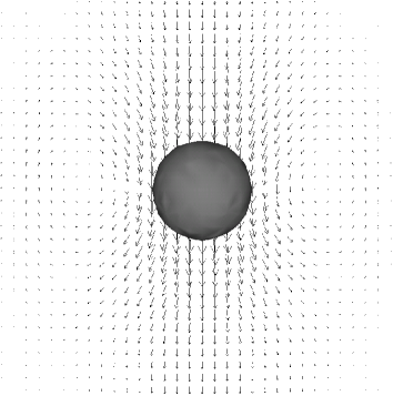
Figure 1: Snapshot of a sedimenting colloid of radius $a=4\Delta x$. The arrows indicate the velocity field.

Figure 2: Drag coefficient of a periodic array of spheres in steady Stokes flow as a function of volume fraction $\varphi$ solved using the SP method as compared with the analytic result zick82:_stokes  (Solid line) and low-$\varphi$ asymptotics hasimoto59:_stokes  (dashed line). In this case, $\xi$ is set to unity in the lattice unit. The range of the volume fraction $\varphi$ was obtained by changing the radius $a$ from $4$ to $15.5$ for a lattice size $\Delta x$ with $L=32\Delta x$ fixed.

To validate the SP method quantitatively, we measured the steady state drag force on a periodic array of spheres in a Newtonian solvent. The velocity distribution around the colloid is depicted in Fig.1. In general, flow around a colloid occurs as creep-flow with a Reynolds number of $Re=aV/\nu\ll 1$. Figure 2 shows the drag coefficient $Q(\varphi)$, defined as

$$F_{D} =-\frac{6\pi\eta aV}{Q(\varphi)},$$ (28)

where $\varphi=(4/3)\pi(a/L)^{3}$ is the volume fraction in a cubic box of volume $L^{3}$. The effect of the boundary condition extends very far in creep-flow, as the higher the volume fraction, the larger the drag. Comparison of the drag coefficient given by the SP method with the analytic result from the Stokes equation by Zick and Homsy zick82:_stokes verifies the validity of the SP method over the entire range of $\varphi$.

4.2 Lubrication interaction in a finite system

One of the most important effects of solvent flow is the lubrication interaction between nearby particles with relative motions. The exact solution of the Stokes equation for two isolated spheres has been found jeffrey84:_calcul_reynol and has provided much insight into the basic physics of colloidal suspensions. However, its application to many-particle systems through the method of pairwise addition requires care. For quantitative prediction of the rheology of concentrated suspensions, numerical results have identified many differences, whether the shear mode of the lubrication interaction is included or not ball97:_brown ; melrose04:_contin . There exists a fundamental ambiguity in the application of the analytic expression of two isolated spheres to a many-particle system in the finite domain using pairwise addition.

Figure 3: Snapshot of two approaching colloids of radius $a=4\Delta x$. The arrows indicate the velocity field. The color Map around the colloids represents the pressure distribution: a change in color from red to blue corresponds to a change from high to low pressure.

Figure 4: (a) Relative velocity between two approaching spheres versus the gap between the sphere surfaces (symbols). The slight oscillations in the SP results are a result of the finite lattice spacing. In this case, $\xi$ is set to unity in the lattice unit. Theoretical curves are shown for far-field asymptotics using the Rotne–Prager–Yamakawa tensor (dotted line) beenakker86:_ewald_rotne , a near-field exact solution (dashed line) jeffrey84:_calcul_reynol , and Stokesian Dynamics (solid line)brady88:_stokes_dynam . (b) The two coefficients representing the squeeze interaction (scaled to those at infinite dilution) versus volume fraction. $\gamma_{1}$ (square) represents the one-body drag and $\gamma_{2}$ (circle) represents the two-body squeeze interaction due to relative motion.

We computed the squeeze lubrication interaction between two approaching spheres in a finite system. The velocity and pressure distributions are depicted in Fig.3. Figure 4(a) shows the normalized approach velocity of a pair of particles versus the gap $h$ between two equal spheres solved by the SP method as compared with other theories. The two asymptotic solutions at $h\ll a$ and $h\gg a$ are from the exact solution of the isolated pair jeffrey84:_calcul_reynol and Rotne–Prager–Yamakawa tensor beenakker86:_ewald_rotne , respectively. The Stokesian Dynamics (SD) solution brady88:_stokes_dynam is based on an interpolation of these two asymptotic solutions. The simulation result nicely reproduces not only the two asymptotic regimes but also the crossover which occurs at $h/a\sim 0.7$. It is found that SD underestimates the mobility in this intermediate regime. This underestimation is due to the approximation adapted in SD in which the components are just asymptotic two-body solutions. The result confirms the relevance of our simulation, thus demonstrating the importance of the hydrodynamic interaction in a finite system.

We discuss the dependence of the lubrication interaction on the volume fraction. By assuming the functional form $\left|V_{1}-V_{2}\right|/F=1/\left(\Gamma_{1}(\varphi)+2\Gamma_{2}(\varphi)/h\right)$ from lubrication theory, where $\Gamma_{1}(\varphi)=6\pi\eta a\gamma_{1}(\varphi)$ is the one-body drag coefficient and $\Gamma_{2}(\varphi)=(3\pi\eta a^{2}/2)\gamma_{2}(\varphi)$ is the squeeze coefficient, the effect of the volume fraction is represented by $\gamma_{1}(\varphi)$ and $\gamma_{2}(\varphi)$. These friction coefficients can be extracted by fitting the curve of Fig.4(a) for each $\varphi$. The reduced coefficients $\gamma_{1}$ and $\gamma_{2}$ are plotted in Fig.4(b) as a function of the volume fraction. The solid line in Fig.4(b) is from Fig.2. Although a periodic array of spheres exhibits different flow geometry from the case of two approaching spheres, the volume fraction dependence of $\gamma_{1}$ of the two cases is comparable. Moreover, the squeeze coefficient $\gamma_{2}$ is found to be a decreasing function of the volume fraction. In other words, the squeeze mode is most enhanced at infinite dilution. In the literature kim91:_microh , it is pointed out that the squeeze coefficient is at least smaller than that of the exact solution for isolated pairs. These results further validate the SP method.

Although the SP method itself is an efficient scheme as a direct simulation of utility in constructing a more coarse-grained model for suspensions, such as in dissipative particle dynamics, constitutive modeling, etc., the calculation by direct simulation also gives fundamental information about the hydrodynamic interactions.

4.3 Sedimenting charged colloids

As an example of the specific application of the method to a multi-component fluid, we compute the hydrodynamic drag for sedimenting charged colloids in the absence of an external electric field. In this case, the sedimenting charged colloids induce a flow that determines a charge distribution which differs from the equilibrium case russel89:_colloid_disper ; probstein03:_physic_hydrod . The skewed ion-distribution gives rise to polarization in the electric double-layer. Moreover, double-layer deformation induces an electro-osmotic flow, which makes the flow around a charged colloid different from that of a neutral colloid.

In this simulation, a periodic array of charged colloids in a 1:1 electrolyte solution under gravity was computed. We specify the valence of the colloids first, and the counterion in the host fluid assures the charge neutrality of the whole system. The bulk concentrations of the 1:1 electrolyte $\bar{C}_{\pm}$ were determined by specifying the Debye length $\kappa^{-1}=\left\{4\pi\lambda_{B}(\bar{C}_{+}+\bar{C}_{-})\right\}^{-1/2}$. The Bjerrum length $4\pi\lambda_{B}=e^{2}/\epsilon k_{B}T$ was set to unity and $\xi$ was chosen as twice the lattice unit to resolve the surface charge distribution, which is represented by $\left|\nabla\phi\right|$. For simplicity, the counterion and coion were set to the Schmidt number $0.5$, which choice did not affect the qualitative aspect of the following results but only control the transient time to the steady state. The Debye length was chosen so that the effective radius of the double-layer $a+\kappa^{-1}$ was smaller than half of the system size $L/2$. In order to clarify the situation in terms of a typical colloid science parameter, nondimensional zeta potential $e\zeta/k_{B}T$ is shown in Fig.5, which should be determined by specifying $\kappa a$ and the valence of the colloid $Z$. The corresponding dimension of the zeta potential $\zeta$ for this simulation at 20^∘C is of the order of $10$mV. We computed the linear response regime for gravitational driving to observe the effect of electro-osmosis on hydrodynamic drag.

We plot the sedimentation velocity scaled by that of a neutral colloid as a function of the inverse Debye length scaled by the radius of colloid in Fig. 6. As the valence of the colloid or the zeta potential increases, the sedimentation velocity reduces to that of the neutral colloid. The hydrodynamic drag of the electrolyte solution was most enhanced when the Debye length was comparable to the size of the colloids. These facts qualitatively agree with the analytic result at infinite dilution booth54:_sedim_poten_veloc_solid_spher_partic ; ohshima84:_sedim_veloc_poten_dilut_suspen .

The charge-density and the velocity distributions when $\kappa a=1$ and $Z=1000$ are depicted in Fig.7. In this case, the charge distribution was largely uniform and thus the counteracting electrostatic effect of the double-layer polarization does not have much effect. Therefore, the enhanced electrohydrodynamic drag can mainly be attributed to the friction between the solvent and the ions. Because of this electrohydrodynamic coupling of the transfer in momentum, the solvent-flow pattern around the colloid was modified from the case of a neutral colloid. As a result, the viscous drag on the colloid was enhanced. This mechanism of enhanced viscous drag by electro-osmotic flow generally exists in colloids in electrolyte solutions.

It has been known that in an infinitely dilute system (or the thin double-layer limit) the velocity decays as $r^{-3}$ in the region of $\kappa r\gg 1$ in contrast to the $r^{-1}$ decay of an infinitely dilute neutral system, where $r$ is the radial distance from the center of the colloid anderson89:_colloid_trans_inter_forces ; long01 . However, in the system size adapted in our simulation this asymptotic regime was not reached. For $\kappa r\lesssim 1$, we have the screened hydrodynamics regime, where the velocity decays as $v\propto e^{-\kappa r}/r$ long01 .These factors account for why the flow patterns in Figs.(1) and (6) resemble one another. In other words, the electrohydrodynamic interaction should be a pronounced effect in small finite systems as is seen in neutral systems.

We note that, at a finite volume fraction and in the range of the Debye length, the charged colloid dynamics could be effectively assessed through the SP method. Further application of the SP method to electrophoresis of concentrated suspensions is reported elsewhere kim06:_direc_numer_simul_elect .

Figure 5: Non-dimensionalized zeta potential as a function of the inverse Debye length $\kappa a$ and the valence of the colloid $Z$ computed using the semi-analytic formula of Ohshima–Healy–White ohshima82:_accur . The dotted lines are guides to the eye.

Figure 6: Sedimentation velocity of a periodic array of colloids of different valences $Z$ in electrolyte solutions as a function of the inverse Debye length $\kappa a$. The ordinate is reduced by the sedimentation velocity of neutral colloids at the same volume fraction of $0.008$ ($a=4\Delta x,~{}L=32\Delta x$). The effective volume fraction including the electric double-layer defined by $(4/3)\pi\{(a+\kappa^{-1})/L\}^{3}$ was chosen to be less than unity. Dotted lines are guides to the eye.

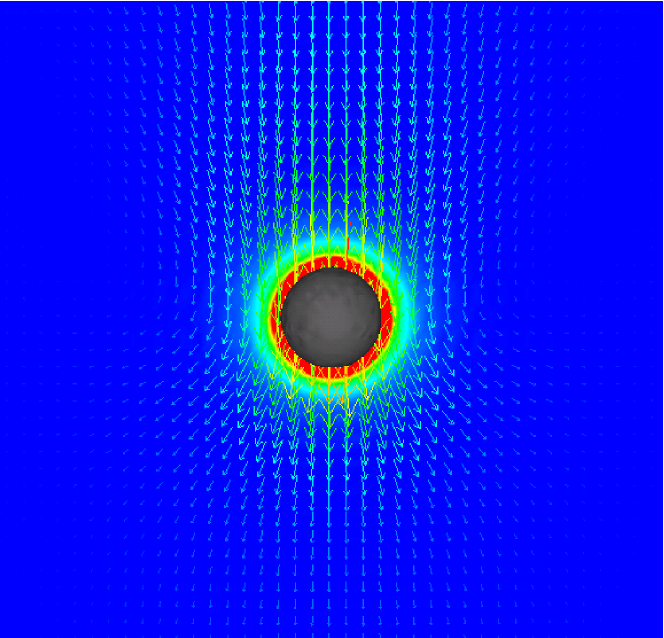
Figure 7: Snapshot of a sedimenting charged colloid when $\kappa a=1$ and $Z=1000$. The arrows indicate the velocity field. The color map around the particle represents the charge density field: a change in color from red to blue corresponds to a change from high to low charge density.

5 Conclusions

We have presented a new simulation scheme for colloidal dispersions in a solvent of a multi-component fluid, which we call the “Smoothed Profile (SP) method”. The SP method improves and extends a previous method proposed by the authors yamamoto01:_simul_partic_disper_nemat_liquid_cryst_solven ; nakayama05:_simul_method_resol_hydrod_inter_colloid_disper ; kim04:_effic .

The description of the colloidal systems is based on the Navier–Stokes equation for the momentum evolution of the solvent flow, the advection-diffusion equation for the solute distribution, the rigid body description of colloidal particles, with dynamical coupling of all these elements. Based on momentum conservation between the continuum solvent fluid and the discrete rigid colloids, the time-integrated hydrodynamic force and torque are derived. This expression of the mechanical coupling between a fluid and particles is well-suited for numerical simulations in which differential equations are discretized in time. With this formulation relating the solid-fluid interaction, standard discretization schemes for uniform fluids are utilized as is; no special care is needed for the solid-fluid boundary mesh. Since the hydrodynamic interaction is solved through direct simulation of the solvent fluid, the many-body effect can be fully resolved.

The utility of the SP method was assessed in various test problems, not only using simple fluids but also simulating charged colloids in electrolyte solutions. The results confirmed that the SP method is effective for studying the dynamical behavior of colloids. Although we have focused on systems of spherical colloids in simple fluids and Poisson–Nernst–Planck electrolytes (i.e. Poisson–Boltzmann level description of electrolytes), application to other types of macromolecules of other shapes, such as disks capuani06:_lattic_boltz , rods, and others, and other constitutive models for solvents is straightforward.

References

- (1) J. Happel, H. Brenner, Low Reynolds number hydrodynamics: with special applications to particulate media, 2nd edn. (Martinus Nijhoff, Dordrecht, 1983)
- (2) S. Kim, S.J. Karrila, Microhydrodynamics : principles and selected applications (Butterworth-Heinemann, London, 1991)
- (3) W.B. Russel, D.A. Saville, W.R. Schowalter, Colloidal Dispersions (Cambridge University Press, Cambridge, England, 1989)
- (4) C.N. Likos, Phys. Rep. 348, 267 (2001)
- (5) J.F. Brady, G. Bossis, Annu. Rev. Fluid Mech. 20, 111 (1988)
- (6) A. Malevanets, R. Kapral, J. Chem. Phys. 110, 8605 (1999)
- (7) H. Tanaka, T. Araki, Phys. Rev. Lett. 85, 1338 (2000)
- (8) T. Kajishima, S. Takiguchi, H. Hamasaki, Y. Miyake, JSME Int. J., Ser. B 44(4), 526 (2001)
- (9) H.H. Hu, N.A. Patankar, M.Y. Zhu, J. Comput. Phys. 192, 427 (2001)
- (10) R. Glowinski, T.W. Pan, T.I. Hesla, D.D. Joseph, J. Périaux, J. Comput. Phys. 192, 363 (2001)
- (11) A.J.C. Ladd, R. Verberg, J. Stat. Phys. 104, 1191 (2001)
- (12) J.T. Padding, A.A. Louis, Phys. Rev. Lett. 93, 220601 (2004)
- (13) M.E. Cates, K. Stratford, R. Adhikari, P. Stansell, J.C. Desplat, I. Pagonabarraga, A.J. Wagner, J. Phys.: Condens. Matter 16, S3903 (2004)
- (14) Y.W. Kim, R.R. Netz, Europhys. Lett. 72, 837 (2005)
- (15) T. Yamaue, M. Sasaki, T. Taniguchi, Multi-Phase Dynamics Program “Muffin” User’s Manual, http://octa.jp (2005)
- (16) V. Lobaskin, B. Dünweg, C. Holm, J. Phys.: Condens. Matter 16, S4063 (2004)
- (17) A. Chatterji, J. Horbach, J. Chem. Phys. 122, 184903 (2005)
- (18) F. Capuani, I. Pagonabarraga, D. Frenkel, J. Chem. Phys. 121, 973 (2004)
- (19) F. Capuani, I. Pagonabarraga, D. Frenkel, J. Chem. Phys. 124, 124903 (2006)
- (20) Y. Nakayama, R. Yamamoto, Phys. Rev. E 71, 036707 (2005)
- (21) L.D. Landau, E.M. Lifshitz, Fluid mechanics (Pergamon Press, London, 1959)
- (22) C.S. Peskin, D.M. McQueen, J. Comput. Phys. 81, 372 (1989)
- (23) J. Dzubiella, H. Löwen, C.N. Likos, Phys. Rev. Lett. 91, 248301 (2003)
- (24) H. Kodama, K. Takeshita, T. Araki, H. Tanaka, J. Phys.: Condens. Matter 16, L115 (2004)
- (25) A.A. Zick, G.M. Homsy, J. Fluid Mech. 115, 13 (1982)
- (26) H. Hasimoto, J. Fluid Mech. 5, 317 (1959)
- (27) D.J. Jeffrey, Y. Onishi, J. Fluid Mech. 139, 261 (1984)
- (28) R.C. Ball, J.R. Melrose, Physica A 247, 444 (1997)
- (29) J.R. Melrose, R.C. Ball, J. Rheol. 48, 937 (2004)
- (30) C.W. Beenakker, J. Chem. Phys. 85, 1581 (1986)
- (31) R.F. Probstein, Physicochemical Hydrodynamics : An Introduction, 2nd edn. (John Wiley & Sons, New York, 2003)
- (32) F. Booth, J. Chem. Phys. 22, 1956 (1954)
- (33) H. Ohshima, T.W. Healy, L.R. White, R.W. O’Brien, J. Chem. Soc., Faraday Trans. 2 80, 1299 (1984)
- (34) J.L. Anderson, Annu. Rev. Fluid Mech. 21, 61 (1989)
- (35) D. Long, A. Ajdari, Eur. Phys. J. E 4, 29 (2001)
- (36) K. Kim, Y. Nakayama, R. Yamamoto, Phys. Rev. Lett. 96, 208302 (2006)
- (37) H. Ohshima, T.W. Healy, L.R. White, J. Colloid Interface Sci. 90, 17 (1982)
- (38) R. Yamamoto, Phys. Rev. Lett. 87, 075502 (2001)
- (39) K. Kim, R. Yamamoto, Macromol. Theory Simul. 14, 278 (2005)