[

Heat transport of electron-doped Cobaltates

Abstract

Within the $t$-$J$ model, the heat transport of electron-doped cobaltates is studied based on the fermion-spin theory. It is shown that the temperature dependent thermal conductivity is characterized by the low temperature peak located at a finite temperature. The thermal conductivity increases monotonously with increasing temperature at low temperatures T $<$ 0.1$J$, and then decreases with increasing temperature for higher temperatures T $>$ 0.1$J$, in qualitative agreement with experimental result observed from Na_xCoO₂ .

]

The sodium cobalt oxide Na_xCoO₂ has become of considerable interest in the past few years because of its unconventional physical properties[1]. The structure of Na_xCoO₂ consists of triangular CoO₂ sheets separated by layers of Na⁺ ions[1, 2]. This structure is similar to cuprates in the sense that they also have a layered structure of the square lattice of the CuO₂ plane separated by insulating layers[3]. In the half-filling, the cobaltate is a Mott insulator, then the system becomes a strange metal by the electron doping[1, 2]. Moreover, superconductivity in the hydrated system Na_xCoO${}_{2}\cdot 1.3$H₂O has been observed in a narrow range of the electron doping concentration[4], around the optimal doping $x\approx 0.3$. Although the ferromagnetic correlation is present in Na_xCoO₂ for the large electron doping concentration ($x\approx 0.7$) [5], the antiferromagnetic (AF) short-range spin correlation in Na_xCoO₂ and Na_xCoO${}_{2}\cdot y$H₂O in the low electron doping concentration ($x\approx 0.35$) has been observed from the nuclear quadrupolar resonance and thermopower as well as other experimental measurements [6]. Therefore the unexpected finding of superconductivity in electron-doped cobaltate has raised the hope that it may help solve the unusual physics in doped cuprates.

The heat transport is one of the basic transport properties that provides a wealth of useful information on carriers and phonons as well as their scattering processes[7]. In the conventional metals, the thermal conductivity contains both contributions from carriers and phonons[7]. The phonon contribution to the thermal conductivity is always present in the conventional metals, while the magnitude of the carrier contribution depends on the type of materials because it is directly proportional to the free carrier density. However, the phonon contribution to the thermal conductivity is strongly suppressed for doped cuprates on a square lattice[8]. Moreover, an unusual contribution to the thermal conductivity of doped two-leg ladder materials has been observed[9], and this unusual contribution may be due to an energy transport via magnetic excitations[9]. Recently, the heat transport of the electron-doped cobaltate Na_xCoO₂ has been studied experimentally[10], where the behavior of the temperature dependent thermal conductivity is similar to the case of the doped two-leg ladder materials, and can not be explained within the conventional models of phonon heat transport based on phonon-defect scattering or conventional phonon-electron scattering. Within the charge-spin separation fermion-spin theory[11], the heat transports of doped cuprates on the square lattice and doped two-leg ladder materials have been studied[12, 13] based on the $t$-$J$ model, and the results are in agreement with experiments[8, 9]. Since the strong electron correlation is common for doped cuprates, two-leg ladder materials, and cobaltates, then these systems may have the same scattering mechanism that leads to the unusual heat transport. In this paper, we apply the charge-spin separation fermion-spin approach to study the heat transport of electron-doped cobaltates. Our results show that the thermal conductivity of the electron-doped cobaltate Na_xCoO₂ is characterized by the low temperature peak located at a finite temperature. Our results also show that although both dressed charge carriers and spin are responsible for the heat transport of electron-doped cobaltates, the contribution from the dressed spins are dominant.

As in the doped cuprates, the two-dimensional CoO₂ plane dominates the unconventional physics of electron-doped cobaltates. It has been argued that the essential physics of the doped CoO₂ plane can be described by the $t$-$J$ model on a triangular lattice [14],

$$H =- t\sum_{i\hat{\eta}\sigma}PC_{i\sigma}^{\dagger}C_{i+\hat{\eta}\sigma}P^{\dagger}-\mu\sum_{i\sigma}PC_{i\sigma}^{\dagger}C_{i\sigma}P^{\dagger}$$ (1)

$$+ J\sum_{i\hat{\eta}}{\bf S}_{i}\cdot{\bf S}_{i+\hat{\eta}},$$ (2)

where summation is over all site $i$, and for each $i$ over its nearest-neighbor $\hat{\eta}$, $C^{\dagger}_{i\sigma}$ ($C_{i\sigma}$) is the electron creation (annihilation) operator, ${\bf S}_{i}=C^{\dagger}_{i}{\bf\sigma}C_{i}/2$ is the spin operator with ${\bf\sigma}=(\sigma_{x},\sigma_{y},\sigma_{z})$ as the Pauli matrices, $\mu$ is the chemical potential, and the projection operator $P$ removes zero occupancy, i.e., $\sum_{\sigma}C^{\dagger}_{i\sigma}C_{i\sigma}\geq 1$. In order to use the charge-spin separation fermion-spin transformation[11], the $t$-$J$ model (1) can be rewritten in terms of a particle-hole transformation $C_{i\sigma}\rightarrow f^{\dagger}_{i-\sigma}$ as[15],

$$H=t\sum_{i\hat{\eta}\sigma}f_{i\sigma}^{\dagger}f_{i+\hat{\eta}\sigma}+\mu\sum_{i\sigma}f_{i\sigma}^{\dagger}f_{i\sigma}+J\sum_{i\hat{\eta}}{\bf S}_{i}\cdot{\bf S}_{i+\hat{\eta}},$$ (3)

then the original local constraint $\sum_{\sigma}C^{\dagger}_{i\sigma}C_{i\sigma}\geq 1$ is transferred as $\sum_{\sigma}f^{\dagger}_{i\sigma}f_{i\sigma}\leq 1$ to remove double occupancy, where $f^{\dagger}_{i\sigma}$ ($f_{i\sigma}$) is the hole creation (annihilation) operator, and ${\bf S}_{i}=f^{\dagger}_{i}{\bf\sigma}f_{i}/2$ is the spin operator in the hole representation. In this case, the hole operators can be expressed as $f_{i\uparrow}=a^{\dagger}_{i\uparrow}S^{-}_{i}$ and $f_{i\downarrow}=a^{\dagger}_{i\downarrow}S^{+}_{i}$ in the charge-spin separation fermion-spin representation[11], where the spinful fermion operator $a_{i\sigma}=e^{-i\Phi_{i\sigma}}a_{i}$ describes the charge degree of freedom together with some effects of the spin configuration rearrangements due to the presence of the doped charge carrier itself (dressed charge carrier), while the spin operator $S_{i}$ describes the spin degree of freedom (dressed spin), then the local constraint, $\sum_{\sigma}f^{\dagger}_{i\sigma}f_{i\sigma}=S^{+}_{i}a_{i\uparrow}a^{\dagger}_{i\uparrow}S^{-}_{i}+S^{-}_{i}a_{i\downarrow}a^{\dagger}_{i\downarrow}S^{+}_{i}=a_{i}a^{\dagger}_{i}(S^{+}_{i}S^{-}_{i}+S^{-}_{i}S^{+}_{i})=1-a^{\dagger}_{i}a_{i}\leq 1$, is satisfied in analytical calculations, and the double dressed charge carrier occupancy, $a^{\dagger}_{i\sigma}a^{\dagger}_{i-\sigma}=e^{i\Phi_{i\sigma}}a^{\dagger}_{i}a^{\dagger}_{i}e^{i\Phi_{i-\sigma}}=0$ and $a_{i\sigma}a_{i-\sigma}=e^{-i\Phi_{i\sigma}}a_{i}a_{i}e^{-i\Phi_{i-\sigma}}=0$, are ruled out automatically. It has been shown[11] that these dressed charge carrier and spin are gauge invariant, and in this sense, they are real and can be interpreted as the physical excitations. Although in common sense $a_{i\sigma}$ is not a real spinful fermion, it behaves like a spinful fermion. In this charge-spin separation fermion-spin representation, the low-energy behavior of the $t$-$J$ model (2) can be expressed as,

$$H = t\sum_{i\hat{\eta}}(a_{i\uparrow}S^{+}_{i}a^{\dagger}_{i+\hat{\eta}\uparrow}S^{-}_{i+\hat{\eta}}+a_{i\downarrow}S^{-}_{i}a^{\dagger}_{i+\hat{\eta}\downarrow}S^{+}_{i+\hat{\eta}})$$ (4)

$$- \mu\sum_{i\sigma}a^{\dagger}_{i\sigma}a_{i\sigma}+J_{{\rm eff}}\sum_{i\hat{\eta}}{\bf S}_{i}\cdot{\bf S}_{i+\hat{\eta}},$$ (5)

with $J_{{\rm eff}}=(1-\delta)^{2}J$, and $\delta=\langle a^{\dagger}_{i\sigma}a_{i\sigma}\rangle=\langle a^{\dagger}_{i}a_{i}\rangle$ is the electron doping concentration.

According to the linear response theory[16], the thermal conductivity can be obtained as,

$$\kappa(\omega,T)=-{1\over T}{{\rm Im}\Pi_{Q}(\omega,T)\over\omega},$$ (6)

with $\Pi_{Q}(\omega,T)$ is the heat current-current correlation function, and is defined as,

$$\Pi_{Q}(\tau-\tau^{\prime})=-\langle T_{\tau}j_{Q}(\tau)j_{Q}(\tau^{\prime})\rangle,$$ (7)

where $\tau$ and $\tau^{\prime}$ are the imaginary times, $T_{\tau}$ is the $\tau$ order operator, while the heat current density $j_{Q}$ is obtained within the Hamiltonian (3) by using Heisenberg’s equation of motion as [16],

$$j_{Q} = i\sum_{i,j}{\bf R}_{i}[H_{i},H_{j}]=j^{(f)}_{Q}+j^{(s)}_{Q},$$ (9)

$$j^{(f)}_{Q} = i(\chi t)^{2}\sum_{i\hat{\eta}\hat{\eta}^{\prime}\sigma}\hat{\eta}a_{i+\hat{\eta}^{\prime}\sigma}^{\dagger}a_{i+\hat{\eta}\sigma}-i\mu\chi t\sum_{i\hat{\eta}\sigma}\hat{\eta}a_{i+\hat{\eta}\sigma}^{\dagger}a_{i\sigma},$$ (10)

$$j^{(s)}_{Q} = i{1\over 2}(\epsilon J_{\rm{eff}})^{2}\sum_{i\hat{\eta}\hat{\eta}^{\prime}}(\hat{\eta}-\hat{\eta}^{\prime})[S^{+}_{i}S^{-}_{i-\hat{\eta}+\hat{\eta}^{\prime}}S^{z}_{i-\hat{\eta}}$$ (11)

$$+ S^{-}_{i-\hat{\eta}+\hat{\eta}^{\prime}}S^{+}_{i}S^{z}_{i-\hat{\eta}}]+i\epsilon J^{2}_{\rm{eff}}\sum_{i\hat{\eta}\hat{\eta}^{\prime}}(\hat{\eta}-\hat{\eta}^{\prime})[S^{+}_{i}S^{-}_{i+\hat{\eta}}S^{z}_{i+\hat{\eta}^{\prime}}$$ (12)

$$- S^{+}_{i}S^{-}_{i-\hat{\eta}}S^{z}_{i-\hat{\eta}+\hat{\eta}^{\prime}}],$$ (13)

where ${\bf R}_{i}$ is lattice site, the spin correlation function $\chi=\langle S_{i}^{+}S_{i+\hat{\eta}}^{-}\rangle$, $\epsilon=1-2t\phi/J_{\rm eff}$, and the dressed charge carrier particle-hole parameter $\phi=\langle a^{\dagger}_{i\sigma}a_{i+\hat{\eta}\sigma}\rangle$. Within the $t$-$J$ model, the thermal conductivity of hole-doped cuprates on the square lattice has been obtained[12]. Following their discussions, the thermal conductivity of electron-doped cobaltates on the triangular lattice can be obtained as,

$$\kappa(\omega,T) = \kappa_{f}(\omega,T)+\kappa_{s}(\omega,T),$$ (15)

$$\kappa_{f}(\omega,T) = -{1\over 2N}\sum_{k\sigma}\Lambda_{f}^{2}\gamma^{2}_{sk}\int^{\infty}_{-\infty}{d\omega^{\prime}\over 2\pi}A_{f\sigma}(k,\omega^{\prime}+\omega)$$ (16)

$$\times A_{f\sigma}(k,\omega^{\prime}){n_{F}(\omega^{\prime}+\omega)-n_{F}(\omega^{\prime})\over T\omega},$$ (17)

$$\kappa_{s}(\omega,T) = -{1\over 2N}\sum_{k}\Lambda_{s}^{2}\gamma^{2}_{sk}\int^{\infty}_{-\infty}{d\omega^{\prime}\over 2\pi}A_{s}(k,\omega^{\prime}+\omega)$$ (18)

$$\times A_{s}(k,\omega^{\prime}){n_{B}(\omega^{\prime}+\omega)-n_{B}(\omega^{\prime})\over T\omega},$$ (19)

where $\Lambda_{f}=-Z\chi t(\mu+Z\chi t\gamma_{k})$, $\Lambda_{s}=(ZJ_{{\rm eff}})^{2}\epsilon(2\epsilon\chi+2C-4\chi\gamma_{k})$, $\gamma_{sk}^{2}=\{[{\rm sin}k_{x}+{\rm sin}(k_{x}/2){\rm cos}({\sqrt{3}}k_{y}/2)]^{2}+3[{\rm sin}({\sqrt{3}}k_{y}/2){\rm cos}(k_{x}/2)]^{2}\}/9$, $\gamma_{k}=[{\rm cos}(k_{x})+2{\rm cos}(k_{x}/2){\rm cos}({\sqrt{3}}k_{y}/2)]/3$,the spin spectral function $A_{s}(k,\omega)=-2{\rm Im}D(k,\omega)$, the dressed charge carrier spectral function $A_{f\sigma}(k,\omega)=-2{\rm Im}g_{\sigma}(k,\omega)$, and $n_{F}(\omega)$ and $n_{B}(\omega)$ are the fermion and boson distribution functions, respectively, while the full dressed charge carrier and spin Green’s functions are evaluated as,

$$g^{-1}_{\sigma}(k,\omega)={1\over g^{(0)-1}_{\sigma}(k,\omega)-\Sigma_{f}(k,\omega)},$$ (21)

$$D^{-1}(k,\omega)={1\over D^{(0)-1}(k,\omega)-\Sigma_{s}(k,\omega)},$$ (22)

respectively, where the mean-field (MF) dressed charge carrier Green’s function $g^{(0)-1}_{\sigma}(k,\omega)=\omega-\xi_{k}$, the MF spin Green’s function $D^{(0)-1}(k,\omega)=(\omega^{2}-\omega_{k}^{2})/B_{k}$, with $B_{k}=\lambda[2\chi^{z}(\epsilon\gamma_{k}-1)+\chi(\gamma_{k}-\epsilon)]$, $\lambda=2ZJ_{eff}$, the spin correlation function $\chi^{z}=\langle S_{i}^{z}S_{i+\hat{\eta}}^{z}\rangle$, and the MF dressed charge carrier and spin excitation spectra are given by,

$$\xi_{k} = -Zt\chi\gamma_{k}-\mu,$$ (24)

$$\omega^{2}_{k} = A_{1}(\gamma_{k})^{2}+A_{2}\gamma_{k}+A_{3},$$ (25)

respectively, where $A_{1}=\alpha\epsilon\lambda^{2}(\epsilon\chi^{z}+\chi/2)$, $A_{2}=-\epsilon\lambda^{2}[\alpha(\chi^{z}+\epsilon\chi/2)+(\alpha C^{z}+(1-\alpha)/(4Z)-\alpha\epsilon\chi/(2Z))+(\alpha C+(1-\alpha)/(2Z)-\alpha\chi^{z}/2)/2]$, $A_{3}=\lambda^{2}[\alpha C^{z}+(1-\alpha)/(4Z)-\alpha\epsilon\chi/(2Z)+\epsilon^{2}(\alpha C+(1-\alpha)/(2Z)-\alpha\chi^{z}/2)/2]$, the spin correlation functions $C=(1/Z^{2})\sum_{\hat{\eta},\hat{\eta^{\prime}}}\langle S_{i+\hat{\eta}}^{+}S_{i+\hat{\eta^{\prime}}}^{-}\rangle$, $C^{z}=(1/Z^{2})\sum_{\hat{\eta},\hat{\eta^{\prime}}}\langle S_{i+\hat{\eta}}^{z}S_{i+\hat{\eta^{\prime}}}^{z}\rangle$, while the second-order dressed charge carrier and spin self-energy functions are evaluated by the loop expansion to the second-order as,

$$\Sigma_{f}(k,\omega)={1\over 2}\left({Zt\over N}\right)^{2}\sum_{pp^{\prime}}(\gamma^{2}_{p^{\prime}+p+k}+\gamma^{2}_{p^{\prime}-k}){B_{p^{\prime}}B_{p+p^{\prime}}\over 4\omega_{p^{\prime}}\omega_{p+p^{\prime}}}$$ (27)

$$\times \left({F^{(h)}_{1}(k,p,p^{\prime})\over\omega+\omega_{p+p^{\prime}}-\omega_{p^{\prime}}-\xi_{p+k}}+{F^{(h)}_{2}(k,p,p^{\prime})\over\omega+\omega_{p^{\prime}}-\omega_{p+p^{\prime}}-\xi_{p+k}}\right.$$ (28)

$$+ \left.{F^{(h)}_{3}(k,p,p^{\prime})\over\omega+\omega_{p^{\prime}}+\omega_{p+p^{\prime}}-\xi_{p+k}}-{F^{(h)}_{4}(k,p,p^{\prime})\over\omega-\omega_{p+p^{\prime}}-\omega_{p^{\prime}}-\xi_{p+k}}\right),$$ (29)

$$\Sigma_{s}(k,\omega)=\left({Zt\over N}\right)^{2}\sum_{pp^{\prime}}(\gamma^{2}_{p^{\prime}+p+k}+\gamma^{2}_{p^{\prime}-k}){B_{k+p}\over 2\omega_{k+p}}$$ (31)

$$\times \left({F^{(s)}_{1}(k,p,p^{\prime})\over\omega+\xi_{p+p^{\prime}}-\xi_{p^{\prime}}-\omega_{k+p}}-{F^{(s)}_{2}(k,p,p^{\prime})\over\omega+\xi_{p+p^{\prime}}-\xi_{p^{\prime}}+\omega_{k+p}}\right),$$ (32)

respectively, where $F^{(h)}_{1}(k,p,p^{\prime})=n_{F}(\xi_{p+k})[n_{B}(\omega_{p^{\prime}})-n_{B}(\omega_{p+p^{\prime}})]+n_{B}(\omega_{p+p^{\prime}})[1+n_{B}(\omega_{p^{\prime}})]$, $F^{(h)}_{2}(k,p,p^{\prime})=n_{F}(\xi_{p+k})[n_{B}(\omega_{p^{\prime}+p})-n_{B}(\omega_{p^{\prime}})]+n_{B}(\omega_{p^{\prime}})[1+n_{B}(\omega_{p^{\prime}+p})]$, $F^{(h)}_{3}(k,p,p^{\prime})=n_{F}(\xi_{p+k})[1+n_{B}(\omega_{p+p^{\prime}})+n_{B}(\omega_{p^{\prime}})]+n_{B}(\omega_{p^{\prime}})n_{B}(\omega_{p+p^{\prime}})$, $F^{(h)}_{4}(k,p,p^{\prime})=n_{F}(\xi_{p+k)}[1+n_{B}(\omega_{p+p^{\prime}})+n_{B}(\omega_{p^{\prime}})]-[1+n_{B}(\omega_{p^{\prime}})][1+n_{B}(\omega_{p+p^{\prime}})]$, $F^{(s)}_{1}(k,p,p^{\prime})=n_{F}(\xi_{p+p^{\prime}})[1-n_{F}(\xi_{p^{\prime}})]-n_{B}(\omega_{k+p})[n_{F}(\xi_{p^{\prime}})-n_{F}(\xi_{p+p^{\prime}})]$, and $F^{(s)}_{2}(k,p,p^{\prime})=n_{F}(\xi_{p+p^{\prime}})[1-n_{F}(\xi_{p^{\prime}})]+[1+n_{B}(\omega_{k+p})][n_{F}(\xi_{p^{\prime}})-n_{F}(\xi_{p+p^{\prime}})]$. In order not to violate the sum rule of the correlation function $\langle S^{+}_{i}S^{-}_{i}\rangle=1/2$ in the case without AF long-range order, the important decoupling parameter $\alpha$ has been introduced in the MF calculation [17], which can be regarded as the vertex correction, then all the above MF order parameters, decoupling parameter $\alpha$, and chemical potential $\mu$ are determined by the self-consistent calculation [18].

We are now ready to discuss the heat transport of electron-doped cobaltates. The observable temperature dependence of thermal conductivity $\kappa(T)$ in the experiments can be obtained from Eq. (7a) as $\kappa(T)=\lim_{\omega\rightarrow 0}\kappa(\omega,T)$. We have performed the numerical calculation for this thermal conductivity $\kappa(T)$, and the results of $\kappa(T)$ at the electron doping concentration $x=0.31$ (solid line), and $x=0.33$ (dotted line) for $t/J=2.5$ are shown in Fig. 1. For the comparison, the experimental result[10] taken from Na_3.1CoO₂ is also shown in Fig. 1(inset). Our results show that the thermal conductivity $\kappa(T)$ increases monotonously with increasing temperatures for the low-temperature range $T<0.1J$, and reaches at the peak position in the temperature $T\approx 0.1J$, then decreases with increasing temperatures for the higher temperature range $T>0.1J$. Using a reasonable estimation value of $J\approx 300$ to $500k$ in Na_xCoO₂, the position of the peak is at $T\approx 0.1J\approx 30\sim 50k$. These results are in qualitative agreement with the experimental data [10].

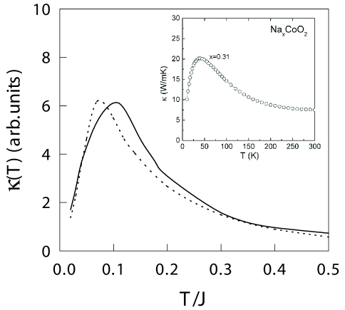
FIG. 1.: The thermal conductivity $\kappa(T)$ as a function of temperature at the electron doping concentration x = 0.31 (solid line) and x = 0.33 (dotted line) with $t/J=2.5$.

During the above calculation, we have found as in doped cuprates[12] that although both dressed charge carriers and spin are responsible for the thermal conductivity $\kappa(T)$, the contribution from the dressed spins is much larger than these from the dressed charge carriers, i.e., $\kappa_{s}(T)\gg\kappa_{f}(T)$ in electron-doped cobaltates, and therefore the thermal conductivity of electron-doped cobaltates is mainly determined by its dressed spin part $\kappa_{s}(T)$. In this case, the physical interpretation of the present results is the same as in the case of doped cuprates[12], i.e., the observed unusual thermal conductivity of electron-doped cobaltates is closely related to the incommensurate spin response in the systems[19, 20]. Since $\kappa_{s}(\omega,T)$ in Eq. (7c) is obtained in terms of the dressed spin Green’s function $D(k,\omega)$, while the dynamical spin structure factor of doped Mott insulators on the triangular lattice has been obtained from the dressed spin Green’s function as[19, 20],

$$S(k,\omega) = -2[1+n_{B}(\omega)]{\rm Im}D(k,\omega)$$ (34)

$$= -2[1+n_{B}(\omega)]B_{k}{\rm Im}\Sigma_{s}(k,\omega)\over[\omega^{2}-\omega^{2}_{k}-{\rm Re}\Sigma_{s}(k,\omega)]^{2}+[{\rm Im}\Sigma_{s}(k,\omega)]^{2},$$ (35)

where ${\rm Im}\Sigma_{s}(k,\omega)$ and ${\rm Re}\Sigma_{s}(k,\omega)$ are corresponding imaginary part and real part of the dressed spin self-energy function $\Sigma_{s}(k,\omega)$ in Eq. (10b). As we have shown in detail in Ref. [19,20], the dynamical spin structure factor (11) has a well-defined resonance character. $S(k,\omega)$ exhibits a peak when the incoming neutron energy $\omega$ is equal to the renormalized spin excitation $E^{2}_{k}=\omega^{2}_{k}+B_{k}{\rm Re}\Sigma_{s}(k,E_{k})$ for certain critical wave vectors $k_{\delta}$ (positions of the incommensurate peaks), then the height of these peaks is determined by the imaginary part of the dressed spin self-energy function ${\rm Im}\Sigma_{s}(k_{\delta},\omega)$. Since the time scale of this dynamical incommensurate correlation is comparable to that of lattice vibrations as in the case of the square lattice[12], then this dynamical spin modulations dominate the heat transport of electron-doped cobaltates, i.e., energy transport via magnetic excitations dominates the thermal conductivity. On the other hand, the dynamical spin response is doping dependent, this leads to the thermal conductivity of electron-doped cobaltates also is doping dependent.

In summary, we have studied the heat transport of electron-doped cobaltates within the $t$-$J$ model. Our results show that the thermal conductivity of electron-doped cobaltates is characterized by the low temperature peak located at a finite temperature. The thermal conductivity increases monotonously with increasing temperatures at low temperature range $T<0.1J$, and decreases with increasing temperatures at higher temperature range $T>0.1J$. Our results are in qualitative agreement with the experimental data of Na_xCoO₂.

REFERENCES

• [1] I. Terasaki, Y. Sasago, and K. Uchinokura, Phys. Rev. B 56, R12685 (1997).
• [2] M. Von Jansen and R. Hoppe, Z. Anorg. Allg. Chem. 408, 104 (1974).
• [3] M. A. Kastner, R. J. Birgeneau, G. Shiran, Y. Endoh, Rev. Mod. Phys. 70, 897 (1998).
• [4] K. Takada, H. Sakurai, E. Takayama-Muromachi, F. Izumi, R.A. Dilanian, and T. Sasaki, Nature 422, 53 (2003).
• [5] T. Motohashi, R. Ueda, E. Naujalis, T. Tojo, I. Terasaki, T. Atake, M. Karppinen, and H. Yamauchi, Phys. Rev. B 67, 064406 (2003).
• [6] R.E. Schaak, T. Klimczuk, M.L. Foo, and R.J. Cava, Nature 424, 527 (2003); A. Kanigel, A. Keren, L. Patlagan, K.B. Chashka, B. Fisher, P. King, and A. Amato, cond-mat/0311427; Y.J. Uemura, P.L. Russo, A.T. Savici, C.R. Wiebe, G.J. MacDougall, G.M. Luke, M. Mochizuki, Y. Yanase, M. Ogata, M.L. Foo, and R.J. Cava, cond-mat/0403031; T. Fujimoto, G.Q. Zheng, Y. Kitaoka, R.L. Meng, J. Cmaidalka, and C.W. Chu, Phys. Rev. Lett. 92, 047004 (2004); Yayu Wang, N.S. Rogado, R.J. Cava, and N.P. Ong, Nature 423, 425 (2003).
• [7] C. Uher, in Physics Properties of High Temperature Superconductivity III, Edited by D. M. Ginsberg (World Scientific, Singapore, 1992), P159.
• [8] Y. Nakamura, S. Uchida, T. Kimura, N. Motohira, K. Kishio, K. Kitazawa, T. Arima, Y. Tokura, Physica C 185-189, 1409 (1991); O. Baberski, A. Lang, O. Maldonado, M. Hücker, B. Büchner, A. Freimuth, Europhys. Lett. 44, 335 (1998).
• [9] A. V. Sologubenko, K. Gianno, H. R. Ott, and A. Revcolevschi, Phys. Rev. Lett 84, 2714 (2000); C. Hess, C. Baumann, U. Ammerahl, B. Buchner, F. Heidrich-Meisner, W. Bvenig, and A. Revcolevschi, Phys. Rev. B 64, 184305 (2001); F. Heidrich-Meisner, A. Honecher, D. C. Cabra, W. Brenig, Phys. Rev. B 66, 140406 (2002); K. Kudo, S. Ishikawa, T. Noji, Y. Koike, K. Maki, S. Tsuji, and Ken-ichi Kumagai, J. Phys. Soc. Jpn. 70, 437 (2001).
• [10] M.L. Foo, Yayu Wang, S. Watauchi, H.W. Zandbergen, Tao He, R.J. Cava, and N.P. Ong, Phys. Rev. Lett. 92, 247001 (2004).
• [11] Shiping Feng, Jihong Qin, and Tianxing Ma, J. Phys. Condens. Matter 16, 343 (2004); Shiping Feng, Tianxing Ma, and Jihong Qin, Mod. Phys. Lett. B 17, 361 (2003).
• [12] Tianxing Ma and Shiping Feng, Phys. Lett. A 328, 212 (2004).
• [13] Jihong Qin, Shiping Feng, Feng Yuan, and Wei Yeu Chen, Phys. Lett. A 335, 477 (2005).
• [14] G. Baskaran, Phys. Rev. Lett. 91, 097003 (2003).
• [15] Bin Liu, Ying Liang, Shiping Feng, and Wei Yeu Chen, Phys. Rev. B 69, 224506 (2004); Bin Liu, Ying Liang, Shiping Feng, and Wei Yeu Chen, Commun. Theor. Phys 43, 1127 (2005); Bin Liu, Ying Liang, and Shiping Feng, Int. J. Mod. Phys. B 19, 73(2005).
• [16] G.D. Mahan, Many-Particle Physics , Plenum Press, New York, 1990.
• [17] J. Kondo and K. Yamaji, Prog. Theor. Phys. 47, 807 (1972).
• [18] Shiping Feng and Yun Song, Phys. Rev. B 55, 642 (1997).
• [19] Ying Liang and Shiping Feng, Phys. Lett. A 296, 301 (2002); Ying Liang, Tianxing Ma, and Shiping Feng, Commun. Theor. Phys 39, 749 (2003).
• [20] Bin Liu, Ying Liang, Shiping Feng, and Wei Yeu Chen, unpublished.