Hahn echo and criticality in spin-chain systems

Abstract

We establish a relation between Hahn spin-echo of a spin-$\frac{1}{2}$ particle and quantum phase transitions in a spin-chain, which couples to the particle. The Hahn echo is calculated and discussed at zero as well as at finite temperatures. On the example of XY model, we show that the critical points of the chain are marked by the extremal values in the Hahn echo, and can influence the Hahn echo in finite temperatures. An explanation for the relation between the echo and criticality is also presented.

Quantum phase transitionssachdev99 (QPTs) have attracted enormous attention within various fields of physics in the past decade. They exist on all length scales, from microscopic to macroscopic. Because QPTs, which describe transitions between quantitatively distinct phases, are driven solely by quantum fluctuations, they provide valuable information about the ground state and nearby excited states of quantum many-body systems. The observation of quantum criticality depends eventually on the experimentally available temperature, then it is natural to ask how high in temperature can the effects of quantum criticality persist? Do quantum critical points shed light on quantum mechanics of macroscopic systems, for instance providing a deeper understanding of decoherence? In this paper we answer these questions by examining exact solutions of the XY spin-chain model, calculating the Hahn echo of a spin-$1/2$ particle coupled to the critical spin-chain.

The Hahn echo was first introduced by Hahnhahn50 to observe and measure directly transverse relaxation time $T_{2}$, i.e., the dephasing time. It differentiates from the Loschmidt echo in that the latter measures the sensitivity of quantum system dynamics to perturbations in the Hamiltonian. For a certain regime of parameters, the Loschmidt echo decays exponentially with a rate given by the Lyapunov exponent of the underlying classically chaotic system. Recently, a huge interest was attracted in the attempt of characterizing QPTs in terms of entanglement, by analyzing extremal points, scaling and asymptotic behavior in various entanglement measuresosterloh02 ; vidal03 ; wu04 ; chen04 ; gu05 . The relation between Berry’s phases and quantum critical points was also established recently in the XY modelcarollo05 ; zhu05 ; hamma06 . In this paper, we shall show how critical points can be reflected in the Hahn spin-echo, and what is the finite temperature effect on the Hahn spin-echo.

Consider a spin-$1/2$ particle coupled to a spin-chain described by the one-dimensional XY model, the Hamiltonian of such a system may be given by

$$H=H_{s}+H_{c}+H_{i},$$ (1)

where

$$H_{s} = \mu s^{z},$$

$$H_{c} = -2\sum_{l=1}^{N}((1+\gamma)s_{l}^{x}s_{l+1}^{x}+(1-\gamma)s_{l}^{y}s_{l+1}^{y}+\lambda s_{l}^{z}),$$

$$H_{i} = 4g\sum_{l=1}^{N}s^{z}s_{l}^{z}.$$ (2)

Here $s$ denotes spin operator of the system particle which couples to the chain spins $s_{l}$ $(l=1,...,N)$ located at the lattice site $l$. The spins in the chain are coupled to the system particle through a constant $g$. The Hahn echo experiments consists in preparing the system spin in the initial state $|y_{s}\rangle=(|\uparrow\rangle+i|\downarrow\rangle)/\sqrt{2}$, and then allowing free evolution for time $\tau$. A $\pi$-pulse described by the Pauli operator $\sigma^{x}$ is then applied to the system spin, and after free evolution for one more interval $\tau$ an echo is observed, which provides a direct measurement of single spin coherence. We would like to notice that the free evolution here means no additional driving fields exist, the coupling between the system and the spin-chain is always there.

We now follow the calculationwitzel05 to derive an exact expression for the Hahn echo decay due to the system-chain couplings in Eq.(1). The density matrix for the whole system (system and the spin-chain) which will be used to calculate the Hahn echo is given by

$$\rho(\tau)=U(\tau)\rho_{0}U^{\dagger}(\tau),$$ (3)

where $U(\tau)$ denotes the evolution operatorwitzel05

$$U(\tau)=u(\tau)\sigma^{x}u(\tau),u(\tau)=e^{-iH\tau},$$ (4)

and $\rho_{0}$ is taken to be the initial state of the whole system

$$\rho_{0}=|y_{s}\rangle\langle y_{s}|\otimes\rho_{c}(0)$$ (5)

with $\rho_{c}(0)$ denoting the initial state for the spin-chain. The Hahn spin echo envelope is then given by

$$v_{E}(\tau)=2|{\mbox{T}r}\{(s^{x}+is^{y})\rho(\tau)\}|.$$ (6)

In order to get an explicit expression for the Hahn echo envelope Eq.(6), we first write $u(\tau)$ in basis $\{|\uparrow\rangle,|\downarrow\rangle\}$ (the eigenstates of $\sigma^{z}$), by noting that $[H_{s},H_{i}]=0.$ This leads to

$$u(\tau)=\sum_{j=\uparrow,\downarrow}u_{j}(\tau)|j\rangle\langle j|,$$ (7)

with $u_{j}(\tau)$ satisfying,

$$i\hbar\frac{\partial}{\partial t}u_{j}(t)=H_{j}u_{j}(t),$$

$$H_{j}=-2\sum_{l=1}^{N}((1+\gamma)s_{l}^{x}s_{l+1}^{x}+(1-\gamma)s_{l}^{y}s_{l+1}^{y}+\lambda_{j}s_{l}^{z}),$$ (8)

where $\lambda_{j}=\lambda\pm g$, $+$ and $-$ correspond to $\downarrow$ and $\uparrow$, respectively. The free energy $\mu$ of the system which contributes only energy shifts to $H_{j}$ would not affect the Hahn echo and has been omitted hereafter. For the system initially in state $|j\rangle$ $(j=\uparrow,\downarrow)$, the dynamics and statistical properties of the spin-chain would be govern by $H_{j}$, it takes the same form as $H_{c}$ but with perturbed field strengths $\lambda_{j}$. This perturbation to the spin-chain regardless of how small it is can be reflected in the Loschmidt spin echo decay quan05 , in particular at critical points. What behind the decay is the orthogonalization between two ground states obtained for two different values of external parameterszanardi05 . The Hamiltonian $H_{j}$ can be diagonalized by a standard procedure to be

$$H_{j}=\sum_{k}\omega_{j,k}(\eta_{j,k}^{\dagger}\eta_{j,k}-\frac{1}{2}),$$ (9)

which can be summarized in the following three steps. (1) The Wigner-Jordan transformation, which converts the spin operators into fermionic operators via the relation $a_{l}=(\prod_{m<l}\sigma_{m}^{z})(\sigma_{l}^{x}+i\sigma_{l}^{y})/2$, where $\sigma_{l}$ is the Pauli matrix of the spin at site $l$; (2)The Fourier transformation, $d_{k}=\frac{1}{\sqrt{N}}\sum_{l}a_{l}\mbox{exp}(-i2\pi lk/N);$ And (3) the Bogoliubov transformation, which defines the fermionic operators,

$$\eta_{j,k}=d_{k}\cos\frac{\theta_{j,k}}{2}-id_{-k}^{\dagger}\sin\frac{\theta_{j,k}}{2},$$ (10)

where the mixing angle $\theta_{j,k}$ was defined by $\cos\theta_{j,k}=\varepsilon_{j,k}/\omega_{j,k},$ with $\omega_{j,k}=\sqrt{\varepsilon_{j,k}^{2}+\gamma^{2}\sin^{2}\frac{2\pi k}{N}},$ and $\varepsilon_{j,k}=(\cos\frac{2\pi k}{N}-\lambda_{j}),$ $k=-N/2,-N/2+1,...,N/2-1.$ To diagonalize the spin chain Hamiltonian, the periodic boundary condition was used in this paper. The boundary term $H_{b}=-(a^{\dagger}_{1}a_{N}+a_{N}^{\dagger}a_{1}+\gamma(a_{N}^{\dagger}a_{1}^{\dagger}+h.c.))(P+1)$ with $P=exp(i\pi\sum_{j=1}^{N}a_{j}^{\dagger}a_{j})$ would vanish when $N/2$ is odd. Since the paper aims at finding the link between the Hahn echo and the critical points, we will chose $N/2$ odd to simplify the boundary effects. This treatment is available in the limit $N\rightarrow\infty$, where the boundary effects are negligible. It is easy to show that $[\eta_{i,k},\eta_{j,k}]\neq 0$ when $j\neq i$, i.e., the modes $\eta_{i,k}$ and $\eta_{j,k}$ do not commute(this is not the case for some special parameters discussed later on). This would result in the Hahn echo decay as you will see. With these results, the evolution operator $U(\tau)$ can be reduced to

$$U(\tau)=u_{\uparrow}(\tau)u_{\downarrow}(\tau)|\uparrow\rangle\langle\downarrow|+u_{\downarrow}(\tau)u_{\uparrow}(\tau)|\downarrow\rangle\langle\uparrow|,$$ (11)

with $u_{j}(\tau)=e^{-i\sum_{k}\omega_{j,k}(\eta_{j,k}^{\dagger}\eta_{j,k}-\frac{1}{2})\tau}\equiv\prod_{k}u_{j,k}(\tau)$, $j=\uparrow,\downarrow,$ and $u_{j,k}(\tau)=e^{-i\omega_{j,k}(\eta_{j,k}^{\dagger}\eta_{j,k}-\frac{1}{2})\tau}.$ After a simple algebra, we arrive at

$$v_{E}(\tau)=|{\mbox{T}r_{c}}(u^{\dagger}_{\downarrow}u^{\dagger}_{\uparrow}u_{\downarrow}u_{\uparrow}\rho_{c}(0))|,$$ (12)

where the trace is taken over the spin-chain. Eq.(12) can be simplified by noting that ($n_{j,k}=\eta_{j,k}^{\dagger}\eta_{j,k}$)

$$[n_{\uparrow,k},n_{\downarrow,k}]=\frac{i}{2}\sin(\theta_{\uparrow,k}-\theta_{\downarrow,k})(\eta_{-k}\eta_{k}-\eta_{k}^{\dagger}\eta_{-k}^{\dagger}),$$ (13)

and consequently,

$$u^{\dagger}_{\uparrow,k}u_{\downarrow,k}=u_{\downarrow,k}u^{\dagger}_{\uparrow,k}+\hat{X}_{k},$$ (14)

where $\hat{X}_{k}=(1-e^{i\omega_{\uparrow,k}t})(1-e^{-i\omega_{\downarrow,k}t})[n_{\uparrow,k},n_{\downarrow,k}]$. Here $\eta_{k}=d_{k}\cos\frac{\theta_{k}}{2}-id_{-k}^{\dagger}\sin\frac{\theta_{k}}{2},$ and $\theta_{k}=\theta_{j,k}|_{\lambda_{j}=\lambda}.$ Substituting Eq.(14) into $v_{E}(\tau)$, we get

$$v_{E}(\tau)=\prod_{k}|1+{\mbox{T}r_{c}}[u^{\dagger}_{\downarrow,k}\hat{X}_{k}u_{\uparrow,k}\rho_{c}(0)]|.$$ (15)

The explicit expression for Eq.(15) can be obtained by choosing a specific initial state of the chain. We shall consider two initial states in this paper, (1) $\rho_{c}(0)$ is taken to be the ground state of $H_{c}$, (2) $\rho_{c}(0)$ is chosen to be a thermal state for the spin-chain. The ground state of $H_{c}$ follows by the same steps summarized above. It is defined as the state to be annihilated by each operator $\eta_{k}$, namely $\eta_{k}|g(\gamma,\lambda)\rangle=0.$ After a few manipulations we obtain the Hahn echo envelope at zero temperature,

$$v_{E}(t) = \prod_{k}|1+\frac{1}{4}\sin(\theta_{\uparrow,k}-\theta_{\downarrow,k})\sin(\theta_{k}-\theta_{\uparrow,k})|1-e^{i\omega_{\uparrow,k}t}|^{2}(1-e^{-i\omega_{\downarrow,k}t}-\sin^{2}\frac{\theta_{k}-\theta_{\downarrow,k}}{2}|1-e^{i\omega_{\downarrow,k}t}|^{2})$$ (16)

$$- \frac{1}{4}\sin(\theta_{\uparrow,k}-\theta_{\downarrow,k})\sin(\theta_{k}-\theta_{\downarrow,k})|1-e^{i\omega_{\downarrow,k}t}|^{2}(1-e^{i\omega_{\uparrow,k}t}-\sin^{2}\frac{\theta_{k}-\theta_{\uparrow,k}}{2}|1-e^{i\omega_{\uparrow,k}t}|^{2})|.$$

With the above expressions, we now turn to study the Hahn echo at zero temperature. Since the XY model is exactly solvable and still present a rich structure, it offers a benchmark to test the properties of Hahn echo in the proximity of a quantum phase transition. For the XY model one can identify the critical points by finding the regions where the energy gap $\omega_{k}$ vanishes. Indeed, there are two regions in the $\lambda$, $\gamma$ space that are critical. Namely, $\gamma=0$ for $-1<\lambda<1$, and $\lambda=\pm 1$ for all $\gamma$. We first focus on the criticality in the XX model. The XX model that corresponds to $\gamma=0$ has a criticality regime along the lines between $\lambda=1$ and $\lambda=-1$. The critical points can be read out from the Hahn echo as shown in figures 1 and 2. Figure 1 shows the Hahn echo as a function of time $\tau$ and the anisotropy parameter $\gamma$. Clearly, the Hahn echo takes a sharp change in the limit $\gamma\rightarrow 0$, this results can be understood by considering the value of $\theta_{j,k}$ and $\theta_{k}$, which take 0 or $\pi$ depending on the sign of $\cos(2\pi k/N)-\lambda_{j}$ and $\cos(2\pi k/N)-\lambda$, respectively. In either case, $\sin(\theta_{k}-\theta_{j,k})=\sin(\theta_{\uparrow,k}-\theta_{\downarrow,k})=0,$ this leads to $v_{E}(\tau)=1.$ Physically, when $\gamma=0$, the particle number operators $n_{\uparrow,k}$ and $n_{\downarrow,k}$ commute, which implies that the perturbation from the system to the spin-chain does not excite the spin-chain, then the Hahn echo which characterizes the dephasing of the system remains unit. Figure 2 shows the Hahn echo $v_{E}(\tau)$ in the vicinity of critical points $\gamma\rightarrow 0$ and $\lambda=\pm 1$. A sharp change among the line of $\lambda=\pm 1$ appears clearly.

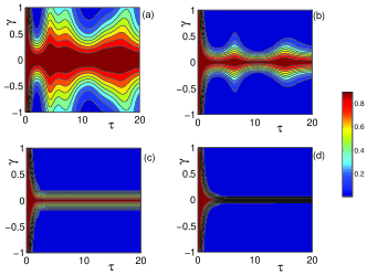
Figure 1: (color online) Hahn echo of the spin-$\frac{1}{2}$ particle vs. time $\tau$ and the anisotropy parameter $\gamma$. The spin-$\frac{1}{2}$ particle was coupled to a spin-chain described by the XY model. The parameters chosen are $N=246$ sites, $g=0.3$ and (a)$\lambda=2$, (b) $\lambda=1.5$, (c)$\lambda=1$, and (d)$\lambda=0.5$.

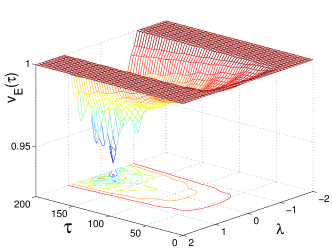
Figure 2: (color online)Hahn echo as a function of time $\tau$ and $\lambda$. The figure was plotted for $N=246$ sites, $g=0.1$ and $\gamma=0.001$.

We would like to notice that the Hahn echo $v_{E}(\tau)$ at critical points of $\gamma=0$ and $\lambda=\pm 1$ does not depend on the chain-system coupling constant $g$, but in the vicinity of $\gamma=0$, it does. This was shown in figure 3, where we plotted the Hahn echo as a function of $\lambda$ and $g$ with $\gamma=0.001$ (close to zero). As expected, the critical points have been shifted linearly by the coupling constant $g$. The white area in figure 3 corresponds to $v_{E}(\tau)=1$. In the region of $g>2$ and $-1<\lambda<1$, $v_{E}(\tau)$ always equal to 1. This can be understood by examining the the definition of $\theta_{j,k}$ and $\theta_{k}$. In this region, $\lambda_{j}=\lambda\pm g\geq 1$, leading to $\theta_{j,k}=\theta_{k}$ for any $k$ in the limit $\gamma\rightarrow 0$. This results in $v_{E}(\tau)=1$, which is a direct followup of Eq.(16).

Now we turn to study the criticality in the transverse Ising model($\gamma=1$ in the XY model). The ground state structure of this model change dramatically as the parameter $\gamma$ is varied. We first summarize the ground states of this model in the limits of $|\lambda|\rightarrow\infty$, $|\lambda|=1$ and $\lambda=0$. The ground state of the spin-chain approaches a product of spins pointing the positive/negative $z$ direction in the $|\lambda|\rightarrow\infty$ limit, whereas the ground state in the limit $\lambda=0$ is doubly degenerate under the global spin flip by $\prod_{l=1}^{N}\sigma_{l}^{z}$. At $|\lambda|=1$, a fundamental transition in the ground state occurs, the symmetry under the global spin flip breaks at this point and the chain develops a nonzero magnetization $\langle\sigma_{x}\rangle\neq 0$ which increases with $\lambda$ growing.

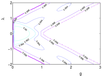
Figure 3: (color online)This figure was plotted to show the dependence of the critical points on the system-chain coupling constant $g$. Time $\tau=50$, $N=246$ sites, and $\gamma=0.001$ were chosen for this figure.

The above mentioned properties of the ground state are reflected in the Hahn echo as shown in figure 4. In the limit $|\lambda|\rightarrow\infty$, $\theta_{j,k}=\theta_{k}=\pi/(-\pi)$, this results in $v_{E}(\tau)=1$. In fact as figure 4-(a) shows, when $|\lambda|\geq 4$, $v_{E}(\tau)$ approaches 1 very well. With $|\lambda|\rightarrow 1$, the Hahn echo $v_{E}(\tau)$ tends to zero, this can be interpreted as the sensitivity of the spin-chain ground state to perturbations from the system-chain coupling at these points. The Hahn echo is a oscillating function of time $\tau$ around $\lambda=0$. Due to the coupling to the spin-chain, the oscillation is damping, and eventually $v_{E}(\tau)$ tends to zero in the $\tau\rightarrow\infty$ limit.

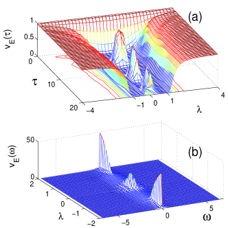
Figure 4: (color online)(a)Hahn echo versus time $\tau$ and $\lambda$ with $\gamma=1$. The other parameters chose are $g=0.1$, $N=246$ sites. (b) Discrete Fourier transformation of $v_{E}(\tau)$, with the same parameters as in figure (a).

The difference between cases of $\gamma=0$ and $\gamma=1$ is that $[n_{\uparrow,k},n_{\downarrow,k}]=0$ for $\gamma=0$, but it does not hold for $\gamma=1$. This is the reason why the Hahn echo takes different values at these critical points.Figure 4-(b) is a discrete Fourier transformation of $v_{E}(\tau)$ with the same parameters as in figure 4-(a). It would provides us the Hahn echo in the frequency domain. The ground state of the XY model is really complicated with many different regime of behaviorbarouch70 , these are reflected in sharp changes in the Hahn echo across the line $|\lambda|=1$ regardless of $\gamma$ (as shown in figure 5, except $\gamma=0$), indicating the change in the ground state of the spin-chain from paramagnetic phase to the others.

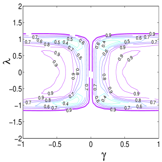
Figure 5: (color online)Hahn echo at time $\tau=20$ with $N=246$ sites, and $g=0.01$.

Up to now, we did not consider the temperature effect. Finite temperature is the regime to which all experiments being confined, but what is the finite temperature effect on the Hahn echo? In the following, we shall consider this problem by studying the contributions of one- and two-particle excitations to the Hahn echo. Taking a thermal state $\rho_{c}^{T}(0)=\frac{1}{z}e^{-\beta H_{c}}$ $(\beta=\frac{1}{k_{B}T}$) as the initial state of the spin-chain, the Hahn echo envelope can be written as

$$v_{E}^{T}(\tau)=\prod_{k}|1+\frac{1}{z}\sum_{n}e^{-\beta\Omega_{n}}\langle n|u_{\downarrow,k}^{\dagger}\hat{X}_{k}u_{\uparrow,k}|n\rangle|,$$ (17)

where $|n\rangle$ and $\Omega_{n}$ denote the eigenstate and corresponding eigenvalue of $H_{c}$, respectively. $z$ is the partition function.

Figure 6: (color online) Contribution of the two-particle excitation to Hahn echo at time $\tau=40$. The other parameters chosen are $N=246$ sites, $\gamma=0.01$, and $g=0.02$.

We shall restrict our consideration to the contribution from one- and two-particle excitations of the chain, namely,

$$|n\rangle\in\{\eta_{j,k}^{\dagger}|g(\gamma,\lambda)\rangle,\eta_{i,k_{1}}^{\dagger}\eta_{j,k_{2}}^{\dagger}|g(\gamma,\lambda)\rangle\},$$

$$\mbox{ for }k_{1}\neq k_{2},\mbox{\ or \ }i\neq j,$$ (18)

with $k$, $k_{1}$ and $k_{2}$ ranging from $-N/2$ to $N/2-1$. It is not difficult to show that there are no contribution from the one particle excitation, because $\hat{X}_{k}$ creates or annihilates two particles with $k$ and $-k$ jointly. The numerical results presented in figure 6 show the contribution of the two-particle excitation to the Hahn echo, we find that the quantum critical points can influence the Hahn echo at a finite temperature. For the parameters chosen in figure 6, the contribution form the thermal excitation is larger than that from quantum fluctuation when $\beta<72=\beta_{c}$. Here we have scaled out an overall energy scale denoted by $J$. $J$ may be taken to be of order $1000K$, that is the order for the antiferromagnetic exchange constant of the Heisenberg model. It yields $T_{c}\sim 14K$ corresponding to parameters chosen in figure 6. For the transverse Ising model $\gamma=1$, $\beta_{c}$ is of order $10$, we obtain $T_{c}\sim 100K$ in this situation with the other parameters being the same as in figure 6. Notice that the study here is based on the Hahn echo(a dynamical quantity), this would differ from the investigation based on thermodynamicskopp05 . We would like to notice that the discussion on the finite temperature effect was limited to very low temperatures, because only one- and two-quasiparticle excitations were included. Nevertheless, it is interesting because it also sheds light on the contribution to Hahn echo from the first excited states, which have the same energy as the ground state $\rho_{c}(0)$ of $H_{c}$ at critical points. The results presented in figure 6 show that those contributions tend to zero with $T\rightarrow 0$.

In conclusion, by discussing the Hahn spin echo in the spin-$\frac{1}{2}$ particle coupled to critical spin-chains, the relation between the Hahn echo and the critical points was established. The relation not only provides an efficient theoretical tool to study quantum phase transitions, but also proposes a method to measure the critical points in experiments. Up to two-particle excitations, we have also studied the influence of thermal fluctuation on the Hahn echo, it would shed light on the low temperature(with respect to the overall energy scale $J$) effects on the Hahn echo.

This work was supported by NCET of M.O.E, and NSF of China Project No. 10305002 and 60578014.

References

- (1) S. Sachdev, Quantum Phase Transition (Cambridge University Press, Cambridge, 1999).
- (2) E. L. Hahn, Phys. Rev. 80, 580(1950).
- (3) A. Osterloh, L. Amico, G. Falci, and R. Fazio, Nature 416, 608(2002).
- (4) G. Vidal, J. I. Latorre, E. Rico, and A. Kitaev. Phys. Rev. Lett. 90, 227902(2003).
- (5) L. A. Wu, M. S. Sarandy, and D. A. Lidar, Phys. Rev. Lett. 93, 250404(2004).
- (6) Y. Chen, P. Zanardi, Z. D. Wang, and F. C. Zhang, e-print: quant-ph/0407228.
- (7) S. J. Gu, G. S. Tian, and H. Q. Lin, e-print: quant-ph/0509070.
- (8) A. Carollo, and J. K. Pachos, Phys. Rev. Lett. 95, 157203(2005).
- (9) S. L. Zhu, Phys. Rev. Lett.96, 077206(2006).
- (10) A. Hamma, e-print: quant-ph/0602091.
- (11) W. M. Witzel, R. de Sousa, and S. Das Sarma, Phys. Rev. B 72, 161306(2005).
- (12) H. T. Quan, Z. Song, X. F. Liu, P. Zanardi, and C. P. Sun, e-print: quant-ph/0509007. To appear on Phys. Rev. Lett..
- (13) P. Zanardi, N. Paunkovic, e-print: quant-ph/0512249.
- (14) E. Barouch and B. M. McCoy, Phys. Rev. 2, 1075(1970); Phys. Rev. A 3, 786(1971).
- (15) A. Kopp, S. Chakravarty, Nature Physics 1, 53(2005).