Parity law of the singlet-triplet gap in graphitic ribbons

Abstract

This work explores the possibility to transfer the parity law of the singlet-triplet gap established for square ladders (gapped for even number of legs, gapless for odd number of legs) to fused polyacenic 1-D systems, i.e., graphite ribbons. Qualitative arguments are presented in favor of a gapped character when the number $n_{\omega}$ of benzene rings along the ribbon width is odd. A series of numerical calculations (quantitative mapping on spin $1/2$ chains, renormalized excitonic treatments and Quantum Monte Carlo) confirm the parity law and the gapless character of the ribbon for even $n_{\omega}$.

1 Introduction

In the recent past the properties of some quasi 1-D strongly correlated materials, namely cuprate ladders, have attracted much interest from solid state physicists Dagotto . As a major result they have established that the spin gap (i.e., lowest singlet to triplet excitation energy) of spin $1/2$ ladders presents a parity law: the ladders are gapped (have a finite excitation energy) when the number of legs is even, and gapless (degenerate singlet and triplet state) for odd number of legs Ref1 . This result was not expected, since one may consider the ladders as intermediate between the simple 1-D chain and the square 2-D lattice, which are both gapless.

Finite ribbons of fused polyacenes (with CH bonds on the most external doubly-bonded carbons) can be seen as organic analogs of the cuprate ladders. They are quasi 1-D fragments of graphite, which is gapless. The non-dimerized linear polyene is also known to be gapless. In light of the recent investigations on both carbon and spin nanotubes, we can extend the discussion on the link between magnetic properties and geometry of such objects Matsumoto . In particular, are the fused polybenzenoïd ribbons always gapless ?

Although the $\pi$-electrons of the conjugated hydrocarbons are not strongly correlated, it has been shown twenty years ago that they can be treated accurately through $S=1/2$ Heisenberg Hamiltonians

$$H=J\sum_{\left<i,j\right>}{\bf S}_{i}\cdot{\bf S}_{j}$$ (1)

i.e., as spins interacting with their nearest neighbours through antiferromagnetic (AF) couplings $J>0$ Ref2 ; Ref3 . This effective model is not based on the usual perturbative approach in the strong coupling limit; instead the amplitude of the exchange integral is given by the exact solution of the 2-site problem. More explicitely, for a Hubbard Hamiltonian, the AF coupling is no longer taken as its perturbative estimate $J=4t^{2}/U$, but rather as the exact energy difference between the triplet and singlet states $J=-(U-\sqrt{U^{2}+16t^{2}})/2.$ This view of $\pi$-electron systems offers simple rationalizations of many of their properties. In particular, a geometry-dependent Heisenberg Hamiltonian (with $J(r)$ depending on the distance $r$ between sites) has been extracted from accurate calculations of the singlet and triplet states of ethylene and happens to be a quantitative tool for the ground and lowest excited states of conjugated hydrocarbons Ref2 ; Ref3 (a spin-independent $V(r)$ potential is of course also needed in that case to take into account the $r$-dependences of the localized $\sigma$-bonds). This analysis was proved in various situations to be very predictive: for instance, the ground-state geometries of a large series of hydrocarbones are accurately reproduced by minimizing the lowest eigenvalue of the geometry-dependent Hamiltonian with respect to the bond distance Ref2 . It was also shown that the vertical excitation spectrum to the lowest triplet states is in good agreement with experiments Ref3 and that the excited state geometries and vertical emission energies Ref3 agree with accurate ab initio calculations. This magnetic model has been widely and successfully used by Robb et al. Ref4 under the acronym MM-VB (Molecular Mechanics Valence Bond) for the study of the photochemistry of conjugated hydrocarbons.

Figure 1: Two-leg ladder (A) and $n_{\omega}=1$ fused polyacene (B), and their mapping into dimerized spin 1/2 chains. In this figure and the following ones, the symbols $\circ$ and $*$ correspond to up and down spins respectively; the resulting effective models appear just below each lattice. We denote with a single- and double-line the effective couplings when they are different. For the graphitic ribbons, dotted lines separate the different blocks used in the calculation (see text).

In fact, it is quite natural to expect, at least for bipartite lattices, the lowest excitation energies to be correctly described by a (properly normalized) Heisenberg Hamiltonian as the lowest states are dominated by neutral VB configurations and as the antisymmetrization favours an antiferromagnetic order independently of the value of $U$ Lepetit89 . Of course, the charge excitations, essentially leading to ionic states, are not accessible with these approaches, but it is known for idealized 1D chains lieb and from experiments on conjugated molecules hudson that the dipolarly-allowed VB ionic states are located at higher energies than the lowest triplet (and even than neutral singlet states).

We now only consider the purely magnetic model of Eq. (1). A few years ago density matrix renormalization group (DMRG) calculations have been reported, concerning the singlet-triplet gap of the simplest polyacenic chain, built of aligned fused benzene rings Ref5 . The extrapolated calculated gap is finite and close to $0.1J$. Actually the polyacene can be viewed as a two-leg ladder in which one rung over two has vanished (see Fig. 1). One might wonder whether there is a similarity between the three-leg ladder and a fused polyacenic infinite ribbon with two ranks of benzene rings (see Fig. 3). From qualitative arguments one may conjecture that the singlet-triplet excitation in such polyacenic ribbons of graphite is finite when the number of superposed rings in the width of the ribbon, $n_{\omega}$, is odd and vanishes when $n_{\omega}$ is even. Numerical calculations using the quantitative mapping on known 1-D chains, renormalized excitonic method (REM) Ref5bis , and Quantum Monte Carlo calculations (QMC), show that the gap indeed vanishes for even $n_{\omega}$ and is non-zero for odd $n_{\omega}$ ribbons.

2 Qualitative arguments

Qualitative arguments can be used to rationalize the parity law of ladders, which can also be applied to 1-D fused polyacenes. They are based on the real-space renormalization group (RSRG), originally proposed by Wilson Ref6 . Concerning spin lattices one may consider that they are built from blocks rather than from sites. Of course these blocks interact. If the blocks do not have a singlet ground state, but a doublet, or a triplet, they can be seen as interacting effective spins Ref7 . A quasi 1-D lattice can then be easily transformed Ref8 into a simple 1-D spin chain, the properties of which are well known. Considering 2-leg ladders, one may define $(2N_{s}+1)$ sites blocks, which have a ground state doublet $(S_{z}=\pm 1/2)$. But these blocks do not have equal interactions with their left and right nearest neighbors (cf. figure 1 (A)). Consequently, the 2-leg ladder maps into a dimerized (i.e., bond-alternated) spin $1/2$ chain, which is known to be gapped. An alternative partition uses blocks with even number of sites (figure 2 (A)) which have a triplet ground-state. The resulting effective $S=1$ chain exhibits the famous Haldane gap Ref9 and therefore both partitions predict a gap.

Figure 2: Mapping of ladder and polyacene into a spin-1 chain.

If one applies the same arguments to the $n_{\omega}=1$ polyacenic chain one obtains a similar mapping pictured in figure 1 (B). The partition into blocks of $(4N_{S}+1)$ sites and $(4N_{S}+3)$ sites produces an alternating dimerized spin chain, which is gapped. The partition into $4N_{S}$ sites blocks with triplet ground states (figure 2) leads to a Haldane gap Ref9 . Both partitions suggest a finite excitation energy.

The ladder with odd number of legs can be partitioned into blocks with odd number of sites which have equal interactions with the left and right neighbors, and the ladders can be mapped into a non-dimerized gapless 1-D $S=1/2$ chain, (cf. figure 3 (A)). For the $n_{\omega}=2$ polybenzenoïd ribbon the simplest partition defines 9-site blocks presenting a $S=1/2$ ground state and equal AF interactions with left and right nearest neighbors (cf. Fig. 3 (B)). The resulting mapping to an effective AF uniform chain indicates that the $n_{\omega}=2$ polyacenic ribbon should not be gapped. This is actually one of the two possibilities allowed by the famous Lieb-Schultz-Mattis theorem LSM which can be applied for even $n_{\omega}$ (where the unit cell contains an odd number of spin $1/2$). If even $n_{\omega}$ lattices do have a gap, this theorem guarantees that the system breaks translation symmetry.

Figure 3: Three-leg ladder (A) and $n_{\omega}=2$ fused polyacene (B), and their mapping into spin 1/2 chains.

The arguments can easily be generalized to any thickness of the ribbon according to figure 4, which proposes a mapping into an uniform $S=1/2$ spin chain for even values of $n_{\omega}$ and into an uniform integer-spin $S$ chain for odd $n_{\omega}$. Of course the $S=1$ chain may be transformed into a dimerized chain of $S=1/2$ blocks by shifting one external carbon from one block to its right side neighbor block.

Figure 4: Generalization of the mappings on non-dimerized AF $S=1/2$ chains for even $n_{\omega}$ (A) and $S=1$ chains for odd $n_{\omega}$ (B). Moving the $(\ast)$ atom to the right-side block leads to an effective dimerized $S=1/2$ AF chains.

3 Numerical studies

We now turn to numerical verifications of that conjecture for $n_{\omega}=1,2$ and 3 with several different techniques. Note that DMRG calculations have already been performed for the $n_{\omega}=1$ case Ref5 . For larger $n_{\omega}$, the number of states to be kept becomes too large and the computation cost is prohibitive. Therefore, after providing quantitative estimates for the spin gap using approximate techniques, we have adressed this issues by using an efficient QMC method.

3.1 Mapping into 1-D chains

For $n_{\omega}=1$ the chain may be considered as built from $A$ and $B$ blocks of 7 and 9, 9 and 11, 11 and 13, or 13 and 15 sites, according to figure 1 (B). One then obtains a dimerized $S=1/2$ spin chain with different values $J_{1}$, $J_{2}$ between the $A-B$ and $B-A$ blocks. The effective interactions $J_{1}$ and $J_{2}$ are directly obtained from the energy difference between the lowest triplet and singlet energies of $A-B$ and $B-A$ blocks :

Blocks	7-9	9-11	11-13	13-15
$J_{1}$	0.221	0.196	0.181	0.170
$J_{2}$	0.166	0.123	0.095	0.075

A previons study of the dimerized $S=1/2$ chain has suggested that the gap follows the law Ref7  :

$$\Delta E=(J_{1}+J_{2})\delta^{0.71}\ \mbox{with}\ \delta=\frac{(J_{1}-J_{2})}{(J_{1}+J_{2})}.$$ (2)

Applying Eq. (2) one obtains

$$\Delta E = 0.097J\ \mbox{for the (7-9) blocks},$$

$$\Delta E = 0.112J\ \mbox{for the (9-11) blocks},$$

$$\Delta E = 0.121J\ \mbox{for the (11-13) blocks},$$

$$\Delta E = 0.126J\ \mbox{for the (13-15) blocks},$$

hence a finite gap.

For $n_{\omega}=2$ the simple mapping into a non-dimerized $S=1/2$ AF spin chain of 9-site blocks (cf. figure 3 (B)) pleads in favor of a gapless character, but this construction assumes only nearest-neighbor effective interaction $J_{NN}$, neglecting for instance next-nearest neighbors interactions $J_{NNN}$. In fact, an uniform AF chain becomes gapped when the ratio $J_{NNN}/J_{NN}$ is larger than 0.241 Ref10 . We have extracted the effective couplings between 9-site blocks (figure 3 (B)) from the exact spectrum of the trimer of blocks and we found an AF coupling between $NN$ blocks $J_{NN}=0.15896$ (in good agreement with the value extracted from the dimer $J_{NN}=0.16622$) and a surprisingly large ferromagnetic $J^{\prime}_{NNN}=-0.1705$ coupling. Since an AF $S=1/2$ chain with ferromagnetic coupling between $NNN$ sites is not gapped, the $n_{\omega}=2$ ribbon should be gapless.

For $n_{\omega}=3$ one may define a dimerized AF $S=1/2$ chain of 13 and 11 sites respectively as pictured in figure 5. One obtains two values of the inter block AF coupling ($J_{1}=0.115$, $J_{2}=0.108$). Using equation (2) one obtains $\Delta E(n_{\omega}=3)=0.018J$.

Figure 5: Definition of the blocks for a mapping into a dimerized $S=1/2$ chain of $n_{\omega}=3$ ribbon.

3.2 Renormalized excitonic calculations

The recently proposed renormalized excitonic method Ref5bis is again based on a periodic partition into blocks, but now the blocks have an even number of sites, a singlet ground state $\psi_{A}^{0}$ and a triplet lowest excited state $\psi_{A}^{\ast}$. One defines a model space for the $AB$ dimers made of two adjacent blocks, spanned by local singly excited states $\psi_{A}^{\ast}\psi_{B}^{0}$ and $\psi_{A}^{0}\psi_{B}^{\ast}$. Knowing the spectrum of the $AB$ dimer, it is possible to define Ref11

• the effective energy of $\psi_{A}^{\ast}\psi_{B}^{0}$ and $\psi_{A}^{0}\psi_{B}^{\ast}$,

• the effective interaction between them.

These informations allow to apply the excitonic method. For the infinite lattice, this method leads to the following expressions of the excitation energy

$$\Delta E^{\infty}(N_{S})=2\Delta E(2N_{S})-\Delta E(N_{S}).$$ (3)

obtained from the gap values for a $N_{S}$-site block ($\Delta E(N_{S})$) and for a dimer ($\Delta E(2N_{S})$).

Figure 6: Definition of blocks for the calculation of the energy gap through the REM.

The method has been applied with success to the 2-leg ladders Ref8 and can be applied to $n_{\omega}=1$, $n_{\omega}=2$ and $n_{\omega}=3$ polybenzenoïd ribbons using the design of the blocks pictured in figure 6.

We find a finite gap for $n_{\omega}=1$ polyacene:

$$\Delta E^{\infty}(8) = 0.068J\ \mbox{for}\ N_{S}=8\ \mbox{sites blocks,}$$

$$\Delta E^{\infty}(12) = 0.094J\ \mbox{for}\ N_{S}=12\ \mbox{sites blocks.}$$

Since the $N_{S}^{-1}$ components of the excitation energy cancels in the expression of $\Delta E^{\infty}(N_{S})$, an extrapolation in terms of $N_{S}^{-2}$ leads to $\Delta E(n_{\omega}=1)=0.103J$.

The result of the REM method for the $n_{\omega}=2$ lattice from the $N_{S}=12$ sites blocks is one order of magnitude smaller, $\Delta E^{\infty}(12)=0.013J$. Extrapolation is not possible in this problem, but this result supports the conjecture that this fused polybenzenoïd ribbon is not gapped.

For $n_{\omega}=3$ unequal blocks of $N_{S}=14$ and $N_{S}=10$ sites have been used, according to figure 6. Since the blocks are different it is necessary to generalize the algebra of Ref. 6, as performed in the Appendix. The final result is $\Delta E^{\infty}(14,10)=0.0125J$. Even if the results for the gaps for $n_{\omega}=2$ and $3$ are quite close, these calculations support the idea of a constrast between the odd and even ribbons. In order to confirm this conjecture, we now present accurate Quantum Monte Carlo results for the $n_{w}=1,2$ and $3$ ribbons.

3.3 Quantum Monte Carlo

As the spin lattices are not frustrated, efficient QMC algorithms are available which allow to simulate with high-precision large systems at finite, albeit extremely small, temperatures. Here we use a multi-cluster continuous time beard loop algorithm evertz which is free of any systematic errors. We simulate systems of sizes up to length $L=800$ (the total number of spins is $N=2(n_{\omega}+1)L$) and at inverse temperature up to $\beta J=J/T=1000$. We use periodic boundary conditions along the legs. To determine the gapfull/gapless nature of the systems, we calculate the correlation length in imaginary time $\xi_{\tau}$ with the help of a standard second moment estimator cooper ; todo

$$\xi_{\tau}=\frac{\beta}{2\pi}\left(\frac{\chi(\omega=0)}{\chi(\omega=2\pi/\beta)}-1\right)^{1/2}$$ (4)

where $\chi(\omega)=\int_{0}^{\beta}d\tau e^{i\omega\tau}\chi(\tau)$ is the Fourier-transform of the imaginary time dynamical antiferromagnetic structure factor $\chi(\tau)=\frac{1}{\beta N}\sum_{i,j}(-)^{r_{j}-r_{i}}\int_{O}^{\beta}dtS^{z}_{i}(t)S^{z}_{j}(t+\tau)$. It can be shown that for a gapped system, $\xi_{\tau}$ converges to the inverse spin gap in the thermodynamic limit at zero temperature : $\lim_{L,\beta\rightarrow\infty}\xi_{\tau}(L,\beta)=(\Delta E)^{-1}$. On the other hand, when the system is gapless, $\xi_{\tau}^{-1}$ is an upper bound of the finite-size gap for any finite $L$ and $\beta$. In fig. 7, we represent the inverse of the imaginary correlation length $(J\xi_{\tau})^{-1}$ as a function of the temperature $T/J$ in log-log scale, for the three types of ribbons $n_{\omega}=1,2$ and $3$. This representation is useful to see if the system is gapped as $(J\xi_{\tau})^{-1}$ saturates at low temperatures to the gap value $\Delta E/J$.

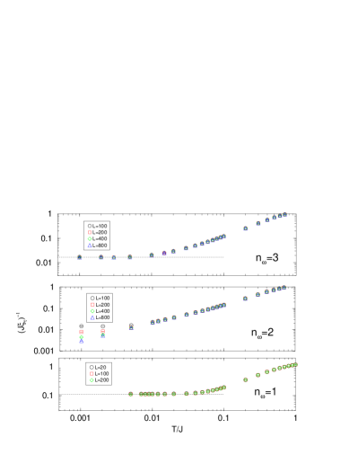
Figure 7: Quantum Monte Carlo results for the inverse of the imaginary time correlation length as a function of temperature for the $n_{\omega}=1$ (bottom panel), $n_{\omega}=2$ (middle panel) and $n_{\omega}=3$ (top panel), for different system sizes $L$. Values of the extracted gaps $\Delta E(n_{\omega}=1)=0.1112(7)J$ and $\Delta E(n_{\omega}=3)=0.0164(4)J$ are represented by dashed-lines for $n_{\omega}=1$ and $3$.

For $n_{\omega}=1$, $(J\xi_{\tau})^{-1}$ clearly converges at low $T$ to a minimum value identical for system sizes $L=100$ and $L=200$, indicating that finite-size effects are absent. From the results for the largest $L$ at the lowest $T$, we extract the value of the spin gap $\Delta E(n_{\omega}=1)=0.1112(7)J$, in perfect agreement with DMRG calculations Ref5 .

We find no saturation of $(J\xi_{\tau})^{-1}$ at the lowest temperature for the largest system size $L=800$ studied for $n_{\omega}=2$. Data for smaller systems ($L=100,200$) present signs of saturation at low enough $T$ towards values which depend on the system size: this is naturally interpreted as the signature of finite-size gaps. Strictly speaking, the numerical data for the largest $L$ at the lowest $T=0.001$ can only put an upper bound $\Delta E(n_{\omega}=2)<0.0030J$ on the value of the gap. However, the general form of the $T$ dependence of $(J\xi_{\tau})^{-1}$ and the fact that we still have finite-size effects for large systems at low $T$ naturally indicate that the $n_{\omega}=2$ system is gapless, i.e. $\Delta E(n_{\omega}=2)=0$.

Finally for $n_{\omega}=3$, a convergence of $(J\xi_{\tau})^{-1}$ is recovered at low enough $T$ towards a size-independent constant. As for the $n_{\omega}=1$ case, this indicates that the system is gapped and we obtain the gap value $\Delta E(n_{\omega}=3)=0.0164(4)J$. Please note that we had to resort to large systems at very low temperatures ($L=800$ and $T=0.001$) to assert the complete convergence of our data: this is ascribed to the small value of the gap (an order of magnitude lower than for $n_{\omega}=1$).

In conclusion, the QMC simulations unambiguously proove the even/odd number $n_{\omega}$ effect for the gapless/gapfull nature of 1-D fused polyacenic ribbons. As for spin ladders, we find that the value of the gap decreases with the number $n_{\omega}$ of rings along the width for odd $n_{\omega}$ ribbons.

4 Conclusion

The conjecture of the existence of parity law concerning the spin gap in polybenzenoïd ribbons (vanishing / finite gap for even / odd $n_{\omega}$) was proposed on the ground of qualitative arguments. This conjecture is confirmed by a consistent set of numerical calculations summarized in table 1.The REM fails to give a zero gap for $n_{\omega}=2$ but indicates a contrast between odd and even ribbons. The quantitative mapping and the accurate QMC calculations confirm the gapless character of the $n_{\omega}=2$ ribbons and agree on the amplitude of the gap for $n_{\omega}=1$ and $n_{\omega}=3$. For graphite ribbons Ref2 ; Ref3 , for which $J\sim 2.2$ eV at the typical $r_{cc}$ distance (1.395Å), the gaps should be close to $0.23$ eV for $n_{\omega}=1$ and $0.03$ eV for $n_{\omega}=3$. Despite the semi-metallic nature of graphite, it seems unlikely that the odd-$n_{\omega}$ ribbons present a zero charge gap, below their finite spin-gap. We finally note, in analogy with the study of the influence of four-spin operators in spin ladders 4spin , that it would be worth considering the possible impact of six-spin operators on such graphitic ribbons since their amplitude is not negligible in hexagons Maynau1 ; Maynau2 .

	Mapping	REM	QMC
$n_{\omega}=1$	0.126	0.103	0.1112(7)
$n_{\omega}=2$	0	0.013	0
$n_{\omega}=3$	0.018	0.0125	0.0164(4)

Table 1: Calculed gaps (in units of $J$) obtained from different methods.

5 Acknowledgments

The QMC calculations were performed using the looper application todo (see http://wistaria.comp-phys.org/alps-looper ) of the ALPS library ALPS (see http://alps.comp-phys.org). We warmly thank A. Läuchli for suggesting the LSM argument for even $n_{\omega}$.

Appendix A Renormalized excitonic method for an $(A-B)_{n}$ chain

One has two types of blocks $A$ and $B$. The ground state and lowest excited eigenfunctions for each block are given by

$$H_{A}|\psi^{0}_{A}\rangle = E^{0}_{A}|\psi^{0}_{A}\rangle,$$

$$H_{A}|\psi_{A}^{\ast}\rangle = E^{\ast}_{A}|\psi_{A}^{\ast}\rangle,$$

$$H_{B}|\psi^{0}_{B}\rangle = E^{0}_{B}|\psi^{0}_{B}\rangle,$$

$$H_{B}|\psi_{B}^{\ast}\rangle = E^{\ast}_{B}|\psi_{B}^{\ast}\rangle.$$

The ground state of the chain is represented by

$$\Psi^{0}=\prod_{i}\psi^{0}_{A_{i}}\prod_{j}\psi^{0}_{B_{j}}.$$

Its energy will be

$$\langle\Psi^{0}|H^{eff}|\Psi^{0}\rangle=n(E^{0}_{A}+E^{0}_{B})+n(v_{AB}+v_{BA}).$$

The interaction energies between two adjacent blocks is given by the knowledge of the exact energies of the $AB$ and $BA$ dimers

$$H_{AB}|\Psi^{0}_{AB}\rangle=E^{0}_{AB}|\Psi^{0}_{AB}\rangle,\ E^{0}_{AB}=E^{0}_{A}+E^{0}_{B}+v_{AB}.$$

For the description of excited states one needs to estimate the effective interaction between a local excited state and the neighbor ground states and the integral responsible for the transfer of excitation. These informations are obtained from the excited solutions of the dimers. One should especially consider the two eigenstates

$$H_{AB}|\Psi_{AB}^{\ast}\rangle = E^{\ast}_{AB}|\Psi_{AB}^{\ast}\rangle,$$

$$H_{AB}|\Psi_{AB}^{\ast^{\prime}}\rangle = E^{\ast^{\prime}}_{AB}|\Psi_{AB}^{\ast^{\prime}}\rangle,$$

having the largest projections $|\tilde{\Psi}_{AB}^{\ast}\rangle$ and $|\tilde{\Psi}_{AB}^{\ast^{\prime}}\rangle$, on the model space spanned by $\psi_{A}^{\ast}\psi_{B}^{0}$ and $\psi_{A}^{0}\psi_{B}^{\ast}$, which can be written after orthogonalization as

$$|\tilde{\Psi}_{AB}^{\ast}\rangle = \lambda|\psi_{A}^{\ast}\psi_{B}^{0}\rangle+\mu|\psi_{A}^{0}\psi_{B}^{\ast}\rangle,$$

$$|\tilde{\Psi}_{AB}^{\ast^{\prime}}\rangle = -\mu|\psi_{A}^{\ast}\psi_{B}^{0}\rangle+\lambda|\psi_{A}^{0}\psi_{B}^{\ast}\rangle.$$

It results that

$$\langle\psi_{A}^{\ast}\psi_{B}^{0}|H^{eff}|\psi_{A}^{\ast}\psi_{B}^{0}\rangle = \lambda^{2}E^{\ast}_{AB}+\mu^{2}E^{\ast^{\prime}}_{AB}$$

$$= E^{\ast}_{A}+E^{0}_{B}+v_{(A^{\ast})B},$$

$$\langle\psi_{A}^{0}\psi_{B}^{\ast}|H^{eff}|\psi_{A}^{0}\psi_{B}^{\ast}\rangle = \mu^{2}E^{\ast}_{AB}+\lambda^{2}E^{\ast^{\prime}}_{AB}$$

$$= E^{0}_{A}+E^{\ast}_{B}+v_{A(B^{\ast})},$$

$$\langle\psi_{A}^{\ast}\psi_{B}^{0}|H^{eff}|\psi_{A}^{0}\psi_{B}^{\ast}\rangle = (E^{\ast}_{AB}-E^{\ast^{\prime}}_{AB})\lambda\mu=h_{AB}.$$

For the periodic system the delocalized excited states will be respresented as linear combinations of locally excited states on either $A$ or $B$ blocks

$$\Psi^{\ast}_{A_{m}} = \psi^{\ast}_{A_{m}}\prod_{i\neq m}\psi^{0}_{A_{i}}\prod_{j}\psi^{0}_{B_{j}},$$

$$\Psi^{\ast}_{B_{n}} = \psi^{\ast}_{B_{n}}\prod_{j\neq n}\psi^{0}_{B_{j}}\prod_{i}\psi^{0}_{A_{i}},$$

The energies of $\Psi^{\ast}_{A_{m}}$ and $\Psi^{\ast}_{B_{n}}$ are given by

$$\langle\Psi^{\ast}_{A_{m}}|H^{eff}|\Psi^{\ast}_{A_{m}}\rangle-\langle\Psi^{0}|H^{eff}|\Psi^{0}\rangle=$$

$$E^{\ast}_{A}-E^{0}_{A}+v_{(A^{\ast})B}-v_{AB},$$

$$\langle\Psi^{\ast}_{B_{n}}|H^{eff}|\Psi^{\ast}_{B_{n}}\rangle-\langle\Psi^{0}|H^{eff}|\Psi^{0}\rangle=$$

$$E^{\ast}_{B}-E^{0}_{B}+v_{(B^{\ast})A}-v_{BA},$$

This locally excited state are coupled with the states locally excited on the adjacent $B$ blocks

$$\langle\Psi^{\ast}_{A_{m}}|H^{eff}|\Psi^{\ast}_{B_{m}}\rangle=h_{AB}.$$

For the lowest state of the lattice, corresponding to $\overrightarrow{k}=0$, the delocalized excited states can be written as a linear combination of

$$(\Psi^{\ast}_{a})_{\overrightarrow{k}=0}=\frac{1}{\sqrt{N}}\sum_{A_{m}}\Psi^{\ast}_{A_{m}},$$

and

$$(\Psi^{\ast}_{b})_{\overrightarrow{k}=0}=\frac{1}{\sqrt{N}}\sum_{B_{n}}\Psi^{\ast}_{B_{n}},$$

solution of a $2\times 2$ matrix whose elements are

$$\Big{\langle}(\Psi^{\ast}_{a})_{\overrightarrow{k}=0}\Big{|}H^{eff}\Big{|}(\Psi^{\ast}_{a})_{\overrightarrow{k}=0}\Big{\rangle}-\Big{\langle}\Psi^{0}\Big{|}H^{eff}\Big{|}\Psi^{0}\Big{\rangle}=$$

$$E^{\ast}_{A}-E^{0}_{A}+2\Big{(}V_{(A^{\ast})B}-V_{AB}\Big{)},$$

$$\Big{\langle}(\Psi^{\ast}_{b})_{\overrightarrow{k}=0}\Big{|}H^{eff}\Big{|}(\Psi^{\ast}_{b})_{\overrightarrow{k}=0}\Big{\rangle}-\Big{\langle}\Psi^{0}\Big{|}H^{eff}\Big{|}\Psi^{0}\Big{\rangle}=$$

$$E^{\ast}_{B}-E^{0}_{B}+2\Big{(}V_{(B^{\ast})A}-V_{BA}\Big{)},$$

$$\Big{\langle}(\Psi^{\ast}_{a})_{\overrightarrow{k}=0}\Big{|}H^{eff}\Big{|}(\Psi^{\ast}_{b})_{\overrightarrow{k}=0}\Big{\rangle}=2h_{AB}.$$

References

- (1) E. Dagotto and T.M. Rice, Science 271, 618 (1996).
- (2) S. R. White, R.M. Noack, and D. J. Scalapino, Phys. Rev. Lett. 73, 886 (1994).
- (3) See M. Matsumoto et al., Physica E 29, 660 (2005) and references therein.
- (4) M. Said, D. Maynau, J.-P. Malrieu, and M. A. G. Bach, J. Am. Chem. Soc. 106, 571 (1984).
- (5) M. Said, D. Maynau, and J.-P. Malrieu, J. Am. Chem. Soc. 106, 580 (1984).
- (6) F. Jolibois, M. J. Bearpark, S. Klein, M. Olivucci, and M. A. Robb, J. Am. Chem. Soc. 122, 5801 (2000).
- (7) M.-B. Lepetit, B. Oujia, J.-P. Malrieu, and D. Maynau, Phys. Rev. A 39, 3274 (1989).
- (8) E.H. Lieb and F.Y. Wu, Phys. Rev. Lett. 20, 1445 (1968)
- (9) B.S. Hudson, B.E. Kohler and K. Schulten, in Excited states Vol. 6, E.C. Lin ed. (Academic, New York, 1982)
- (10) Y. Gao, C.-G. Liu, and Y.-S. Jiang, J. Phys. Chem. A 106, 2592 (2002).
- (11) M. Al Hajj, J.-P. Malrieu, and N. Guihéry, Phys. Rev. B 72, 224412 (2005).
- (12) K.G Wilson, Rev. Mod. Phys. 47, 773 (1975).
- (13) J.-P. Malrieu and N. Guihéry, Phys. Rev. B 63, 085110 (2001).
- (14) M. Al Hajj, N. Guihéry, J.-P. Malrieu, and B. Bocquillon, Eur. Phys. J. B 41, 11 (2004).
- (15) F. D. M. Haldane, Phys. Lett. A 93, 464 (1983).
- (16) E. Lieb, T. Schultz, and D. Mattis, Ann. Phys. (N.Y.) 16, 407 (1961).
- (17) S. Eggert, Phys. Rev. B 54, 9612 (1996).
- (18) C. Bloch, Nucl. Phys. 6, 329 (1958).
- (19) B.B. Beard and U.-J. Wiese, Phys. Rev. Lett. 77, 5130 (1996).
- (20) H.G. Evertz, G. Lana and M. Marcu, Phys. Rev. Lett. 70, 875 (1993).
- (21) F. Cooper, B. Freedman and D. Preston, Nucl. Phys. B 210, 210 (1982).
- (22) S. Todo and K. Kato, Phys. Rev. Lett. 87, 047203 (2001).
- (23) See e.g. A. Läuchli, G. Schmid and M. Troyer, Phys. Rev. B. 67, 100409(R) (2003), and references therein.
- (24) D. Maynau, P. Durand, J.-P. Daudey and J.-P. Malrieu, Phys. Rev. A 28, 3190 (1983)
- (25) D. Maynau and J.-P. Malrieu, J. Am. Chem. Soc. 104, 3021 (1982).
- (26) F. Alet et al., J. Phys. Soc. Jap. Suppl. 74, 30 (2005); M. Troyer, B. Ammon and E. Heeb, Lect. Notes Comput. Sci., 1505, 191 (1998).