Band Engineering in Cooper-Pair Box: Dispersive Measurements of Charge and Phase

Abstract

Low-frequency susceptibility of the split Cooper-pair box (SCPB) is investigated for use in sensitive measurements of external phase or charge. Depending on the coupling scheme, the box appears as either inductive or capacitive reactance which depends on external phase and charge. While coupling to the source-drain phase, we review how the SCPB looks like a tunable inductance, which property we used to build a novel radio-frequency electrometer. In the dual mode of operation, that is, while observed at the gate input, the SCPB looks like a capacitance. We concentrate on discussing the latter scheme, and we show how to do studies of fast phase fluctuations at a sensitivity of 1 mrad/$\sqrt{\mathrm{Hz}}$ by measuring the input capacitance of the box.

1 Introduction

Josephson junctions (JJ) store energy according to $E=-E_{J}\cos(\varphi)$, where $\varphi$ is the phase difference across the junction, and the Josephson energy $E_{J}$ is related to the junction critical current $I_{C}$ through $I_{C}=2eE_{J}/\hbar$. Since JJ’s also typically exhibit negligible dissipation, they can be used as reactive circuit components. By combining the Josephson equations $I=I_{C}\sin(\varphi)$ and $\dot{\varphi}=2eV(t)/\hbar$, where $V(t)$ is the voltage across the junction, we find that a single JJ behaves as a nonlinear inductance,

$$L_{J}(\varphi)=\frac{\hbar}{2eI_{C}\cos(\varphi)}=\frac{L_{J0}}{\cos(\varphi)},$$ (1)

where we defined the linear-regime Josephson inductance $L_{J0}=\hbar/(2eI_{C})$.

Quantum effects in mesoscopic JJ’s widom84 ; Likharev85 may modify Eq. (1) in an important manner. In particular, the Josephson reactance may become capacitive AverinBruder03 ; Leif05 . In this brief communication, we investigate the Josephson reactance in the split Cooper-pair box (SCPB) geometry, with emphasis on detector applications. We first review the inductive susceptibility, and then concentrate on discussing the capacitive susceptibility in the spirit of a novel phase detector. The discussion relies heavily on the energy bands lukens $E_{k}$ of the SCPB, two lowest of them given in the limit $E_{J}/E_{C}\ll 1$ as

$$\begin{split}E_{0,1}&=E_{C}(n_{g}^{2}-2n_{g}+2)\mp\\ &\sqrt{\left(E_{J}\cos(\varphi/2)\right)^{2}+\left(2E_{C}(1-n_{g})\right)^{2}}-C_{g}V_{g}^{2}/2\end{split}$$ (2)

as a function of the classical fields $\varphi=2\pi\Phi/\Phi_{0}$ and $n_{g}=C_{g}V_{g}/e$ (see Fig. 1).

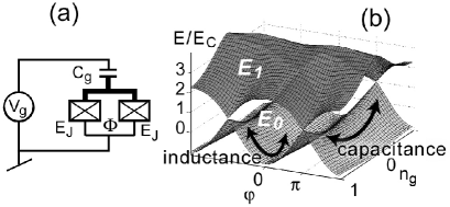
Figure 1: (a) Schematics of the SCPB. The mesoscopic island (thick line) has a total capacitance $C_{\Sigma}$ and charging energy $E_{C}=e^{2}/(2C_{\Sigma})$; (b) two lowest energy bands $E_{k}$ ($k=0,1$) of the SCPB , for $E_{J}/E_{C}=1.7$ (without the parabolic background $-(n_{g}e)^{2}/(2C_{g})$, see Eq. (2)). Inductive and capacitive susceptibilities are illustrated by the arrows parallel to $\varphi$ and $n_{g}$, respectively.

2 Quantum inductance

With respect to $\varphi$, the SCPT behaves as an inductance (Fig. 2 (b)), dependent, first of all, on the band index $k$, as well as on $n_{g}$ and $\varphi$:

$$L_{\mathrm{eff}}^{k}(n_{g},\varphi)=\left(\frac{d^{2}E_{k}}{d\Phi^{2}}\right)^{-1}=\left(\frac{\Phi_{0}}{2\pi}\right)^{2}\left(\frac{d^{2}E_{k}}{d\varphi^{2}}\right)^{-1}.$$ (3)

The strong $n_{g}$ dependence of $L_{\mathrm{eff}}^{0}$ when $E_{J}/E_{C}\ll 1$ has been used by the present authors to implement a fast reactive electrometer lset , using the scheme of Fig. 2 (a). The measurements are performed by studying the phase shift $\Theta=\arg(V_{\mathrm{out}}/V_{\mathrm{in}})$ of the ”carrier” microwave reflected from a resonant circuit containing the SCPB. Denoting by $Z$ the lumped-element impedance seen when looking towards the resonance circuit from the transmission line of impedance $Z_{0}=50\,\Omega$, the reflection coefficient of a voltage wave is

$$\Gamma=\frac{V_{\mathrm{out}}}{V_{\mathrm{in}}}=\frac{Z-Z_{0}}{Z+Z_{0}}=\Gamma_{0}e^{i\Theta}.$$ (4)

Since the whole setup consists in principle only of reactances, the inductively read scheme should be superior in terms of noise and back-action zorinrf over the previous fast electrometer, the rf-SET rfset , which relies on the control of dissipation.

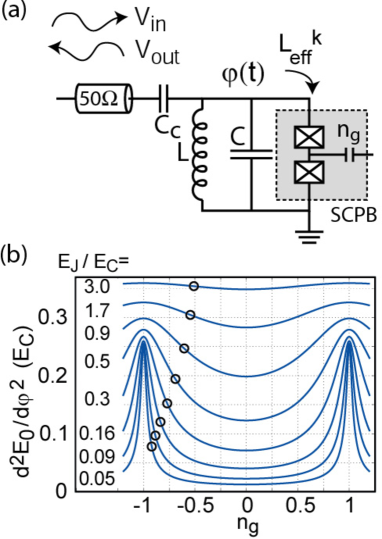
Figure 2: (a) Schematics of the capacitively coupled ”L-SET” inductive rf-electrometer. The resonance frequency $f_{p}^{-1}=2\pi\sqrt{(L\parallel L_{\mathrm{eff}}^{k})C}$ depends on the SCPB Josephson inductance $L_{\mathrm{eff}}^{k}$; (b) calculated modulation of the second $n_{g}$ - derivative (inverse $L_{\mathrm{eff}}^{0}$, see Eq. (3)) at the SCPB ground energy band, for different $E_{J}/E_{C}$, and $\varphi=0$. The circles mark optimal bias points for the electrometer operation.

The crucial number for electrometer operation is the differential modulation of $L_{\mathrm{eff}}$ (at the ground band), or dimensionless ”gain”:

$$g\equiv\frac{\partial}{\partial n_{g}}\left(\frac{L_{\mathrm{eff}}}{L_{\mathrm{eff,0}}}\right)\,,$$ (5)

which we have presented as normalized by $L_{\mathrm{eff,0}}$ which denotes the Josephson inductance at the special point $(n_{g}=\pm 1,\,\varphi=0)$. Using Eq. (2), we have $L_{\mathrm{eff,0}}=4L_{J0}$. For the best electrometer performance, $n_{g}$ should be biased at the points marked by circles in Fig. 2 (b). From Eq. (2) we also find the maximum gain $g_{m}$ which grows rapidly when $E_{J}/E_{C}\ll 1$: $g_{m}\simeq 2(E_{J}/E_{C})^{-1}$. Another important figure is the value of $L_{\mathrm{eff}}$ at the optimal gate bias which yields $g_{m}$, denoted here as $L_{\mathrm{eff,m}}$ AnalytNote . To some extent, the rapidly growing $L_{\mathrm{eff,m}}$ towards lowering $E_{J}/E_{C}$ (see Fig. 3) cancels the benefit of growing $g_{m}$ from the point of view of charge sensitivity.

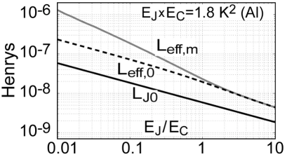
Figure 3: Numerical values of the SCPB ground band Josephson inductance $L_{\mathrm{eff,0}}$ (that at $n_{g}=\pm 1,\varphi=0$), and $L_{\mathrm{eff,m}}$ (at maximum gain, at $\varphi=0$) for a typical aluminium device. Also shown is the ”classical” Josephson inductance $L_{J0}$ in Eq. (1).

Without going into details, optimal charge sensitivity limited by zero-point fluctuations in the loaded $LC$-oscillator in Fig. 2 (a) is lsetsensit :

$$s_{q}^{\mathrm{QL}}=\frac{16\sqrt{2}e(L_{\mathrm{eff,m}})^{2}\sqrt{2k_{B}T_{N}}}{g_{m}\pi\sqrt{\hbar}\Phi_{0}L_{J0}\sqrt{Q_{i}}},$$ (6)

where $T_{N}$ is the noise temperature of the rf-amplifier, and $Q_{i}$ is the internal quality factor of the resonator. Evaluating the values in Eq. (6) numerically, we find that $s_{q}\sim 10^{-7}$e$/\sqrt{\mathrm{Hz}}$, order of magnitude better than the shot-noise limit of rf-SET, is intrinsically possible for the L-SET if $Q_{i}\sim 10^{3}$ and $T_{N}\sim 200$ mK. So far, the sensitivity in experiment lsetsensit ; MIKAthesis has been limited by $Q_{i}\lesssim 20$ down to $s_{q}\simeq 2\times 10^{-5}$e$/\sqrt{\mathrm{Hz}}$. The limit of Eq. (6) is reached when parameter values are chosen so that

$$\omega_{p}=\frac{\Phi_{0}^{2}(L_{\mathrm{eff,m}}+L)}{64\hbar L_{\mathrm{eff,m}}L}.$$ (7)

Equation (7) yields values typically $f_{p}=\omega_{p}/(2\pi)\simeq 1-2$ GHz, though dependence of $f_{p}$ is rather weak.

3 Quantum capacitance

The band energies of an SCPB depend on the (gate) charge $n_{g}$, see Fig. 1 (b), and the SCPB should then behave like a capacitance with respect to changes of $n_{g}$ Likharev85 ; AverinBruder03 , which means that the point of observation is at the gate electrode:

$$C_{\rm eff}^{k}=-\frac{\partial^{2}E_{k}(\varphi,n_{g})}{\partial V_{g}^{2}}=-\frac{C_{g}^{2}}{e^{2}}\frac{\partial^{2}E_{k}(\varphi,n_{g})}{\partial n_{g}^{2}}\,.$$ (8)

Phase modulation of the input capacitance $C_{\mathrm{eff}}(n_{g},\varphi)$ of the SCPB observed in this manner is plotted in Fig. 4 (b). As seen in the figure, $C_{\mathrm{eff}}$ has a strong phase dependence in the limit $E_{J}/E_{C}\gg 1$ around $\varphi=\pm\pi$. Exactly at $\varphi=\pm\pi$, Cooper-pair tunneling is completely blocked, and $C_{\mathrm{eff}}$ reduces to classical series capacitance of the junctions and $C_{g}$, that is, $\left[(C_{1}+C_{2})^{-1}+C_{g}^{-1}\right]^{-1}$.

The input capacitance depends sensitively (quadratically) on the coupling capacitance $C_{g}$, and even when $C_{g}$ is made unusually large such that it practically limits the charging energy, $C_{\mathrm{eff}}$ typically remains very small, in the femto-Farad range, see right hand scale of Fig. 4 (b). However, it has been suggested that the extremely strong phase dependence could be used for fast, reactively read phase detection Leif05 . This ”CSET” mode of operation is somewhat dual to the ”L-SET” electrometry.

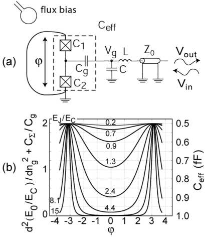
Figure 4: (a) Schematics of the experiment used to study how the SCPB appears as a tunable capacitance $C_{\mathrm{eff}}$; (b) left scale is the calculated second $n_{g}$-derivative of the SCPB ground band at $n_{g}=0$, and right scale is the corresponding effective capacitance if $C_{g}=1$ fF and $C_{\Sigma}=2$ fF.

An important figure of merit for phase sensitivity is the differential gain, analogous to Eq. (5):

$$f\equiv\frac{\partial}{\partial\varphi}\left(\frac{C_{\mathrm{eff}}}{C_{g}^{2}/(2C_{\Sigma})}\right)\,.$$ (9)

The maximum of $f$ w.r.t. $\varphi$ at $n_{g}=0$ is plotted in Fig. 5.

We consider the experimental setup of Fig. 4 (a), where the quantum capacitance $C_{\mathrm{eff}}$ is in parallel with a (generally much larger) stray capacitance $C$, and forms a resonator with an inductance $L$. In this scheme, it is typical to operate in the limit of vanishing internal dissipation which corresponds to change of phase $\Theta$ of the reflected carrier changing by $2\pi$ around the resonant frequency $f_{p}$.

Similarly as in the inductive readout, there are here no internal noise sources except quantum fluctuations in the resonator. Typically, therefore, sensitivity is again limited by noise of the preamplifier: spectral density of the voltage noise referred to preamplifier input is $s_{\mathrm{Vout}}=\sqrt{2k_{B}T_{N}Z_{0}}$, which can be regarded as a phase noise of the microwave carrier, $s_{\Theta}=s_{\mathrm{Vout}}/V_{\mathrm{out}}$. When the carrier amplitude is optimally large, it can be shown that under the conditions mentioned, $V_{\mathrm{out}}=\frac{e}{2C_{g}}Z_{0}\sqrt{\frac{C}{L}\frac{1}{2\pi}}$. When referred as an equivalent flux noise at detector input using Eq. (9), the result becomes

$$\begin{split}s_{\varphi}=&\frac{s_{\Theta}}{\partial\Theta/\partial\varphi}=2\sqrt{\pi}e\left(\frac{C}{C_{g}}\right)\frac{\sqrt{k_{B}T_{N}Z_{0}}}{f_{m}E_{C}}\\ &\simeq\frac{4\sqrt{\pi}C\sqrt{k_{B}T_{N}Z_{0}}}{f_{m}e}\,,\end{split}$$ (10)

where the last form follows from the assumption that at high $E_{J}/E_{C}$, charging energy is limited by the large gate capacitance. This is the ultimate limit with advanced junction fabrication (very thin oxide). The predicted phase sensitivity is plotted in Fig. 5. Evidently, sensitivity improves with decreasing stray capacitance $C$, since this results in larger modulation of total capacitance $C+C_{\mathrm{eff}}$. We see that $s_{\varphi}<10^{-6}$rad$/\sqrt{\mathrm{Hz}}$, far beyond an equally fast rf-SQUID, is possible in principle at high $E_{J}/E_{C}\sim 10$ and a low stray capacitance $C\sim C_{g}$.

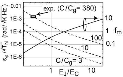
Figure 5: Left scale (dashed lines): Phase sensitivity predicted for the CSET, Eq. (10), first form, if $Z_{0}=50\,\Omega$ and $E_{C}=1$ K, for different ratios of the gate capacitance to stray capacitance. Right scale: the maximum gain $f_{m}$ of the phase detector. Experimental point is given by the rectangle (note that it had a larger capacitance ratio of $\sim 380$).

We investigated the discussed phase detection experimentally in the scheme of Fig. 4 (a), with the parameter values $E_{J}=0.30$ K, $E_{C}=0.83$ K, $E_{J}/E_{C}=0.36$, $C_{g}=0.65$ fF, $C=250$ fF, $C/C_{g}=380$, and $L=160$ nH. Except $C_{g}$, the sample parameters were determined by microwave spectroscopy cap . To the input bias coil of the phase detector, we applied low-frequency modulation by $0.013\,\Phi_{0}$ at 80 Hz. Its amplitude was calibrated relying on $\Phi_{0}$-periodicity of the static response. This way, we obtained a sensitivity of 1.3 mrad/$\sqrt{\textrm{Hz}}$, see the black curve in Fig. 6, limited by the 4 K amplifier noise, which figure is even better than expected (see Fig. 5).

We shall now discuss Fig. 6 in more detail. Both the curves were measured at a flux bias close to $\varphi\sim\pi$ which yields the largest gain $f_{m}$. For the black curve, $f(n_{g},\varphi)$ was further maximized by tuning $n_{g}$ close to 1, which also yielded a high level of low-frequency noise as can be seen in the data. Since the low-frequency noise is significantly reduced when we tuned $n_{g}=0$ where the response is insensitive to charge fluctuations (the gray curve), we assign the increased noise around $n_{g}=1$ to the ubiquitous low-frequency background charge noise.

Since the low-frequency noise at $n_{g}=0$ is free from the effect of charge noise, we were able to directly measure in the scheme the apparent flux noise, which we attribute to critical-current fluctuations. The power spectrum of the gray curve shows $1/f^{2}$ dependence in contrast to typical $1/f$ rule Clarke04 for big junctions. We convert this noise into fluctuations in critical current of either of the junctions, in other words, we ask the question: what would be the $I_{C}$ fluctuation $\Delta I_{C}=2e/\hbar(\Delta E_{J})$ in either one of the junctions which would cause a capacitance fluctuation $\Delta C_{\mathrm{eff}}$, and hence an apparent phase fluctuation $\Delta\varphi$ ? Equation (9) implies

$$\Delta C_{\mathrm{eff}}(n_{g},\varphi)=f(n_{g},\varphi)C_{0}\Delta\varphi\,,$$ (11)

where we have marked $C_{0}=C_{g}^{2}/(2C_{\Sigma})$. This then converts into $E_{J}$ fluctuation according to

$$\Delta E_{J}=\Delta C_{\mathrm{eff}}\left(\frac{\partial C_{\mathrm{eff}}}{\partial E_{J}}\right)^{-1}$$ (12)

We compute the partial derivative in Eq. (12) numerically; the result is $\frac{\partial C_{\mathrm{eff}}}{\partial E_{J}}\simeq 0.072\,\left(\frac{C_{g}}{e}\right)^{2}\frac{E_{C}}{E_{J}}\simeq 0.30\left(\frac{C_{g}}{e}\right)^{2}$. We also set $f(n_{g},\varphi)\rightarrow f_{m}$ since we had tuned to the maximum gain.

Finally, since the spectral densities of fluctuations are related similarly as the fluctuations itself, we have the amplitude spectrum of $I_{C}$ noise:

$$s_{IC}=\frac{2e}{\hbar}s_{EJ}=\frac{2e}{\hbar}f_{m}s_{\varphi}C_{0}\left(\frac{\partial C_{\mathrm{eff}}}{\partial E_{J}}\right)^{-1}\,.$$ (13)

This yields the gray line in Fig. 6, with the numbers around 10 Hz being comparable to big junctions.

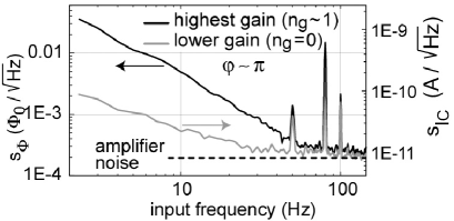
Figure 6: Measured equivalent flux noise at CSET input (left scale, black curve) and critical current noise (right scale, gray curve). Low-frequency flux modulalation by $0.013\,\Phi_{0,\mathrm{RMS}}$ at $80$ Hz was used as a marker.

References

• (1) A. Widom et. al., J. Low Temp. Phys. 57, 651 (1984).
• (2) D. V. Averin, A. B. Zorin, and K. Likharev, Sov. Phys. JETP 61, 407 (1985); K. Likharev and A. Zorin, J. Low. Temp. Phys. 59, 347 (1985).
• (3) D. V. Averin and C. Bruder, Phys. Rev. Lett. 91, 057003 (2003).
• (4) L. Roschier, M. Sillanpää, and P. Hakonen, Phys. Rev. B 71, 024530 (2005).
• (5) D. J. Flees, S. Han, and J. E. Lukens, Phys. Rev. Lett. 78, 4817 (1997).
• (6) M. Sillanpää, L. Roschier, and P. Hakonen, Phys. Rev. Lett. 93, 066805 (2004).
• (7) A. B. Zorin, Phys. Rev. Lett. 86, 3388 (2001).
• (8) R. J. Schoelkopf, P. Wahlgren, A. A. Kozhevnikov, P. Delsing, and D. E. Prober, Science 280, 1238 (1998).
• (9) Equation (2) does not allow for an analytical formula for $L_{\mathrm{eff,m}}$.
• (10) M. Sillanpää, L. Roschier, and P. Hakonen, Appl. Phys. Lett. 87, 092502 (2005).
• (11) M.A. Sillanpää, Ph.D. thesis, Helsinki University of Technology (2005); http://lib.tkk.fi/Diss/2005/isbn9512275686/.
• (12) M. A. Sillanpää, T. Lehtinen, A. Paila, Yu. Makhlin, L. Roschier, and P. J. Hakonen, Phys. Rev. Lett. 95, 206806 (2005).
• (13) F. C. Wellstood, C. Urbina, and J. Clarke, Appl. Phys. Lett. 85, 5296 (2004).