Synchronization Landscapes in Small-World-Connected Computer Networks Doctor of Philosophy Physics 5 György Korniss

Saroj K. Nayak Toh-Ming Lu Wayne G. Roberge Boleslaw K. Szymanski

July 2005
(For Graduation August 2005)

ACKNOWLEDGMENT

First and foremost I am deeply indebted to my academic and research adviser, Prof. György Korniss. I am particularly grateful for his guidance and support in the last four years of my life in Rensselaer. I thank Zoltán Toroczkai from Los Alamos National Laboratory for his mentorship when I was an intern in Center for Nonlinear Studies (Summer 2001) and Complex Systems group (Summer 2002). I also thank Mark Novotny and Zoltán Rácz for collaboration through fruitful discussions. Special thanks go to my thesis committee members, Prof. Szymanski, Prof. Lu, Prof. Roberge and Prof. Nayak.

I have benefited from time spent with group members and friends here at Rensselaer Polytechnic Institute. I would like to thank Balazs Kozma and Lauren O’Malley. I was particularly fortunate to have had Dr. Tansel Karabacak and Dr. Ibrahim Yilmaz as colleagues and close friends, with whom I have shared many interesting discussions, both academic and otherwise, since the day they accepted me as a guest in their house. Last, but not least, I also would like to thank dearest S. Azra Konet for her support for the last two months.

I acknowledge the financial support of the National Science Foundation (DMR-0113049) and Research Corporation (RI0761).

ABSTRACT

In this thesis we study synchronization phenomena in natural and artificial coupled multi-component systems, applicable to the scalability of parallel discrete-event simulation for systems with asynchronous dynamics. We also study the role of various complex communication topologies as synchronization networks. We analyze the properties of the virtual time horizon or synchronization landscape (corresponding to the progress of the processing elements) of these networks by using the framework of non-equilibrium surface growth.

When the communication topology mimics that of the short-range interacting underlying system, the virtual time horizon exhibits Kardar-Parisi-Zhang-like kinetic roughening. Although the virtual times, on average, progress at a nonzero rate, their statistical spread diverges with the number of processing elements, hindering efficient data collection. We show that when the synchronization topology is extended to include quenched random communication links (small-world links) between the processing elements, they make a close-to-uniform progress with a nonzero rate, without global synchronization. This leads to a fully scalable parallel simulation for underlying systems with asynchronous dynamics and short-range interactions. We study both short-range and small-world synchronization topologies in one- and two-dimensional systems. We also provide a coarse-grained description for the small-world-synchronized virtual-time horizon and compare the findings to those obtained by “simulating the simulations” based on the exact algorithmic rules. We also present numerical results for the evolution of the virtual-time horizon on scale-free Barabási-Albert networks serving as communication topology among the processing elements.

Finally, we investigate to what extent small-world couplings (extending the original local relaxational dynamics through the random links) lead to the suppression of extreme fluctuations in the synchronization landscape. In the absence of the random links, the steady-state landscape is “rough” (strongly de-synchronized state) and the average and the extreme height fluctuations diverge in the same power-law fashion with the system size (number of nodes). With small-world links present, the average size of the fluctuations becomes finite (synchronized state). For exponential-like noise the extreme heights diverge only logarithmically with the number of nodes, while for power-law noise they diverge in a power-law fashion. The statistics of the extreme heights are governed by the Fisher–Tippett–Gumbel and the Fréchet distribution for exponential and power-law noise, respectively.

Chapter 1 INTRODUCTION

1.1 Complex Networks

Cooperative behavior and collective phenomena have always been the center stage of statistical physics. More recently, the study of complex systems has become widespread across disciplines ranging from socio-economic systems, traffic models, epidemic models, to the Internet, the World-Wide Web, and grid computer networks. With the tools and frameworks provided by modern statistical physics, and with the availability of rapidly increasing computational resources, there is a chance to gain deeper understanding of the behavior of these systems.

One direction to study complexity is using minimal models where one considers a large number of simple interacting entities (agents, individuals, components, etc.) assuming a (typically simple) effective interaction between these entities. For example, in the Ising model for ferromagnets, the entities are the two-state spins and the interaction energetically prefers neighboring spins to be aligned. In simple models for social systems, the entities are humans, and the interaction can be, e.g., mimicking (simple majority influence by their social contacts).

While the interactions and the individual components may be simple, the collective behavior of these interacting systems are often far from trivial. For example, in the Ising model, in sufficiently high dimension, spontaneous order (symmetry breaking) emerges below some critical temperature. At the critical point the systems becomes strongly correlated, even though the interaction between spins only extends to a few neighbors. These are the kind of emergent behaviors we are interested in, namely, how locally interacting entities can produce large-scale effects. It needs to be emphasized that in these models, complexity emerges through the “outcome” of the evolution of the system with a large number of entities, not in the construction of the individual-level (“microscopic”) dynamics or rules.

Despite the great complexity and variety of systems, universal laws and phenomena are essential to our inquiry and to our understanding [1]. One way of describing complex systems is modeling them mathematically by using the framework of networks which is essentially a relational approach. A network can be defined as a set of items, referred to as nodes, and links connecting them. It is a concept borrowed from the graph theory, a subfield of combinatorics in mathematics.

The study of complex networks pervades various areas of science ranging from sociology to statistical physics [2, 3, 4]. Many of our important technological, information, and infrastructure systems can be considered complex networks [5, 6, 7, 8] with a large number of components. The links between the nodes in these networks facilitate some kind of effective interaction/dynamics between the nodes. Examples (with the processes inducing the interaction between the nodes) include high-performance scalable parallel or grid-computing networks (synchronization protocols for massive parallelization) [8], diffusive load-balancing schemes (relocating jobs among processors) [9], the Internet (protocols for sending/receiving packets) [5, 6, 10], the World Wide Web (hyperlinks in the web pages for other web pages) [11], the electric power grid (generating/transmitting power between generators and buses) [7], metabolic networks (reactions between molecules) [12] or social networks (acquaintance or social contacts) [13, 14]. Many of these systems are autonomous (by design or historical evolution), i.e., they lack a central regulator. Thus, fluctuations in the “load” in the respective network (data/state savings or task allocation in parallel simulations, traffic in the Internet, voltage/phase in the electric grid etc.) are determined by the collective result of the individual decisions of many interacting “agents” (nodes). As the number of processors on parallel architectures increases to hundreds of thousands [15], grid-computing networks proliferate over the Internet [16, 17], or the electric power-grid covers, e.g., the North-American continent [7], fundamental questions on the corresponding dynamical processes on the respective underlying networks must be addressed.

Regular lattices are commonly used to study physical systems with short-range interactions. Earlier studies focused mostly on the topological properties of the networks. Recent works, motivated by a large number of natural and artificial systems, such as the ones listed above, have turned the focus to processes on networks, where the interaction and dynamics between the nodes are facilitated by a complex network. The question then is how this possibly complex interaction topology influences the collective behavior of the system.

A common property of many real-life networks is that the degree or connectivity (number of connections of a node) follow a scale-free (power-law) distribution. Examples include world wide web, router level Internet, movie actors collaboration network, science collaboration network, cellular networks and linguistic networks [2]. Barabási and Albert [5] introduced a growth model with preferential attachment producing scale-free networks. They added one node at every time step with $m$ links and connected this node to existing nodes with a probability proportional to the degree of the existing nodes. This method leads to a power-law degree distribution function (having a heavier tail compared to an exponential one), $P(k)$$=$$\frac{2m^{2}}{k^{3}}$, shown in Fig. 1.1(a). The consequence of the power-law tail in the degree distribution is the existence of hubs, i.e., a few nodes with a large number of connections, often observed in real-life networks.

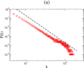
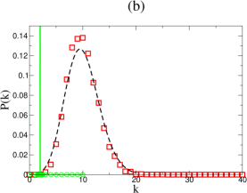
Figure 1.1: (a) Degree distribution of the scale-free Barabási-Albert network with $m$$=$$5$, yielding an average degree of $\langle k\rangle$$=$$10$. The dashed line shows the power-law behavior in log-log scale. (b) Degree distribution of a SW network (Erdős-Rényi Network on a 1D ring) with $p$$=$$8$. This $p$ value with the additional two nearest-neighbor links yields an average degree $\langle k\rangle$$=$$10$. The dashed curve is a Poissonian. The delta-function with circles around $\langle k\rangle$$=$$2$ is the degree distribution of the regular one-dimensional short-range network with only two nearest-neighbor links.

Watts and Strogatz, inspired by a sociological experiment [18], have proposed a network model known as the small-world (SW) network [19]. The SW concept describes the observation that, despite their often large size, there is a relatively short path between any two nodes in most networks with some degree of randomness. The SW model was originally constructed as a network to interpolate between regular lattices and completely random networks [20]. Watts and Strogatz considered a regular short-range network with $k$ nearest links per node. Then they randomly visited the links and rewired them to randomly chosen nodes with probability $p$. Thus, by varying the parameter $p$ they were able to interpolate between a regular ($p$$=$$0$) and a completely random ($p$$=$$1$) network.

Another way of constructing the SW network, instead of rewiring, is visiting every pair of nodes and adding a link between them with probability $p/N$, where $N$ is the number of nodes. This construction on top of the regular network, also called random graph and first introduced by Erdős and Rényi [20], have been traditionally used to describe the networks of random topology. The degree distribution of this SW graph is a Poissonian centered at the mean degree, $\langle k\rangle$$\simeq$$p+2$, as shown in Fig. 1.1(b) with $p$$=$$8$. For $p$$=$$0$, we obtain the short-range regular network with a Kronecker-delta degree distribution, $P(k)$$=$$\delta_{kz}$ where $z$ is the coordination number (in 1D, $z$$=$$2$, see Fig. 1.1(b)).

Another important characteristic of networks is the average shortest path length $\delta_{avg}$. The shortest path length can be defined as the minimum number of intermediary nodes between two nodes. All networks with some degree of randomness has the property that $\delta_{avg}$ is much smaller than that of regular network with the same number of nodes and with the same average degree. This very short separation between any pair of nodes is commonly referred to as the “low degree of separation”. Typically the average shortest path length increases no faster than the logarithm of the number of nodes $N$. For illustration we show the average shortest path length as a function of system size $N$ for SW ($p$$=$$8$) and BA ($m$$=$$5$) network in Fig. 1.2. Note that on a $d$-dimensional regular network $\delta_{avg}\sim N_{nodes}^{1/d}\sim N_{linear}$ where $N_{nodes}$ is the number of nodes, $N_{linear}$ is the linear system size ($N_{nodes}$$=$$N_{linear}^{d}$) and $d$ is the dimension.

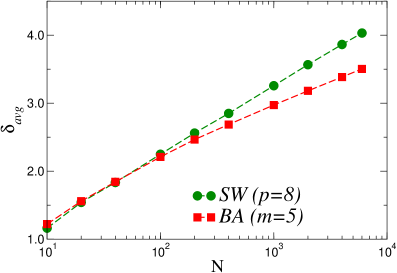
Figure 1.2: The average shortest path length $\delta_{avg}$ as a function of system size $N$ for SW ($p$$=$$8$) and BA ($m$$=$$5$). Note normal-log scale.

Systems and models (with well-known behaviors on regular lattices) have been studied on SW networks, such as the Ising model [21, 22, 23, 24], the XY model [25], phase ordering [26], the Edwards-Wilkinson model [27, 28, 29] and diffusion [27, 28, 29, 30, 31, 32, 33, 34]. Closely related to phase transitions and collective phenomena is synchronization in coupled multi-component systems [35]. SW networks have been shown to facilitate autonomous synchronization which is an important feature of these networks from both fundamental and system-design points of view [36, 37, 38]. In this thesis we study a synchronization problem which emerges [39] in certain parallel/distributed algorithms referred to as parallel discrete-event simulation (PDES) [40, 41, 42, 43]. First, we find that constructing a SW-like synchronization network for PDES can have a huge impact on the scalability of the algorithm [8]. Secondly, since the particular problem is effectively “local” relaxation in a noisy environment in a SW network, our study also contributes to the understanding of collective phenomena on these networks.

1.2 Parallel Discrete-Event Simulation

Simulation of large spatially extended complex systems in physics, engineering, computer science, or military applications require vast amount of CPU-time on serial machines using sequential algorithms. PDES enabled researchers to implement faithful simulations on parallel/distributed computer systems, namely, systems composed of multiple interconnected computers [40, 41, 42, 43]. Developing and implementing massively parallel algorithms is among the most challenging areas in computer/computational science and engineering [44]. While there are numerous technological and hardware-related points, e.g., concerning efficient message passing and fast communications between computer nodes, the theoretical algorithmic challenge is often as important.

PDES is a subclass of parallel and distributed simulations in which changes in the components of the system occur instantaneously from one state to another. In physics, chemistry and biology communities these types of simulations are most commonly referred to as dynamic or kinetic Monte Carlo simulations [45]. Examples of such simulation systems include cellular communication networks [42, 46], magnetic systems [47, 48], spatial epidemic models [49], thin-film growth [50, 51], battle-field models [52], and internet traffic models [53]. In these simulations the discrete events are call arrivals, spin-flip attempts, infections, monomer depositions, troop movements, and packet transmissions/receptions respectively. In these simulations the algorithm must faithfully and reproducibly keep track of the asynchrony of the local updates in the system’s configuration. For example standard random-sequential Monte Carlo simulations naturally produce Poisson asynchrony. In fact, such continuous-time simulations (e.g., single spin-flip Glauber dynamics [54]) were long believed to be inherently serial until Lubachevsky’s illuminating work [55, 56] on the parallelization of these simulations without altering the underlying dynamics. The essence of the problem is to algorithmically parallelize “physically” non-parallel dynamics of the underlying system while enforcing causality between events and reproducibility. This requires some kind of synchronization to ensure causality between events processed by different processing elements (PEs).

The two basic ingredients of PDES are the set of local simulated times (or virtual times [57]) and a synchronization scheme [40]. The difficulty in PDES is that the discrete events are not synchronized by a global clock, since the dynamic is usually asynchronous. There are two main approaches in PDES: (i) conservative synchronization, which avoids the possibility of any type of causality errors by checking if each event is safe to process [58, 59] and (ii) optimistic synchronization, which allows causality errors, then initiates rollbacks to correct the erroneous computations [57, 60]. Innovative methods have also been introduced to make optimistic synchronization more efficient, such as reverse computation [61]. Other recent improvements to exploit parallelism in discrete event systems are the “lookback” method [62] and the freeze-and-shift algorithm [63].

A PDES should have the following properties to be scalable [46]: First, a scalable PDES scheme must ensure that the average progress rate of the simulation approaches a nonzero constant in the long-time limit as the number of PEs, $N_{PE}$, goes to infinity (computational scalability) . Second, the “width” of the simulated time horizon (the spread of the progress of the individual PEs) should be bounded as $N_{PE}$ goes to infinity (measurement scalability) [64]. The second requirement is crucial for the measurement phase of the simulation to be scalable to avoid long delays while waiting for “slow” nodes [50] or, alternatively, to eliminate the need to reserve a large amount of memory for temporary data storage: a large width of the virtual time horizon hinders scalable data management. Temporarily storing a large amount of data on each PE (being accumulated for “on-the-fly” measurements) is limited by available memory while frequent global synchronizations can get costly for large $N_{PE}$. Thus, one aims to devise a scheme where the PEs make a nonzero and close-to-uniform progress without global synchronization. In such a scheme, the PEs autonomously learn the global state of the system (without receiving explicit global messages) and adjust their progress rate accordingly. In this thesis we study regular and SW network communication topologies and show a possible way to construct fully scalable parallel algorithms for underlying systems with asynchronous dynamics and short-range interactions on regular lattices.

Since one is interested in the dynamics of the underlying complex system, the PDES scheme must simulate the “physical time” variable of the complex system. When the simulations are performed on a single processor machine, a single (global) time stream is sufficient to “label” or time-stamp the updates of the local configurations, regardless whether the dynamics of the underlying system is synchronous or asynchronous. When simulating asynchronous dynamics on distributed architectures, however, each PE generates its own physical, or virtual time, which is the physical time variable of the particular computational domain handled by that PE. As a result of the local stochastic time increments and the synchronization dynamics, at a given wall-clock instant the simulated virtual times of the PEs can differ, a phenomenon called “time horizon roughening”. We denote the simulated, or virtual time at PE $i$ measured at wall-clock time $t$, by $\tau_{i}(t)$. The wall-clock time $t$ is directly proportional to the (discrete) number of parallel steps simultaneously performed on each PE, also called the number of Monte-Carlo steps (MCS) in dynamic Monte Carlo simulations. Without altering the meaning, $t$ from now on will be used to denote the number of discrete steps performed in the parallel simulation. The set of virtual times $\{\tau_{i}(t)\}_{i=1}^{N_{PE}}$ forms the virtual time horizon (synchronization landscape) of the PDES scheme after $t$ parallel updates.

The design of efficient parallel-update schemes is a rather challenging problem, due to the fact that the dynamics of the simulation scheme itself is a complex system where the specific synchronization rules correspond to the “microscopic dynamics”, and its properties are hard to deduce using classical methods of algorithm analysis. Here we present a less conventional approach to the analysis of efficiency and scalability for the class of massively parallel conservative PDES schemes, by mapping the parallel computational process itself onto a non-equilibrium surface growth model [39]. Then, using methods from statistical mechanics to study the dynamics of such surfaces (in a completely different context), we solve the scalability problem of the computational PDES scheme [8, 39]. Similar connections between phase transitions and computational complexity have recently been made [65, 66] for rollback-based (or optimistic) PDES algorithms [57] and self-organized criticality [67, 68]. These connections have turned out to be highly fruitful to gain more insight into traditionally hard computational problems [69, 70]. In this thesis we consider the scalability of conservative synchronization schemes for self-initiating processes [71, 72], where update attempts on each node are modeled as independent Poisson streams and are independent of the configuration of the underlying system [55, 56]. We study the morphological properties of the virtual time horizon. Although these properties simplify the analysis of the corresponding PDES schemes, they can be highly efficient [47] and are readily applicable to a large number problems in science and engineering. Further, the performance and the scalability of these PDES schemes become independent of the specific underlying system i.e., we learn the generic behavior of these complex computational schemes. Through our study one also gains some insight into the effects of SW-like interaction topologies on the critical fluctuations in interacting systems.

This thesis is organized as follows. In Chapter 2 we show detailed results for the short-range model on one and two-dimensional regular networks with nearest-neighbor communication, which we refer to as the basic conservative synchronization (BCS) scheme [39]. In Chapter 3 we extend our study to SW networks, constructed by adding random links to regular networks [8]. Chapter 4 presents the results on scaling and distributions of the extreme fluctuations in regular and SW networks. In Chapter 5 we summarize our work and discuss future directions.

Chapter 2 SYNCHRONIZATION IN REGULAR NETWORKS

First, we briefly summarize the basic observables relevant to our analysis of synchronization and the scaling relations borrowed from non-equilibrium surface growth theory. The set of local simulated times for the PEs, $\{\tau_{i}(t)\}_{i=1}^{N_{PE}}$, constitutes the simulated time horizon. Here $N_{PE}$ is the number of PEs and $t$ is the discrete number of parallel steps, directly related to real (wall-clock) time. On a regular $d$-dimensional hypercubic lattice $N_{PE}$=$N^{d}$, where $N$ is the linear size of the lattice and $d$ is the dimension. For a one-dimensional system $N_{PE}$=$N$. In the rest of the thesis we will use the term “height”, “simulated time”, or “virtual time” interchangeably, since we refer to the same local observable (local field variable).

Since the discrete events in PDES are not synchronized by a global clock, the processing elements have to communicate with others for synchronization. One of the first approaches to this problem for self-initiating processes is the basic conservative synchronization (BCS) scheme proposed by Lubachevsky [55, 56] by using only nearest neighbor interactions mimicking [39] the interaction topology of the underlying physical system. His basic model associated each component or site with one PE (worst-case scenario) under periodic boundary conditions. In this BCS scheme, at each time step only those PEs whose local simulated time is not larger than the local simulated times of their next nearest neighbors are incremented by an exponentially distributed random amount so that the discrete events exhibit Poisson asynchrony. Namely, a PE will only perform its next update if it can obtain the correct information to evolve the local configuration (local state) of the underlying physical system it simulates, without violating causality. Hence, the evolution equation for site $i$ simply becomes

$$\tau_{i}(t+1)=\tau_{i}(t)+\eta_{i}(t)\Theta(-\phi_{i}(t))\Theta(\phi_{i+1}(t))\;,$$ (2.1)

where $\eta_{i}(t)$ is an exponentially distributed random number, $\Theta(...)$ is the Heaviside step-function and $\phi_{i}(t)=\tau_{i}(t)-\tau_{i-1}(t)$ is the local slope. In one-dimension with periodic boundary conditions, the network has a ring topology as shown in Fig. 2.1(a),

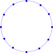
Figure 2.1: One-dimensional (1D) regular network (with periodic boundary conditions), where nodes are connected to their nearest neighbors.

so each node is connected to the nearest left and right neighbors. The nearest-neighbor interaction in the BCS scheme implies that in order to ensure causality, PEs need to exchange information on their local simulated (virtual) times only with neighboring PEs in the virtual network topology. The possible configurations for the local simulated times for the successive nodes are shown in Fig. 2.2.

Figure 2.2: Possible simulated-time configurations for three successive nodes (involving two successive slopes) in the basic conservative scheme (BCS) in one dimension. From the perspective of node $i$, only configuration (b) allows it to proceed (node $i$ is a local minimum). In all other cases causality could be violated if an update occurs at site $i$, because the local field variables of the neighboring nodes are not known at the instant of update attempt.

In these configurations update occurs only if the node we are considering (node $i$) is a local minimum. In the other three cases the node $i$ idles. In analyzing the performance of the above scheme, it is helpful that the progress of the simulation itself is decoupled from the possibly complex behavior of the underlying system. This is contrary to optimistic approaches, where the evolution of the underlying system and the progress of the PDES simulation are strongly entangled [65], making scalability analysis a much more difficult task.

One of the important aspects of conservative PDES is the theoretical efficiency or utilization which can be defined simply as the average fraction of non-idling PEs. It also determines the average progress rate of the simulation. In the BCS where only nearest-neighbor interactions are present, the utilization is equal to the density of local minima in the simulated time horizon. On a regular one-dimensional lattice, it can be defined as

$$\left\langle u(N,t)\right\rangle=\frac{1}{N}\sum_{i=1}^{N}\left\langle\Theta(\tau_{i-1}-\tau_{i})\Theta(\tau_{i+1}-\tau_{i})\right\rangle=\frac{1}{N}\sum_{i=1}^{N}\left\langle\Theta(-\phi_{i})\Theta(\phi_{i+1})\right\rangle\;,$$ (2.2)

where $\phi_{i}$$=$$\tau_{i}-\tau_{i-1}$ is the local slope, $\Theta(...)$ is the Heaviside step function, and $\left\langle...\right\rangle$ denotes an ensemble average. Note that the individual terms in the sum in Eq. (2.2), $\left\langle\Theta(-\phi_{i})\Theta(\phi_{i+1})\right\rangle$, become independent of $i$ for a system of identical PEs due to translational invariance.

Another important observable of PDES is the statistical spread or width of the simulated time surface. The measurement scalability of the PDES scheme, is characterized by the width. Instead of dealing with the actual spread (difference between the maximum and minimum values) we shall consider the average “width”, $w$. It is defined as the root-mean-square fluctuation of the virtual times measured from the mean, $w=\sqrt{\langle w^{2}\rangle}$, where

$$\left\langle w^{2}\right\rangle\equiv\left\langle w^{2}(N,t)\right\rangle=\left\langle\frac{1}{N^{d}}\sum_{i=1}^{N^{d}}\left[\tau_{i}(t)-\bar{\tau}(t)\right]^{2}\right\rangle\;\;,$$ (2.3)

with $\bar{\tau}(t)$$=$$(1/N^{d})\sum_{i=1}^{N^{d}}\tau_{i}(t)$ being the mean progress (“mean height”) of the time surface, and $d$ is the dimension.

As we mentioned in Chapter 1, for the PDES scheme to be fully scalable, the following two criteria must be met: (i) the virtual time horizon must progress on average at a nonzero rate, and (ii) the typical spread of the time horizon should be finite, as the number of PEs $N$ goes to infinity. When the first criterion is ensured for large enough times $t$, the simulation is said to be computationally scalable, meaning that when increasing the size of the network to infinity, while keeping the average computational domain/load on a single PE the same, the simulation will progress at a nonzero rate. However, as we will show below, while increasing the system size, the spread in the time horizon can diverge, severely hindering frequent data collection about the state of the simulated system. Specifically, when one requires to take a measurement of some physical property of the simulated system at virtual time $\tau$, PEs have to wait (in wall-clock time) until all the virtual simulated times at all the PEs pass through the value of $\tau$. Thus, in order to collect system-wide measurements from the simulation, we incur a waiting time proportional to the spread, or width of the fluctuating time horizon. For PDES schemes for which the spread diverges with system size, the waiting time for the measurements will also diverge, and the scheme is not measurement scalable. When condition (ii) is fulfilled for large enough times $t$, we say that the PDES scheme is measurement scalable.

2.1 Scaling in non-equilibrium surfaces

Since we use the formalism and terminology of non-equilibrium surface growth phenomena, we briefly review scaling concepts for self-affine or rough surfaces. The scaling behavior of the width, $\langle w^{2}(N,t)\rangle$ where $N$ is the linear system size and $t$ is the time, alone typically captures and identifies the universality class of the non-equilibrium growth process [73, 74, 75]. In a finite system, the width initially grows as $\left\langle w^{2}(N,t)\right\rangle\sim t^{2\beta}$. After a system-size dependent cross-over time $t_{\times}\sim{N}^{z}$, it reaches a steady-state $\left\langle w^{2}(N,t)\right\rangle\sim{N}^{2\alpha}$ for $t\gg t_{x}$. In expressions above $\alpha$, $\beta$ and $z$=$\alpha/\beta$ are called the roughness, the growth, and the dynamic exponents, respectively. The above behavior can be summarized as follows

$$\left\langle w^{2}(N,t)\right\rangle\sim\left\{\begin{array}[]{ll}t^{2\beta}&\mbox{for $t$$\ll$$t_{x}$}\\ N^{2\alpha}&\mbox{for $t$$\gg$$t_{x}$}\end{array}\right.\;,$$ (2.4)

where $t_{x}$$\sim$$N^{z}$ is the cross-over time. From this scaling, one can also extract a length-scale, known as lateral correlation length, $\xi\sim t^{1/z}$ for times less than $t_{x}$, reaching the system size at the cross-over time. The temporal and system-size scaling of the width exhibited by Eq. (2.4) can be captured by the Family-Vicsek [76] relation,

$$\left\langle w^{2}(N,t)\right\rangle=N^{2\alpha}f(t/N^{z})\;.$$ (2.5)

Note that the scaling function $f(x)$ depends on $t$ and the linear system-size $N$ only through the specific combination, $t/N^{z}$, reflecting the importance of the crossover time $t_{\times}$. For small values of its argument $f(x)$ behaves as a power law, while for large arguments it approaches a constant

$$f(x)\sim\left\{\begin{array}[]{ll}x^{2\beta}&\mbox{if $x$$\ll$$1$}\\ \mbox{const.}&\mbox{if $x$$\gg$$1$}\end{array}\right.\;,$$ (2.6)

yielding the correct scaling behavior of the width for early times and for the steady-state, respectively.

A somewhat less frequently studied quantity is the growth rate of a growing surface. This quantity is typically non-universal [39, 77, 78, 79, 80, 81, 82], but as was shown by Krug and Meakin [78], on $d$-dimensional regular lattices, the finite-size corrections to it are. In the context of the basic PDES scheme, the growth rate of the simulated time surface corresponds to the progress rate (or utilization) of the simulation, hence our special interest in this observable. For the finite-size behavior of the steady-state growth rate, one has [78]

$$\langle u(N)\rangle\simeq\langle u(\infty)\rangle+\frac{const.}{N^{2(1-\alpha)}}\;,$$ (2.7)

where $\langle u(\infty)\rangle$ is the value of the growth rate in the asymptotic infinite system-size limit and $\alpha$ is the dimension-dependent roughness exponent of the growth process.

2.2 One-Dimensional Basic Conservative Synchronization Network

Based on a mapping between virtual times and surface site heights [39] and on the analogy with the single-step surface growth model [83], in the coarse-grained description [77], the virtual time horizon of the BCS is proposed to be governed by the Kardar-Parisi-Zhang (KPZ) equation [84], well-known in surface growth phenomena

$$\partial_{t}\hat{\tau}_{i}=\nabla^{2}\hat{\tau}_{i}-\lambda(\nabla\hat{\tau}_{i})^{2}+...+\eta_{i}(t)\;,$$ (2.8)

where $\nabla^{2}\hat{\tau}_{i}$ is the discretized Laplacian, $\nabla^{2}\hat{\tau}_{i}=\hat{\tau}_{i+1}+\hat{\tau}_{i-1}-2\hat{\tau}_{i}$, $\nabla\hat{\tau}_{i}$ is the discretized gradient, $\nabla\hat{\tau}_{i}=\hat{\tau}_{i+1}-\hat{\tau}_{i}$, $\hat{\tau}_{i}(t)=\tau_{i}-\bar{\tau}$ is the surface height fluctuation (or virtual time) measured from the mean, $\eta_{i}(t)$ is Gaussian noise delta-correlated in space and time, $\langle\eta_{i}(t)\eta_{j}(t^{\prime})\rangle=2D\delta_{ij}\delta(t-t^{\prime})$, $\lambda$ is a positive constant, and $...$ stands for higher order irrelevant terms. Equation (2.8) can also give an account of a number of other nonlinear phenomena such as Burgers turbulence [85] and directed polymers in random media [73]. When the simple update rule of the basic synchronization scheme is implemented on a one-dimensional network, one can observe a simulated time surface governed by the KPZ equation, and in the steady-state, by an Edwards-Wilkinson Hamiltonian [86] [Fig. 2.3(a)].

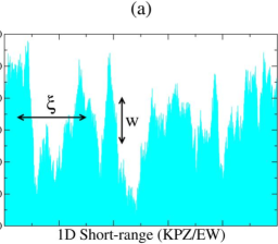
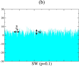
Figure 2.3: Virtual time horizon snapshots for 10,000 sites in 1D. (a) For the regular network with nearest-neighbor connections ($p$=$0$). The lateral correlation length $\xi$ and width $w\equiv\sqrt{w^{2}}$ are shown for illustration in the graph. The rough steady-state surface belongs to the KPZ/EW universality class. (b) For the SW synchronization network. The heights are effectively decorrelated and both the correlation length and the width are reduced, and approach system-size independent values for sufficiently large systems. The resulting surface is macroscopically smooth. Note that the heights are relative to the average height.

When analyzing the statistical and morphological properties of the stochastic landscape of the simulated times, it is convenient to study the height-height correlation or its Fourier transform, the height-height structure factor. The equal-time height-height structure factor $S(k,t)$ in one-dimension is defined through

$$N\delta_{k,-k^{\prime}}S(k,t)=\langle\tilde{\tau}_{k}(t)\tilde{\tau}_{k^{\prime}}(t)\rangle\;,$$ (2.9)

where $\tilde{\tau}_{k}=\sum_{j=1}^{N}e^{-ikj}\hat{\tau}_{j}$ is the Fourier transform of the virtual times with the wave number $k$=$2\pi n/N$, $n$=$1,2,...,N-1$ and $\delta_{k,-k^{\prime}}$ is the Kronecker delta. The structure factor essentially contains all the “physics” needed to describe the scaling behavior of the time surface. Here we focus on the steady-state properties ($t$$\to$$\infty$) of the time horizon where the structure factor becomes independent of time, $\lim_{t\to\infty}S(k,t)$$=$$S(k)$. In the long-time limit, in one dimension, for a KPZ surface described by Eq. (2.8) one has (see Appendix A) [77]

$$S(k)=\frac{D}{2[1-\cos(k)]}\sim\frac{1}{k^{2}}\;,$$ (2.10)

where $D$ is a constant and the latter approximation holds for small values of $k$. By performing the inverse Fourier transformation of Eq. (2.10), we can also obtain the spatial two-point correlation function,

$$G(l)=\frac{1}{N}\sum_{i=1}^{N}G_{i,i+l}=\frac{1}{N}\sum_{k\neq 0}e^{ikl}S(k)\;,$$ (2.11)

where $G_{i,i+l}$$=$$\langle(\tau_{i}-\bar{\tau})(\tau_{i+l}-\bar{\tau})\rangle$ is the site-dependent two point function, yielding [77, 87]

$$G(l)\simeq\frac{D}{2}\left(\frac{N}{6}-l\right)$$ (2.12)

for $1\ll l\ll L$. In particular, for the steady-state width one finds

$$\langle w^{2}\rangle=\frac{1}{N}\sum_{k\not=0}S(k)=G(0)\simeq\frac{D}{12}N\sim N$$ (2.13)

in one dimension [77]. This divergent width is caused by a divergent length scale, $\xi$, the “lateral” correlation length in the KPZ-like synchronization landscape.

The measured steady-state structure factor [Fig. 2.4(a)], obtained by simulating the BCS based on the exact rules for the evolution of the synchronization landscape confirms the coarse-grained prediction for small $k$ values, $S(k)\sim 1/k^{2}$. Figure 2.4(b) shows the corresponding spatial two-point correlation function, $G(l)$.

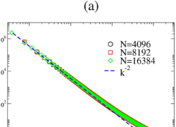
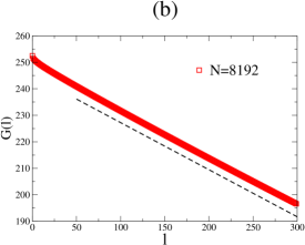
Figure 2.4: (a) The steady-state structure factor as a function of the wave number for the BCS scheme in 1D. The small-$k$ course-grained prediction (consistent with the steady-state EW/KPZ universality class in 1D) is indicated by a dashed line [Eq. (2.10)]. Note the log-log scales. (b) Steady-state spatial two-point correlation function. The straight line again indicates the asymptotic EW/KPZ behavior in one dimension [Eq. (2.12)].

Simulation of the BCS scheme in one dimension yields scaling exponents that agree within error of the predictions of the KPZ equation [73, 74, 84]. The time evolution of the width [Fig. 2.5(a)] shows that the growth exponent $\beta\simeq 1/3$.

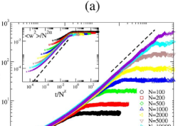
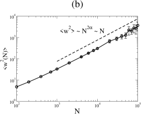
Figure 2.5: (a) Time evolution of the width for different system-sizes in the BCS scheme in 1D. The dynamics of the evolution of the virtual times is governed by the KPZ equation. The inset shows the same data on scaled axes, $\langle w^{2}\rangle/N^{2\alpha}$ versus $t/N^{z}$. Each curve has been obtained by averaging over at least fifty realizations. (b) The steady-state width of the time horizon for the one-dimensional BCS as a function of system-size. The dashed straight line represents the asymptotic one-dimensional KPZ/EW behavior, $\left\langle w^{2}(N)\right\rangle\sim N^{2\alpha}$ with $\alpha$=$1/2$.

Looking at the system-size dependence of the steady-state width [Figure 2.5(b)], we find the roughness exponent $\alpha\simeq 1/2$, consistent with the one-dimensional KPZ value, $\langle w^{2}\rangle\sim N^{2\alpha}\sim N$. The dynamic exponent values found from the width as a function of the cross-over time and $z$=$\alpha/\beta$ are the same, about $3/2$. The inset in Fig. 2.5(a) shows that the scaled version of the width evolution by using the scaling exponents is consistent with the Family-Vicsek relation [Eq. (2.5)], although with relatively large corrections to scaling.

The steady-state width distributions, $P(w^{2})$, have been introduced to provide a more detailed characterization of surface growth processes [88, 89, 90, 91] and have been used to identify universality classes [39]. Note that the width

$$w^{2}=\frac{1}{N^{d}}\sum_{i=1}^{N^{d}}[\tau_{i}(t)-\bar{\tau}(t)]^{2}\;,$$ (2.14)

itself is a fluctuating quantity. The width distribution for the EW (or a steady-state one-dimensional KPZ) class is characterized by a universal scaling function, $\Phi(x)$, such that $P(w^{2})=\langle w^{2}\rangle^{-1}\Phi(w^{2}/\langle w^{2}\rangle)$, where $\Phi(x)$ can be calculated analytically for a number of models, including the EW class [88]. The width distribution for the basic synchronization scheme is shown in

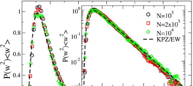
Figure 2.6: ]

Scaled width distributions for the BCS scheme in 1D. The exact asymptotic EW/KPZ width distribution [88] is shown with a dashed line. The inset shows the same distributions on log-normal scales.

Fig. 2.6. Systems with $N\geq 10^{3}$ show convincing data collapse onto this exact scaling function. The inset in Fig. 2.6 shows the same graph in log-normal scale to show the collapse at the tail of the distribution. The convergence to the limit distribution is very slow when compared to other microscopic models (such as the single-step model [73, 91]) belonging to the same KPZ universality class.

Now we discuss our findings for the steady-state utilization of the BCS scheme. As stated above, the synchronization landscape of the virtual times belongs to the EW universality class in one dimension. This implies that the local slopes in the steady-state landscape are short-range correlated [77]. Hence the density of local minima in the synchronization landscape, and in turn the utilization, remains nonzero in the infinite system-size limit [39, 77]. For a fixed $N$, the utilization drops from relatively higher initial value at early times to its steady-state value in a very short time [Fig. 2.7(a)]. Further, the steady-state utilizations for various systems converge to the asymptotic system-size independent value.

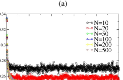
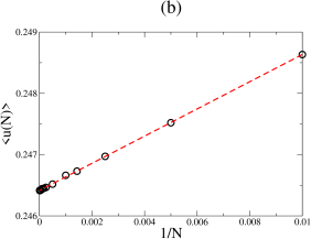
Figure 2.7: (a) Utilization in the 1D BCS scheme as a function of time for various system sizes. (b) Steady-state utilization as a function of the $1/N^{2(1-\alpha)}$ as suggested by Eq. (2.7) with the 1D KPZ roughness exponent $\alpha$$=$$1/2$. The dashed line is a linear fit, $\langle u(N)\rangle\approx 0.2464+0.2219/N$

In 1D, since $\alpha$$=$$0.5$ the utilization, by using Eq. (2.7) as a function of system size, becomes

$$\langle u(N)\rangle\simeq\langle u(\infty)\rangle+\frac{const.}{N}$$ (2.15)

as shown in Fig. 2.7(b). For the KPZ model [Eq. (2.8)] $\langle u(\infty)\rangle=1/4$, since in the steady state the slopes are delta-correlated, resulting in a probability $1/4$ for the configuration in Fig. 2.2(b), corresponding to a local minimum. For the actual BCS synchronization profile $\langle u(\infty)\rangle\simeq 0.2464$ [39, 77], as a result of non-universal short-range correlations present for the slopes in the specific microscopic model [87] as can be seen in Fig. 2.8.

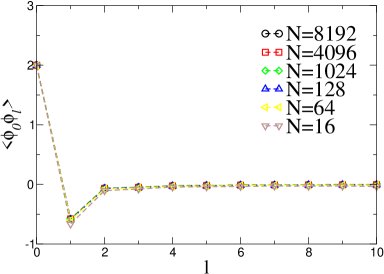
Figure 2.8: Slope-slope correlation function for the BCS scheme on a 1D short-range network for various system sizes.

In summary, we have shown that the 1D BCS time horizon belongs to the KPZ universality class as $N$ goes to infinity, then the measurement part of the 1D BCS scheme is not scalable.

2.3 Two-Dimensional Basic Conservative Synchronization Network

A natural generalization to pursue is the synchronization dynamics and the associated landscapes on the networks in higher dimensions. One might ask whether PDES of two-dimensional phenomena exhibit kinetic roughening of the virtual time horizon. Preliminary results indicated that this is the case [16, 92]. In this section we give detailed results when the BCS scheme is extended into a two-dimensional lattice in which each node has four nearest neighbors. We consider a system with periodic boundary conditions in both axes as can be seen in Fig. 2.9(a).

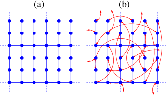
Figure 2.9: Communication topologies in 2D. (a) 2D regular network, where each node is connected to its four nearest neighbors. (b) SW synchronization network. One random link per node is added on top of the 2D regular network. Arrowed lines show the bidirectional random links between the nodes.

The same microscopic rules, i.e., each node increments its local simulated time by an exponentially distributed random amount when it is a local minima among its nearest neighbors, are applied to this lattice. As in the one-dimensional case, during the evolution of the local simulated times correlations between the nodes develop in the system. One observes a rough time surface in the steady-state of the 2D BCS network. Figure 2.10(a) shows the

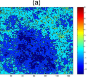
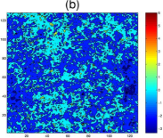
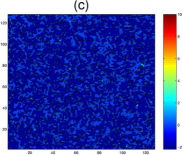
Figure 2.10: Synchronization landscapes as contour plots for the 2D BCS on regular and SW networks of 128x128 nodes. (a) for the BCS scheme on a regular lattice with only nearest-neighbor connections (equivalent to $p$=$0$); (b) for $p$=$0.1$; (c) for $p$=$1.0$.

contour plot of the simulated time surface for BCS scheme in 2D. In 2D as well, we observe kinetic roughening of the BCS scheme. The simulated time surface for a finite system roughens with time in a power-law fashion. It then saturates after some system-size dependent crossover time to its system-size dependent steady-state value, as shown in [Fig. 2.11(a)]. Our estimate for the growth exponent in the early-time regime is $\beta$$=$$0.125$, significantly smaller than that of one dimension.

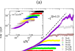
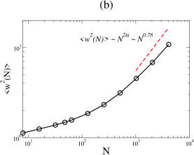
Figure 2.11: (a) Time evolution of the width in 2D BCS scheme. The dashed line indicates the power-law behavior of the width before saturation with a growth exponent $\beta$$\approx$$0.125$. The inset shows the scaled plot $\left\langle w^{2}\right\rangle/N^{2\alpha}$ vs. $t/N^{z}$. (b) Steady-state width of the 2D BCS scheme as a function of the linear system-size. The dashed line corresponds to the asymptotic 2D KPZ scaling with roughness exponent $2\alpha$$=$$0.78$ as obtained by high-precision simulations of the RSOS model [93]. Note the log-log scales.

The roughness exponent $\alpha$ for KPZ-like systems have been measured and estimated in a number of experiments and simulations [73]. Since exact exponents for the higher-dimensional KPZ universality class are not available, for reference, we compare our results to a recent high-precision simulation study by Marinari et al. [93] on the restricted solid-on-solid (RSOS) model [94], a model believed to belong to the KPZ class. They found in [93] that $\alpha$$\simeq$$0.39$ for the 2D RSOS roughness exponent. While our simulations of the virtual time horizon show kinetic roughening in Fig. 2.11(a), the scaled plot, suggested by Eq. (2.5), indicates very strong corrections to scaling for the BCS in 2D (inset). Figure  2.11(b) and Fig.2.12 also indicates that the (KPZ) scaling regime is approached very slowly in the steady-state, which is not completely unexpected: for the 1D BCS scheme as well, convergence to the steady-state roughness exponent [Fig. 2.5(a)] and to the KPZ width distribution [Fig. 2.5(b)] only appears for linear system sizes $N>{\cal O}(10^{3})$. Here, for the 2D case, the asymptotic roughness scaling [Fig. 2.11(b)] and width distribution [Fig. 2.12] has not been

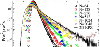
Figure 2.12: The scaled width distributions for the 2D BCS scheme. The solid curve is the asymptotic 2D KPZ scaled width distribution, again from high-precision RSOS simulations [95]. Note the log-normal scales.

reached for the system sizes we could simulate (up to linear system size $N$$=$$4096$). Nevertheless the trend in the finite-size behavior, and the identical microscopic rules (simply extended to 2D) suggest that 2D BCS landscape belongs to the 2D KPZ universality class.

For further evidence, we also constructed the structure factor for the 2D BCS steady-state landscape. As shown in Fig. 2.13(a), $S(k_{x},k_{y})$ exhibits a strong singularity about ${\bf k}$$=$${\bf 0}$.

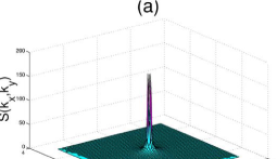
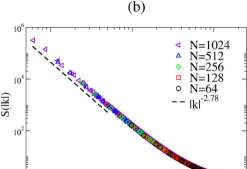
Figure 2.13: Structure factor for the BCS scheme in 2D. (a) as a function of the wave number components $k_{x}$ and $k_{y}$. (b) as a function of the magnitude of the wave number for different system-sizes. The dashed line shows the asymptotic 2D KPZ behavior for small values of $|\textbf{k}|$ [Eq. (2.16)] with $\alpha$$=$$0.39$ [93]. Note the log-log scales.

For further analysis, we exploited the symmetry of $S(k_{x},k_{y})$ that it can only depend on $|{\bf k}|=\sqrt{k_{x}^{2}+k_{y}^{2}}$. Hence, we averaged over all directions having the same wave number $|{\bf k}|$ to obtain $S(|{\bf k}|)$. For small wave numbers we found that it diverges as

$$S(|{\bf k}|)\sim\frac{1}{|{\bf k}|^{2+2\alpha}}\;,$$ (2.16)

with $\alpha=0.39$, as shown in Fig. 2.13(b). This is consistent with the small-$k$ behavior of the structure factor of the 2D KPZ universality class with roughness exponent $\alpha$$\simeq$$0.39$ [93]. As noted above, the scaling of the width and its distribution exhibited very slow convergence to those of our reference-KPZ system, the RSOS model [93, 95]. This is likely the effect of the non-universal and surprisingly large contributions coming from the large-$k$ modes, leading to very strong corrections to scaling for the system sizes we were able to study in 2D. Looking directly at the small-$|{\bf k}|$ behavior of $S(|{\bf k}|)$ is undisturbed by the larger-$|{\bf k}|$ modes, hence the agreement with the 2D KPZ scaling is relatively good.

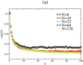
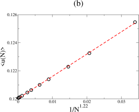
Figure 2.14: (a) The time evolution of the steady-state utilization in 2D BCS scheme for various system sizes. (b) The steady-state utilization in the 2D BCS scheme as a function of $1/N^{2(1-\alpha)}$ as suggested by Eq. (2.7) with the 2D KPZ roughness exponent $\alpha$$=$$0.39$. The dashed line is a linear fit, $\langle u(N)\rangle\approx 0.1201+0.1585/N^{1.22}$.

The steady-state utilization (density of local minima) in the 2D BCS synchronization landscape approaches a nonzero value in the limit of infinite number of nodes, $\langle u(\infty)\rangle\simeq 0.1201$ as can be seen in Fig. 2.14(a). This is consistent with the general approximate behavior $\langle u(\infty)\rangle\simeq const./d$ on hypercubic lattices in $d$ dimension [64, 92], i.e., $\langle u(\infty)\rangle$ is approximately inversely proportional to the coordination number. The system-size dependence of the steady state utilization in the 2D BCS also follows Eq. (2.7). As shown in Fig. 2.14(b), for a two-dimensional BCS scheme, the utilization becomes

$$\langle u(N)\rangle\simeq\langle u(\infty)\rangle+\frac{const.}{N^{1.22}}$$ (2.17)

where we have used the 2D KPZ roughness exponent $\alpha$$=$$0.39$ [93].

We have seen that similar to the 1D case, the 2D BCS scheme also exhibits a finite progress rate but the width diverges as the system size goes to infinity, hindering measurement scalability.

2.4 The K-random Synchronization Network

In order to obtain an analytically tractable scalability model for the BCS, Greenberg et al introduced the $K$-random interaction network model [64]. In this model at each update attempt PEs compare their local simulated times to those of a set of $K$ randomly chosen PEs. This set is rechosen for each update attempt (i.e., the network is “annealed”), even if a previous update attempt has failed. It was shown that in the limit of $t$$\to$$\infty$ and $N$$\to$$\infty$, the utilization (or the average rate of progress) converges to a non-zero constant, $1$$/$$(K$$+$$1)$ [Fig. 2.15(a)]. They also suggested that the scaling properties of $K$-random model as $t$$\to$$\infty$ and $N$$\to$$\infty$ are universal and hold for regular lattices as well. But changing the interaction topology from the nearest neighbor PEs on a regular lattice to randomly chosen PEs changes the universality class of the time horizon. Simply, the underlying topology has a crucial effect on the universal behavior of the time horizon. The random (annealed) interaction topology of the $K$-random model results in a mean-field-like behavior, where the simulated time surface is uncorrelated and has a finite width in the limit of an infinite number of PEs [Fig. 2.15(b)]. Their conjecture for the width does not hold, thus, the BCS scheme for regular lattices cannot be equivalently described by the $K$-random model (at least not below the upper critical dimension of the KPZ universality class [95]).

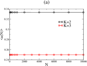
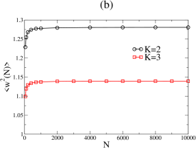
Figure 2.15: The steady-state observables in $K$-random network. (a) utilization as a function of system size. (b) width as a function of system size.

However, we were inspired by [64] to change the communication topology of the PEs by introducing random links in addition to the necessary short-range connections. In the next chapter we present our modification to the original conservative scheme on regular lattices to achieve a fully scalable algorithm where both scalability conditions are satisfied.

Chapter 3 SYNCHRONIZATION IN SMALL-WORLD NETWORKS

The divergent width of the synchronization landscapes in regular networks for very large systems, as discussed in the previous chapter, is the result of the divergent lateral correlation length $\xi$ of the virtual time surface reaching the system size $N$ in the steady-state [73, 79, 80, 81, 82]. To de-correlate the simulated time horizon, first, we modify the virtual communication topology of the PEs. The resulting communication network must include the original short-range (nearest-neighbor) connections to faithfully simulate the dynamics of the underlying system. In the modified network, the connectivity of the nodes (the number of links of a node) should remain non-extensive (i.e., only a finite number of virtual neighbors per node is allowed). This is in accordance with our desire to design a PDES scheme where no global intervention or synchronization is employed (PEs can only have $O(1)$ communication exchanges per step). It is clear that the added synchronization links (or at least some of them) have to be long range. Short range links alone would not change the universality class and the scaling properties of the width of the time horizon. One can satisfy this condition by selecting the additional links (called small-world links) randomly among all the nodes in the network. Also, fluctuations in the individual connectivity should be avoided for load balancing purposes, i.e., requiring the same number of added links (e.g., one) for each node is a reasonable constraint.

One may wonder how the collective behavior of the PDES scheme would change if each node was connected to the one located at the “maximum” possible distance away from it ($N/2$ on a ring) [Fig. 3.1(a)].

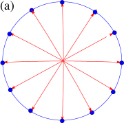
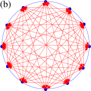
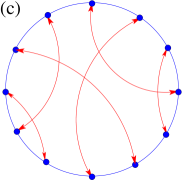
Figure 3.1: (a) Maximal-distance network in 1D where each node is connected to nearest neighboring nodes and to the node which is at the maximum distance. (b) Fully connected network where each node is connected to every other node in the network. (c) Small-world (SW) synchronization network in 1D, where each node is connected to a randomly chosen one in addition to the nearest neighbors.

Consider a linear coarse-grained Langevin equation with Gaussian noise where the effective strength of the added long-range links is $\gamma$,

$$\partial_{t}\tau_{i}(t)=(\tau_{i+1}+\tau_{i-1}-2\tau_{i})-\gamma(\tau_{i}-\tau_{i+N/2})+\eta_{i}(t)\;,$$ (3.1)

with periodic boundary conditions. Since Eq. (3.1) is translationally invariant, Fourier transformation decouples the equations for different wave numbers $k$ and one obtains for the steady-state structure factor (see Appendix A)

$$S(k)=\frac{D}{2[1-\cos(k)]+\gamma[1-\cos(kN/2)]}\;,$$ (3.2)

where $k=(2\pi n)/N$, $n=0,1,2,\ldots,N\!\!-\!\!1$ as before (and N is even for simplicity). Then for the average width we find

$$\langle w^{2}\rangle=\frac{1}{N}\sum_{k\neq 0}S(k)=\frac{1}{N}\sum_{k\neq 0}\frac{D}{2[1-\cos(k)]+\gamma[1-\cos(kN/2)]}\;.$$ (3.3)

Separating the terms with even and odd $n$ values above, we find

$$\langle w^{2}\rangle = \frac{1}{N}\sum_{n={\rm odd}}\frac{D}{2[1-\cos(2\pi n/N)]+2\gamma}$$ (3.4)

$$+ \frac{1}{N}\sum_{n={\rm even}}\frac{D}{2[1-\cos(2\pi n/N)]}\;.$$

The first sum yields a finite $N$-independent value in the $N$$\to$$\infty$ limit. The second sum, on the other hand, is identical to the width of the EW model on a regular network of size $N/2$. Thus, in the large $N$ limit the width for the “maximal-distance” connected network [Fig. 3.1(a)] diverges as $\langle w^{2}(N)\rangle$$\simeq$$DN/24$. Indeed, one can realize, that such regularly patterned long-range links make the network equivalent to a $2$$\times$$(N/2)$ quasi one-dimensional system with only nearest-neighbor interactions and helical boundary conditions. The above extreme case suggests, that the maximal-distance synchronization network cannot work either.

Now instead, consider the scenario where each node is connected to every other node in the network by a “weak” link, i.e., constructing a “fully” connected network as shown in Fig. 3.1(b). In this case we can rewrite the Langevin equation in Eq. (3.1) by using an effective strength of links, $\gamma/N$,

$$\partial_{t}\tau_{i}(t)=(\tau_{i+1}+\tau_{i-1}-2\tau_{i})-\frac{\gamma}{N}\sum_{j=1}^{N}(\tau_{i}-\tau_{j})+\eta_{i}(t)\;.$$ (3.5)

Performing the summation above yields an exact mean-field-like coupling, where each node is coupled to the average height:

$$\partial_{t}\tau_{i}(t)=(\tau_{i+1}+\tau_{i-1}-2\tau_{i})-\gamma(\tau_{i}-\bar{\tau})+\eta_{i}(t)\;,$$ (3.6)

where $\bar{\tau}=\sum_{j=1}^{N}\tau_{j}$ is the average height. For the steady-state structure factor one finds (see Appendix A)

$$S(k)=\frac{D}{2[1-\cos(k)]+\gamma}\;.$$ (3.7)

Then by using the relation between the structure factor and the width [Eq. 3.3] one obtains

$$\langle w^{2}\rangle=\frac{1}{N}\sum_{k\neq 0}S(k)=\frac{1}{N}\sum_{k\neq 0}\frac{D}{2[1-\cos(k)]+\gamma}\simeq\int_{-\infty}^{\infty}\frac{dk}{2\pi}\frac{D}{k^{2}+\gamma}=\frac{D}{2\sqrt{\gamma}}\;.$$ (3.8)

The above relation between the mean-field coupling constant $\gamma$ and the width shows that for a non-zero $\gamma$ the width is finite in the thermodynamic limit. But connecting each node in PDES to every other node would be cost-inefficient and cumbersome in terms of communication times. As we discuss in the next section, one can construct an “effectively” fully connected and yet cost-efficient network which has a finite width and relatively high progress rate by only employing a few random links.

3.1 One-Dimensional Small-World-Connected Synchronization Network

As we have seen in Chapter 2 our attempts to make the PDES fully scalable have failed because the PDES on short-range network is not measurement scalable (width is infinite for an infinite system). One of the proposed networks discussed in the previous section, the maximal-distance network, fails as a candidate for a fully scalable synchronization scheme because it is effectively equivalent to a short-range network. On the other hand, the fully connected network, is very inefficient in performance although it is measurement scalable. Motivated by the social networks we propose a network topology in which each node is connected to exactly one another randomly chosen node in addition to the nearest neighbors, resulting in a SW-like synchronization network. As we shall see, adding one random link to every node is cost-efficient and makes the network an “effectively” fully-connected one.

One of the basic structural characteristics of SW-like networks is the “low degree of separation” between the nodes. The most commonly used observables to analyze this property are the average shortest path length, $\delta_{avg}(N)$, and the maximum shortest path length, $\delta_{max}(N)$. The shortest path length between two nodes is defined as the minimum number of nodes one has to visit in order to go from one of the nodes to the other. The average shortest path length is the average of all these possible shortest paths between the nodes in the network. The maximum shortest path length, also known as diameter of the network, is the length of the longest among the shortest paths in the network. Both of these observables scale logarithmically with the system-size $N$ in SW-like networks [96]. The system-size dependence of these path lengths for our one-dimensional SW network, in which we have both nearest neighbors and random SW links, is logarithmic as expected, see Fig. 3.2(a)-(b).

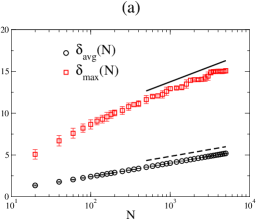
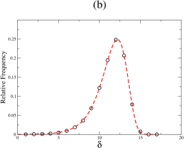
Figure 3.2: (a) Average and maximum shortest path lengths as a function of the number of nodes for the SW synchronization network in 1D, as described in the text. The latter is also referred to as the diameter of the network. The solid and dashed lines both indicate the logarithmic dependence. Note the normal-log axes. (b) Histogram for the length of the shortest paths in one realization of the network with system size $N$$=$$10^{4}$. The dashed curve is appropriately fitted Gumbel distribution for minima in the form $f(\delta)=\frac{1}{b}e^{\frac{\delta-a}{b}-e^{\frac{\delta-a}{b}}}$ where $a$$\cong$$12.2$ and $b$$\cong$$1.48$.

We now describe the modified algorithmic steps for the SW-connected PEs [8]. In the PDES on SW synchronization network, in every parallel time step each PE with probability $p$ compares its local simulated time with its full virtual neighborhood, and can only advance if it is the minimum in this neighborhood, i.e., if $\tau_{i}(t)\leq\min\{\tau_{i-1}(t),\tau_{i+1}(t),\tau_{r(i)}(t)\}$, where $r(i)$ is the random connection of PE $i$. With probability $(1-p)$ each PE follows the original scheme, i.e., the PE then can advance if $\tau_{i}(t)\leq\min\{\tau_{i-1}(t),\tau_{i+1}(t)\}$. Our network model including the nearest neighbors and random SW links can be seen in Fig. 3.1(c). Note that the occasional extra checking of the simulated time of the random neighbor is not needed for the faithfulness of the simulation. It is merely introduced to control the width of the time horizon. The occasional checking of the virtual time of the random neighbor (with rate $p$) introduces an effective strength $J=J(p)$ for these links. Note that this is a dynamic “averaging” process controlled by the parameter $p$ and can possibly be affected by nonlinearities in the dynamics through renormalization effects. The exact form of $J(p)$ is not known. The only plausible properties we assume for $J$ is that it is a monotonically increasing function of $p$ and is only zero when $p$=$0$.

In what follows, we focus on the characteristics of the dynamics on the network. As we have seen for the one-dimensional ring, the communication protocol between the nodes (up to linear terms) leads to simple relaxation, governed by the Laplacian on the regular grid. Random communication links give rise to analogous effective couplings between the nodes, corresponding to the Laplacian on the random part of the network. Thus, the large-scale properties of the virtual time horizon of our SW scheme are governed by the effective Langevin equation

$$\partial_{t}\hat{\tau}_{i}=\nabla^{2}\hat{\tau}_{i}-\sum_{j}J_{ij}(\hat{\tau}_{i}-\hat{\tau}_{j})+...+\eta_{i}(t)\;,$$ (3.9)

where the … stands for infinitely many non-linear terms (involving non-linear interactions through the random links as well), and $J_{ij}$ is proportional to the symmetric adjacency matrix of the random part of the network: $J_{ij}$$=$$J(p)$ if sites $i$ and $j$ are connected by a random link and $J_{ij}$$=$$0$ otherwise. For our specific SW construction each node has exactly one random neighbor, i.e., there are no fluctuations in the individual connectivity (degree) of the nodes. Our simulations (to be discussed below) indicate that when considering the large-scale properties of the systems, the Laplacian on the random part of the network generates an effective coupling $\gamma$ to the mean [8]. At the level of the structure factor, it corresponds to an effective mass $\gamma$ (in a field-theory sense)

$$S(k)\propto\frac{1}{\gamma+k^{2}}\;,$$ (3.10)

where $\gamma$$=$$\gamma(p)$ is a monotonically increasing function of $p$ with $\gamma(0)$=$0$.

We emphasize that the above is not a derivation of Eq. (3.10), but rather a “phenomenological” description of our findings. It is also strongly supported by exact asymptotic results for the (linear) EW model on SW networks, where the effect of the Laplacian on the random part of the network is to generate a mass [27, 29]. The averaging over the quenched network ensemble, however, can introduce nontrivial scaling and corrections in the effective coupling [27, 28, 29]. In our case, this is further complicated by the nonlinear nature of the interaction. The results of “simulating the simulation”, however, suggest that the dynamic control of the link strength and nonlinearities only give rise to a renormalized coupling and a corresponding renormalized mass. Thus, the dynamics of the BCS scheme with random couplings is effectively governed by the EW relaxation in a small-world [27, 29, 28]. From Eq. (3.10) it directly follows that the lateral correlation length in the infinite system-size limit

$$\xi\sim\gamma^{-1/2}\;,$$ (3.11)

i.e., becomes finite for all $p\not$=$0$ [Fig. 2.3(b)]. The presence of the effective mass term in the structure factor Eq. (3.10) implies that $\lim_{k\rightarrow 0}S(k)<\infty$, that is, there are no large amplitude long-wavelength modes in the surface. Consequently, the width $\langle w^{2}\rangle=(1/N)\sum_{k\not=0}S(k)$ is also finite. Our simulated time landscapes indeed show that they become macroscopically smooth when SW links are employed [Fig. 2.3(b)], compared to the the same dynamics with only short-range links [Fig. 2.3(a)].

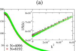
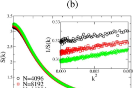
Figure 3.3: Structure factor for the 1D SW synchronization scheme with (a) $p$=$0.1$ and (b) $p$=$1$. The insets show $1/S(k)$ vs. $k^{2}$ for small values of $k$, confirming the coarse-grained prediction Eq. (3.10).

In the simulations, we typically performed averages over 10-100 network realizations, and compared the results to those of individual ones. Our results indicate that the observables we studied (the width and its distribution, the structure factor, and the utilization) display strong self-averaging properties, i.e., for large enough systems, they become independent of the particular realization of the

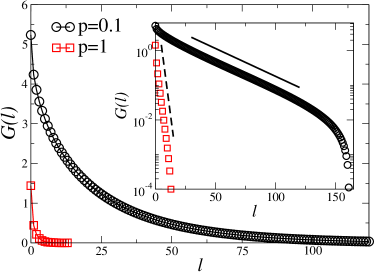
Figure 3.4: The spatial two-point correlation function as a function of the Euclidean distance $l$ between the nodes for two different values of $p$, indicating an exponential decay with an average correlation length $\xi$$\approx$$27$ and $\xi$$\approx$$1.6$ for $p$=$0.1$ and $p$=$1.0$, respectively. The number of nodes is $N$$=$$16$,$384$. The inset shows the same data in log-normal scale.

underlying SW network. Simulation results for the structure factor, $S(k)$, for the SW synchronization scheme are shown in Fig. 3.3(a) and (b). If an infinitesimally small $p$ is chosen, $S(k)$ approaches a finite constant in the limit of $k$$\rightarrow$$0$, and in turn, the virtual time horizon becomes macroscopically smooth with a finite width.

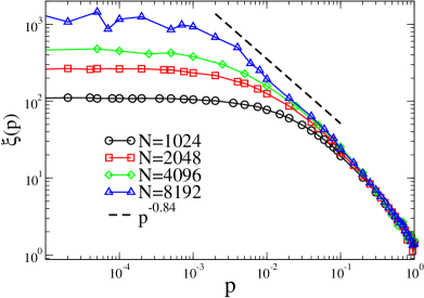
Figure 3.5: Correlation length ($\xi$) vs. $p$ for different system-sizes. The dashed line corresponds to the estimate of the exponent $s$, $\xi(p)\sim p^{-s}$ with $s$$\approx$$0.84$, in the small-$p$ regime for an asymptotically infinite system.

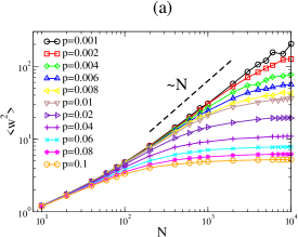
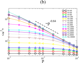
Figure 3.6: (a) The average steady-state width in the 1D SW synchronization landscape as a function of the system size for different values of $p$ in the range of $[10^{-3},10^{-1}]$. The dashed line indicates the EW/KPZ scaling, corresponding to the small system-size behavior. (b) The average steady-state width in the 1D SW synchronization landscape as a function of $p$ for different values of $N$ in the range of $[40,10^{4}]$. The dashed line indicates the best-fit power law in the asymptotic large-$N$ small-$p$ regime to extract the correlation length exponent $s$, according to Eqs. (3.12)-(3.14).

A possible (phenomenological) way to obtain the correlation length is to fit our structure factor data to Eq. (3.10), more specifically, by plotting $1/S(k)$ versus $k^{2}$, which exhibits a linear relationship. By a linear fit, $\gamma$ is then the ratio of the intercept and the slope (insets in Fig. 3.3). Alternatively, one can confirm that the

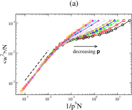
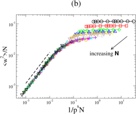
Figure 3.7: The scaled versions of Fig. 3.6(a) and (b), as proposed by Eq. (3.12) and Eq. (3.14) by plotting $\left\langle w^{2}\right\rangle/N$ vs. $1/p^{s}N$ with $s$=$0.84$. The data points are identical in (a) and (b), but data points connected by a line have the same value of $p$ in (a) and have the same value of $N$ in (b), as obtained by rescaling Fig. 3.6(b) and (b), respectively. The dashed line corresponds to the asymptotic small-$x$ behavior of the scaling function $g(x)$ [Eq. (3.13)].

massive propagator Eq. (3.10) indeed leads to an exponential decay in the two-point correlation function from which the correlation length can also be extracted [Fig. 3.4]. In our case with a system-size $N$=$16$,$384$, $\xi$$\approx$$27$ for $p$=$0.1$ and $\xi$$\approx$$1.6$ for $p$=$1$. Figure 3.5(c) shows the correlation length extracted from the structure factor $S(k)$ as a function of $p$ for different system-sizes.

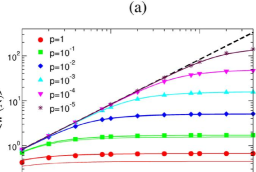
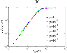
Figure 3.8: (a) Steady-state width for linear EW model as a function of the system-size from [28] for comparison. The solid lines from are from theoretical calculations and the symbols from simulations. The dashed line shows the behavior of the width when there is no SW links, namely the BCS scheme (short-range network) (b) The scaled version of (a) by using Eq. (3.12) and Eq. (3.13). For the linear EW model the scaling does not have any noticeable corrections.

An alternative way to determine the correlation length is using the finite-size scaling of the width $\langle w^{2}\rangle$. From dimensional analysis it follows that $\langle w^{2}\rangle$ has length dimension in 1D. There are two length scales in the system: the linear system size $N$ and the correlation length $\xi$ of an infinite system. For $p=0$, $\langle w^{2}\rangle$$\sim$$N$, while for $p$$>$$0$ and $N$$\to$$\infty$, $\langle w^{2}\rangle$$\sim$$\xi$. For non-zero $p$ and finite $N$ the scaling of the steady-state width can be expected [28] to follow

$$\left\langle w^{2}\right\rangle=Ng(\xi/N)\;,$$ (3.12)

where $g(x)$ is a scaling function such that

$$g(x)\sim\left\{\begin{array}[]{ll}x&\mbox{if $x$$\ll$$1$}\\ \mbox{const.}&\mbox{if $x$$\gg$$1$}\end{array}\right.\;.$$ (3.13)

For non-zero $p$ and for sufficiently small systems ($N$$\ll$$\xi(p)$) one can confirm that the behavior of the width follows that of the system without random links $\langle w^{2}\rangle$$\sim$$N$ [Fig. 3.6(a)]. For large-enough systems, on the other hand, we can extract the $p$-dependence of the infinite-system correlation length as $\langle w^{2}\rangle$$\sim$ $\xi(p)$ [Fig. 3.6(b)], yielding

$$\xi(p)\sim p^{-s}\;,$$ (3.14)

where $s$$\approx$$0.84$.

We then studied the data collapse as proposed by Eq. (3.12) by plotting $\langle w^{2}\rangle/N$ vs. $1/p^{s}N$. In fact, we performed this rescaling originating from both raw data sets Fig. 3.6(a) and (b). The resulting scaled data points in Fig. 3.7(a) and (b), of course, are identical in the two figures, but the lines connect data points with the same value of $p$ in Fig. 3.7(a) and with the same value of $N$ in Fig. 3.7(b). These scaled plots in Fig. 3.7 indicate that there are very strong corrections to scaling: data for larger $p$ or smaller $N$ values “peel off” from the proposed scaling form in Eq. (3.13) relatively quickly. These strong corrections are possibly the result of the nonlinear nature of the interaction between the nodes on the quenched network. We note that the linear EW model on identical networks exhibits the scaling proposed in Eq. (3.12) and Eq. (3.13) without noticeable corrections [28] [Fig. 3.8(a) and (b)].

The non-zero $\gamma$, leading to a finite correlation length, $\xi$, ensures a finite width in the infinite system-size limit. Our simulations show that the width saturates to a finite value for $p$$>$$0$ [Fig. 3.9(a)].

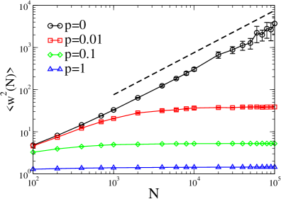
Figure 3.9: The steady-state width as a function of system size for 1D SW synchronization network as a function of system size. The width saturates to finite values as long as $p\not=0$. The dashed line shows the power-law divergence for BCS in 1D. Note the log-log scales.

The distribution of the width $P(w^{2})$ changes from the EW/KPZ distribution to a delta function for non-zero values of $p$ as the system size goes to infinity. Figure 3.10(a) and (b) shows the width distributions for $p$=$0.1$ and $p$=$1$, respectively. The scaled width distributions (to zero mean and unit variance), however, exhibit the convergence to a delta function through nontrivial shapes for different values of $p$. For $p$=$0.1$

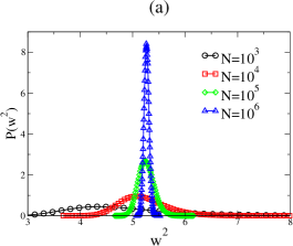
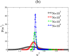
Figure 3.10: Steady-state width distributions in the 1D SW synchronization scheme for (b) $p$=$0.1$ and for (c) $p$=$1.0$. The distributions were constructed using ten different network realizations, except for $N$=$10^{6}$, where only one realization was obtained due to computational limitations. All width distributions, however, indicated self-averaging.

[Fig. 3.11(a)] the distributions appear to slowly converge to a Gaussian as the system-size increases. For $p$=$1$ [Fig. 3.11(b)], the trend is opposite up to the system sizes we could simulate; as the system-size increases, the distributions exhibit progressively non-Gaussian features (closer to an exponential) around the center up to $N$=$10^{6}$. Note that not only the average width $\langle w^{2}\rangle$, but also the full distribution $P(w^{2})$ is self-averaging, i.e., is independent of the particular realization of the underlying SW network.

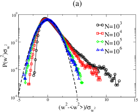
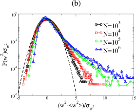
Figure 3.11: Steady-state width distributions for the 1D SW synchronization scheme scaled to zero mean and unit variance for (a) $p$=$0.1$ and (b) $p$=$1.0$. The dashed curves are similarly scaled Gaussians for comparison.

To get some insight into the possible role of the disorder in approaching the limit distribution of the width, we studied the two-point function for individual pair of nodes. Note, that by construction, the observable previously considered, $G(l)$, is the site (or spatially) averaged two-point function over all nodes with Euclidean distance $l$, $G(l)$$=$$\frac{1}{N}\sum_{i=1}^{N}\langle(\tau_{i}-\bar{\tau})(\tau_{i+l}-\bar{\tau})\rangle$. If the height values on the nodes for a fixed network realization are sufficiently weakly correlated, the width distribution should converge to a Gaussian, governed by the central limit theorem [97, 98]. As we saw above, for larger values of $p$, this may not be the case, at least for finite systems.

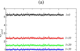
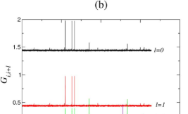
Figure 3.12: Two-point correlation function for each node $i$ for various separation $l$ for a fixed 1D SW synchronization network with size $N$$=$$16,384$ (a) $p$$=$$0.1$ and (b) $p$$=$$1$. The horizontal lines correspond to spatial average $G(l)$ for each $l$.

In order to have some measure how the individual terms in the width are correlated, $w^{2}$$=$$(1/N)\sum_{i=1}^{N}(\tau_{i}-\bar{\tau})^{2}$, we constructed the two-point function for all sites $i$ for a few chosen separation $l$ [Fig. 3.12] for a fixed network realization. Of course, as already discussed, averaging over all $i$, will yield an exponential decay as a function of $l$. Now, instead, we focus on the full two-point correlation “profile” for a given separation $l$. As can be seen in Fig. 3.12(a), for $p$$=$$0.1$, the node-to-node fluctuations in the two-point correlation profile, compared to their spatial average $G(l)$, are small. With the increasing strength of the disorder ($p$$=$$1$), however, certain sites develop abnormally large, frozen correlations as shown in Fig. 3.12(b). The deviation of the two-point correlations for these few nodes, from the mean $G(l)$, is much larger than those for the other nodes, and is comparable to the mean itself. This property can work “against” the necessary conditions of the central limit theorem and, thus, can have a strong effect on the convergence (or the apparent lack of it) of the width distribution to a Gaussian.

The effect of the random communication links on the utilization can be understood as follows. According to the algorithmic rules, the virtual times of the full network neighborhood (including the random neighbor) are checked with probability $p$, while with probability $(1$$-$$p)$ only short-ranged synchronization is employed. Thus, the average progress rate of the simulated times becomes

$$\langle u\rangle=(1-p)\langle\Theta(-\phi_{i-1})\Theta(\phi_{i})\rangle+p\langle\Theta(-\phi_{i-1})\Theta(\phi_{i})\Theta(\tau_{r(i)}-\tau_{i})\rangle\;.$$ (3.15)

Note that the disorder (network) averaging makes the right hand side independent of $i$. In the presence of the SW links the regular density of local minima $\langle\Theta(-\phi_{i-1})\Theta(\phi_{i})\rangle$ remains nonzero (in fact, increases compared to the short-range synchronized BCS scheme) [8, 87, 99]. Thus, for an infinitesimally small $p$, the utilization, at most, can be reduced by an infinitesimal amount, and the SW-synchronized simulation scheme maintains a nonzero average progress rate. This is favorable in PDES where global performance requires both finite width and nonzero utilization. With the SW synchronization scheme, both of these objectives can be achieved. For example, for $p$$=$$0.1$ $\langle u(\infty)\rangle\simeq 0.242$, while for $p$$=$$1.0$ $\langle u(\infty)\rangle\simeq 0.141$. The steady-state utilization as a function of system size for various values of $p$ can be seen in Fig. 3.13.

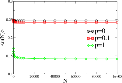
Figure 3.13: Steady-state utilization of SW synchronization network in 1D as a function of system-size for three different values of $p$$=$$0$ (BCS), $p$$=$$0.1$ and $p$$=$$1$.

3.2 Two-dimensional Small-World-Connected Synchronization Network

The de-synchronization (roughening of the virtual time horizon) again motivates the introduction of the possibly long-range, quenched random communication links on top of the 2D regular network. Each node will have exactly one (bi-directional) random link as illustrated in Fig. 2.9(b). The actual “microscopic” rules are analogous to the 1D SW case: with probability $p$ each node will check the local simulated times of all of its neighbors, including the random one, and can increment its local simulated time by an exponentially distributed random amount only if it is a “local” minimum (among the four nearest neighbors and its random neighbor). With probability $(1$$-$$p)$, only the four regular lattice neighbors are checked for the local minimum condition.

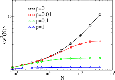
Figure 3.14: (a) The average steady-state width as a function of linear system size for different $p$ values in the 2D SW synchronization scheme. The data for $p$=$0$ corresponds to the 2D BCS scheme on a regular network with only nearest-neighbor connections.

The effect of the synchronization through the random links is, again, to stop kinetic roughening and to suppress fluctuations in the synchronization landscapes. Contour plots of the synchronization landscapes are shown in Fig. 2.10(b) and (c) for $p$$=$$0.1$ and $p$$=$$1$, respectively. Our results indicate that for any nonzero $p$ the

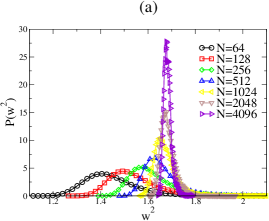
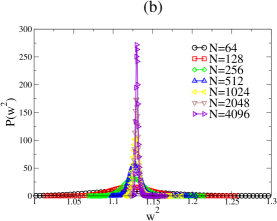
Figure 3.15: Steady-state width distributions in the 2D SW synchronization scheme for (a) $p$$=$$0.1$ and for (b) $p$$=$$1.0$ for various system sizes.

width of the surface approaches a finite value in the limit of $N$$\to$$\infty$ [Fig. 3.14(a)]. At the same time, the distribution approaches a delta-function in the large system-size limit as shown in Fig. 3.15(a) and (b). The scaled distributions (to zero mean and unit variance) again show that at least for the finite systems we observed, the shape of these distribution differs from a Gaussian [Fig. 3.16(a) and (b)]. The deviation from the Gaussian around the center of the distribution is stronger for a larger value of $p$ where the influence of the quenched random links are stronger. Note that for the 1D SW landscapes as well, the width distribution only displayed a crossover to Gaussian behavior for smaller values of $p$ and for very large linear system sizes ($N>{\cal O}(10^{4})$. In the 2D SW case, these linear system sizes are computationally not achievable, and the convergence to a Gaussian width distribution remains an open question.

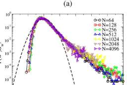
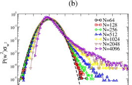
Figure 3.16: Steady-state width distributions in the 2D SW synchronization scheme scaled to zero mean and unit variance for (a) $p$$=$$0.1$ and for (b) $p$$=$$1.0$. The dashed curves are similarly scaled Gaussians for comparison.

The underlying reason for the finite width is again a finite average correlation length between the nodes. The 2D structure factor exhibits a massive behavior, i.e., $S(|{\bf k}|)$ approaches a finite value in the limit of k$\to$0 [Fig. 3.17(a) and (b)]. For small wave numbers, the approximate behavior of the structure factor is again $S(|{\bf k}|)\propto 1/(|{\bf k}|^{2}+\gamma)$ as can be seen in the inset of Fig. 3.17(b), with strong finite-size corrections to $\gamma$. The relevant feature of the synchronization dynamics on a SW network is the generation of the effective mass $\gamma$. Nonlinearities can give rise to a renormalized mass, but the relevant operator is the Laplacian on the random part of the network.

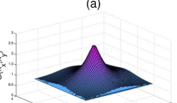
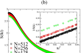
Figure 3.17: (a) Steady-state structure factor for the 2D SW scheme as a function of the wave-vector components $k_{x}$ and $k_{y}$ for $p$$=$$1.0$. (b) Structure factor as a function of magnitude of the wave vector, $|\textbf{k}|$, for the 2D SW synchronization scheme for $p$=$1.0$. The inset shows $1/S(\textbf{k})$ vs. $|\textbf{k}|^{2}$ for small values of $|\textbf{k}|$.

In the 2D SW synchronization scheme the steady-state utilization is smaller than its purely 2D counterpart (BCS in 2D), as a result of the possible additional checking with the random neighbors. For small values of $p$, however, it is reduced only by a small amount, and remains nonzero in the limit of an infinite number of nodes [Fig. 3.18]. For example, for $p$$=$$0.1$ $\langle u\rangle_{\infty}$$\simeq$$0.1198$, while for $p$=$1$ $\langle u\rangle_{\infty}$$\simeq$$0.084$.

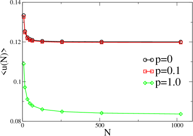
Figure 3.18: Steady-state utilization of SW synchronization network in 2D as a function of system-size for three different values of $p$$=$$0$ (BCS), $0.1$ and $1$.

3.3 Synchronization in scale-free networks

The Internet is a spontaneously grown collection of connected computers. The number of (only) webservers by February 2003 reached over 35 million [100]. The number of PC-s in use (Internet users) surpassed 660 million in 2002, and it is projected to surpass one billion by 2007 [101]. The idea for using it as a giant supercomputer is rather natural: many computers are in an idle state, running at best some kind of screen-saver software, and the “wasted” computational time is simply immense. Projects such as SETI@home or the GRID consortium [17] are targeting to harness the power lost in screen-savers.

Most of the problems solved currently with distributed computation on the Internet are “embarrassingly parallel” [16] , i.e., the computed tasks have little or no connection to each other similar to starting the same run with a number of different random seeds, and at the end collecting the data to perform statistical averages. However, before complex problems can be solved in real time on the Internet a number of challenges have to be solved, such as the task allocation problem which is rather complex by itself [66].

Here one can ask the following question: Given that task allocation is resolved and the PE communication topology on the internet is a scale-free network, what are the scalability properties of a conservative synchronization scheme on such networks? Here we present numerical results, for the conservative PDES scheme, as measured on a model of scale-free networks, namely the Barabási-Albert model (BA) [5, 102]. This network is created through the stochastic process of preferential attachment: to the existing network at time $t$ of $N$ nodes, attaches the $N$$+$$1^{st}$ node with $m$ links (“stubs”) at time $t$$+$$1$, such that each stub attaches to a node with probability proportional to the existing degree of the node. Here we will only present the $m$$=$$1$ case, when the network is a scale-free tree. Once we reach a given number of nodes in the network, we stop the process and use the random network instance to simulate the synchronization, using the evolution equation [Eq. (2.1)) for the time horizon. While in case of regular topologies, the degree of a node is constant, e.g. for $d$-dimensional “square” lattices, $P^{(N^{d})}(k)=2d\delta_{k,2d}$ , for the BA network, it is a power law in the asymptotic ($N$$\to$$\infty$) limit : $P^{BA}(k)\simeq 2m^{2}k^{-3}$. The condition for a site to be updated, i.e., that its virtual time is a local minimum, is a local property, and thus we expect that the utilization itself be correlated with local structural properties of the graph, such as the degree distribution. Figure 3.19 shows the steady state ($t$$\to$$\infty$, on a fixed BA network of $N$ nodes) values of the average utilization as function of the network size $N$. Notice that strictly speaking, the conservative PDES scheme is computationally non-scalable. An empirical fit suggest that $\langle u(N)\rangle=\langle u(N,t$$=$$\infty)\rangle\simeq\left[\ln{\left(aN^{b}\right)}\right]^{-1}$ with $a\simeq 3.322$ and $b=0.902$, i.e., the computation is only logarithmically (or marginally) non-scalable. For a system of $N$$=$$10^{3}$ nodes we have found a steady state utilization (for the worst case scenario) of $\langle u\rangle$$=$$0.1328$ ($13.3\%$ efficiency), while for a system of a million nodes, $N$$=$$10^{6}$, the utilization dropped only to $\langle u\rangle$$=$$0.073$ ($7.3\%$ efficiency), by less than half of its value. For practical purposes the conservative PDES scheme can be considered computationally scalable, and this type of non-scalability we will call logarithmic (or marginal) non-scalability.

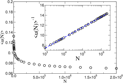
Figure 3.19: Steady-state utilization for the scale-free BA network

Figure 3.20 shows the scaling of the width of the fluctuations for the time horizon as function of time, and the scaling of its value in the steady-state as function of system size (inset). Notice, that while the steady state width diverges to infinity, it only does so logarithmically, $\langle w^{2}(N,t$$=$$\infty)\rangle\simeq\left[\ln{\left(cN^{d}\right)}\right]$ with $c$$\simeq$$1.25$ and $d$$\simeq$$0.401$. Some specific values: $\langle w^{2}(10^{3},t$$=$$\infty)\rangle\simeq 3.01$, $\langle w^{2}(10^{5},t$$=$$\infty)\rangle$$\simeq$$4.78$. This means that the measurement phase of the conservative PDES scheme on a scale-free network is non-scalable either, however, it is so only logarithmically, and for practical purposes the scheme can be considered scalable. Overall, the conservative PDES scheme has logarithmic (or marginal) non-scalability on scale-free networks.

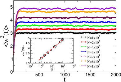
Figure 3.20: Behavior of the time horizon width for the scale-free BA network (scale-free tree with $m$$=$$1$). The inset shows the scaling of the steady-state width as a function of system size, $N$ (note the log-normal scale on the inset).

Chapter 4 EXTREME FLUCTUATIONS IN SMALL-WORLD NETWORKS

Large fluctuations in networks are to be avoided for many reasons such as scalability or stability. In the absence of global intervention or control, this can be a difficult task. Motivated by the results in Chapter III [8] for small-world (SW) [19] synchronized autonomous systems in the context of scalable parallel computing, we investigate the steady-state properties of the extreme fluctuations in SW-coupled interacting systems with relaxational dynamics [103, 104]. Since the introduction of SW networks [19] it has been well established that such networks can facilitate autonomous synchronization [36, 37, 105]. In addition to the average “load” in the network, knowing the typical size and the distribution of the extreme fluctuations [106, 107, 108] is of great importance from a system-design viewpoint, since failures and delays are triggered by extreme events occurring on an individual node.

Relationship between extremal statistics and universal fluctuations in correlated systems has been studied intensively [109, 110, 111, 112, 113, 114, 115, 116, 118, 119, 120, 121, 122, 123, 124, 125]. The focus of a number of these studies was to find connections, if any, between the probability distribution of global observables or order parameters (such as the width in surface growth problems [73] or the magnetization in magnetic systems [126]) and known universal extreme-value limit distributions [106, 107, 108]. Recent analytic results demonstrated [118, 121] that, in general (except for special cases [116, 117]), there are no such connections. Here we discuss to what extent SW couplings (extending the original dynamics through the random links) lead to the suppression of the extreme fluctuations of the local order parameter or field variable in various noisy environments. We illustrate our findings on the actual PDES synchronization problem in scalable parallel computing [8]. In Sec. 4.1 we review the well-known extreme-value limit distributions for exponential-like and power-law-tail distributed random variables. In Sec. 4.3 we discuss the results [103, 104] on the scaling behavior of the extreme fluctuations and their distribution. for the Edwards–Wilkinson model [86] on SW networks [27] with exponential-like noise. In Sec. 4.3 we apply these results to study the extreme load fluctuations in SW-synchronized PDES schemes [40, 41], applicable to high performance parallel architectures and large-scale grid-computing networks. In Sec. 4.4 we extend our studies [103, 104] and consider the synchronization problem in the presence of power-law tailed noise.

4.1 Extreme-Value Distributions for Independent Random Variables

4.1.1 Exponential-like variables

First, we consider the case when the individual complementary cumulative distribution $P_{>}(x)$ (the probability that the individual stochastic variable is greater than $x$) decays faster than any power law, i.e., exhibits an exponential-like tail in the asymptotic large-$x$ limit. (Note that in this case the corresponding probability density function displays the same exponential-like asymptotic tail behavior.) We will assume $P_{>}(x)\simeq e^{-cx^{\delta}}$ for large $x$ values, where $c$ and $\delta$ are constants. Then the cumulative distribution $P_{<}^{\max}(x)$ for the largest of the $N$ events (the probability that the maximum value is less than $x$) can be approximated as [122, 127, 128]

$$P_{<}^{\max}(x)=[P_{<}(x)]^{N}=[1-P_{>}(x)]^{N}=e^{N\ln[1-P_{>}(x)]}\simeq e^{-NP_{>}(x)}\;,$$ (4.1)

where one typically assumes that the dominant contribution to the statistics of the extremes comes from the tail of the individual distribution $P_{>}(x)$. With the exponential-like tail in the individual distribution, this yields

$$P_{<}^{\max}(x)\simeq e^{-e^{-cx^{\delta}+\ln(N)}}.$$ (4.2)

The extreme-value limit theorem states that there exists a sequence of scaled variables $\tilde{x}=(x-a_{N})/b_{N}$, such that in the limit of $N$$\to$$\infty$, the extreme-value probability distribution for $\tilde{x}$ asymptotically approaches the Fisher–Tippett–Gumbel (FTG) distribution [106, 107]:

$$\tilde{P}_{<}^{\max}(\tilde{x})\simeq e^{-e^{-\tilde{x}}}\;,$$ (4.3)

with mean $\langle\tilde{x}\rangle$$=$$\gamma$$=$$0.577\ldots$ (Euler constant) and variance $\sigma_{\tilde{x}}^{2}=$ $\langle\tilde{x}^{2}\rangle$$-$$\langle\tilde{x}\rangle^{2}$ $=\pi^{2}/6$. From Eq. (4.2), one can deduce [128] that to leading order the scaling coefficients are $a_{N}=\left[\frac{\ln(N)}{c}\right]^{1/\delta}$ and $b_{N}=(\delta c)^{-1}\left[\frac{\ln(N)}{c}\right]^{(1/\delta)-1}$. The average value of the largest of the $N$ original variables then scales as

$$\langle x_{\max}\rangle=a_{N}+b_{N}\gamma\simeq\left[\frac{\ln(N)}{c}\right]^{1/\delta}$$ (4.4)

(up to ${\cal O}(\frac{1}{\ln(N)})$ correction) in the asymptotic large-$N$ limit. When comparing with experimental or simulation data, instead of Eq. (4.3), it is often convenient to use the form of the FTG distribution which is scaled to zero mean and unit variance, yielding

$$\tilde{P}_{<}^{\max}(y)=e^{-e^{-(ay+\gamma)}}\;,$$ (4.5)

where $a=\pi/\sqrt{6}$ and $\gamma$ is the Euler constant. In particular, the corresponding FTG density then becomes

$$\tilde{p}^{\max}(y)=ae^{-(ay+\gamma)-e^{-(ay+\gamma)}}\;.$$ (4.6)

4.1.2 Power-law tailed variables

Now consider independent identically distributed random variables where the tail of the complementary cumulative distribution decays in a power law fashion, i.e., $P_{>}(x)\simeq A/x^{\mu}$ for large values of $x$. Assuming again that the dominant contribution to the statistics of the extremes comes from the tail of the individual distribution [122, 127, 128], Eq.(4.1) yields

$$P_{<}^{\max}(x)\simeq e^{-NP_{>}(x)}\simeq e^{-NA/x^{\mu}}\;.$$ (4.7)

Introducing the scaled variable $\tilde{x}=x/b_{N}$, where $b_{N}=(AN)^{1/\mu}$, yields the standard form of the so called Fréchet distribution for the extremes in the asymptotic large-$N$ limit [106, 108]

$$\tilde{P}_{<}^{\max}(\tilde{x})=e^{-1/\tilde{x}^{\mu}}\;,$$ (4.8)

and the corresponding probability density

$$\tilde{p}^{\max}(\tilde{x})=\frac{\mu}{\tilde{x}^{\mu+1}}e^{-1/\tilde{x}^{\mu}}\;.$$ (4.9)

One can note that the tail behavior of the extremes has been inherited from that of the original individual variables, i.e., $\tilde{p}^{\max}(\tilde{x})\sim 1/\tilde{x}^{\mu+1}$ for large values of $\tilde{x}$. The first moment of the extreme exist if $\mu>1$ and for the average value of the largest of the $N$ original power-law variables one finds

$$\langle x_{\max}\rangle=b_{N}\langle\tilde{x}\rangle\simeq\Gamma(1-1/\mu)(AN)^{1/\mu}\sim N^{1/\mu}\;$$ (4.10)

where $\Gamma(z)$ is Euler’s gamma function. For comparison with experimental or simulation data it is often convenient to use an alternative scaling for the extremes $y=x/\langle x_{\max}\rangle$, yielding collapsing ($N$-independent) probability density functions similar to Eq.(4.9)

$$\tilde{p}^{\max}(y)=\frac{\mu}{\Gamma^{\mu}(1-1/\mu)y^{\mu+1}}e^{-1/(\Gamma^{\mu}(1-1/\mu)y^{\mu})}\;.$$ (4.11)

4.2 Extreme Fluctuations in 1D BCS Network

We consider again the simplest stochastic model with linear relaxation on a SW network used in the previous chapter [Eq. (3.9)]. In this chapter in addition to the width, we will study the scaling behavior of the largest fluctuations (e.g., above the mean) in the steady-state

$$\langle\Delta_{\max}\rangle\equiv\langle\tau_{\max}-\bar{\tau}\rangle\;.$$ (4.12)

As discussed in Chapter 2 and 3, Eq. (3.9) (and its generalization with a KPZ-like nonlinearity [84]) governs the steady-state progress and scalability properties of a large class of PDES schemes [8, 39, 77, 79, 129]. In this context, the local height variables $\{\tau_{i}(t)\}_{i=1}^{N}$ correspond to the progress of the individual processors after $t$ parallel steps. The EW/KPZ-type relaxation at a coarse-grained level originates from the “microscopic” (node-to-node) synchronizational rules. In the absence of the random links with purely short-range connections, the corresponding steady-state landscape is rough [73] (de-synchronized state), i.e., it is dominated by large-amplitude long-wavelength fluctuations. The extreme values of the local fluctuations emerge through these long-wavelength modes and, in one dimension, the extreme and average fluctuations follow the same power-law divergence with the system size [79, 110, 124, 125, 129]

$$\langle\Delta_{\max}\rangle\sim w\sim N^{\alpha}\;,$$ (4.13)

where $\alpha$ is the roughness exponent [73] [Fig. 4.1(a)].

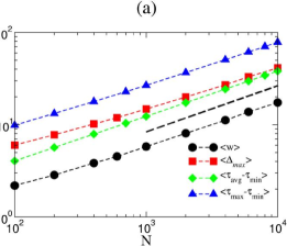
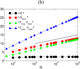
Figure 4.1: (a) Scaling behavior of the average ($w$) and the extreme (above the mean $\Delta_{\max}$, below the mean $\langle\bar{\tau}-\tau_{min}\rangle$, maximum spread $\langle\tau_{max}-\tau_{min}\rangle$) fluctuations in the virtual time horizon for the conservative PDES scheme in the steady state. The processors are connected in a ring-like fashion. Note the log-log scales. The dashed line represents the theoretical power law with the roughness exponent $\alpha$$=$$1/2$. (b) The same quantities as in (a), but the processors are connected by a small-world topology and the additional synchronization through the random link is performed with probability $p$$=$$0.10$ at every parallel step (log-normal scales). The solid straight line indicates the weak logarithmic increase of the extreme fluctuations with the system size.

The extreme-value limit theorems sketched in the previous section are valid only for independent (or short-range correlated) random variables. Since the heights are strongly correlated in the 1D BCS scheme, the known extreme-value limit theorems cannot be used. A recent work on this issue sheds some light on the distribution of the extreme heights in the 1D BCS [124, 125]. Equation (4.13) suggests that the normalized probability density function of the maximum relative

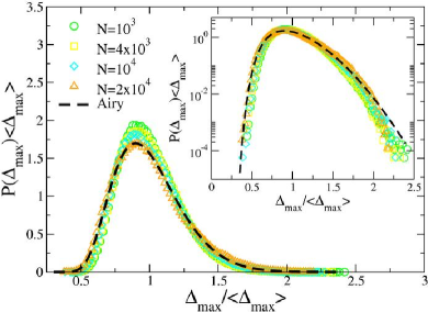
Figure 4.2: The scaled distributions of maximum relative height of the 1D BCS for different system-sizes. The dashed line is the Airy distribution function [124]. The inset is the log-normal version of the same data to show the agreement with the theoretical curve in the tail .

height $\Delta_{max}$ has a universal scaling form, $P(\Delta_{max},N)$$\sim$$N^{-\alpha}f(\Delta_{max}/N^{\alpha})$. For the 1D EW/KPZ with periodic boundary conditions ($\alpha$$=$$1/2$), by using path integral techniques [124] $f(x)$ was found to be the so-called Airy distribution function. Our simulation results show that the appropriately scaled maximum relative height distributions are in agreement with the theoretical distribution from [124] [Fig. 4.2].

4.3 Extreme Fluctuations in Small-World-Connected Network

The important feature of the EW model on SW networks is the development of an effective nonzero mass $\gamma(p)$, corresponding to an actual or pseudo gap in a field theory sense [27, 30, 130], generated by the quenched-random structure [27]. In turn, both the average correlation length $\xi\simeq[\gamma(p)]^{-1/2}$ and the width $w\simeq(1/\sqrt{2})[\gamma(p)]^{-1/4}$ approach a finite value (synchronized state) and become self-averaging in the $N$$\to$$\infty$ limit [99]. Thus, the average correlation length becomes finite for an arbitrarily small but nonzero strength of the random links (one such link per site). This is the fundamental effect of extending the original dynamics to a SW network: it decouples the fluctuations of the originally correlated system. Then, the extreme-value limit theorems can be applied using the number of independent blocks $N/\xi$ in the system [122, 128]. Further, if the tail of the noise distribution decays in an exponential-like fashion, the individual relative height distribution will also do so , and depends on the combination $\Delta_{i}/w$, where $\Delta_{i}=\tau_{i}$$-$$\bar{\tau}$ is the relative height measured from the mean at site $i$. Considering, e.g., the fluctuations above the mean for the individual sites, we will then have $P_{>}(\Delta_{i})\simeq\exp[-c(\Delta_{i}/w)^{\delta}]$, where $P_{>}(\Delta_{i})$ denotes the “disorder-averaged” (averaged over network realizations) single-site relative height distribution, which becomes independent of the site $i$ for SW networks. From the above it follows that the cumulative distribution for the extreme-height fluctuations relative to the mean $\Delta_{\max}$$=$$\tau_{\max}$$-$$\bar{\tau}$, if scaled appropriately, will be given by Eq. (4.3) [or alternatively by Eq. (4.5)] in the asymptotic large-$N$ limit (such that $N/\xi$$\gg$$1$). Further, from Eq. (4.4), the average maximum relative height will scale as

$$\langle\Delta_{\max}\rangle\simeq w\left[\frac{\ln(N/\xi)}{c}\right]^{1/\delta}\simeq\frac{w}{c^{1/\delta}}\left[\ln(N)\right]^{1/\delta}\;,$$ (4.14)

where we kept only the leading order term in $N$. Note, that both $w$ and $\xi$ approach their finite asymptotic $N$-independent values for SW-coupled systems. Also, the same logarithmic scaling with $N$ holds for the largest relative deviations below the mean $\langle\bar{\tau}$$-$$\tau_{\min}\rangle$ and for the maximum spread $\langle\tau_{\max}$$-$$\tau_{\min}\rangle$. This weak logarithmic divergence, which one can regard as marginal, ensures synchronization for practical purposes in SW coupled multi-component systems with local relaxation in an environment with exponential-like noise.

To study the extreme fluctuations of the SW-synchronized virtual time horizon, we “simulated the simulations”, i.e., the evolution of the local simulated times based on the above exact algorithmic rules [103]. By constructing histograms for $\Delta_{i}$, we observed that the tail of the disorder-averaged individual relative-height distribution decays exponentially ($\delta$$=$$1$) [Fig. 4.3].

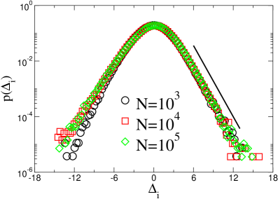
Figure 4.3: Disorder-averaged probability densities for the local height fluctuations for the SW-synchronized ($p$$=$$0.10$) landscape for three system sizes indicated in the figure. Note the log-normal scales. The solid straight line indicates the exponential tail.

Then, we constructed histograms for the extreme-height fluctuations Fig. 4.4(a).

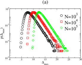
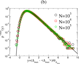
Figure 4.4: (a) Disorder-averaged probability distributions for the extreme height fluctuations for the SW-synchronized conservative PDES time horizons with $p$$=$$0.10$ for three system sizes indicated in the figure. Note the log-normal scales. (b) The same as (a), but the probability densities are scaled to zero mean and unit variance. The solid curve corresponds to the similarly scaled FTG density Eq. (4.6) for comparison.

The scaled histograms, together with the similarly scaled FTG density Eq. (4.6), are shown in Fig. 4.4(b). We also observed that the distribution of the extreme values becomes self-averaging, i.e., independent of the network realization. Figure 4.1(b) shows that for sufficiently large $N$ (such that $w$ essentially becomes system-size independent) the average (or typical) size of the extreme-height fluctuations diverge logarithmically, according to Eq. (4.14) with $\delta$$=$$1$. We also found that the largest relative deviations below the mean $\langle\bar{\tau}$$-$$\tau_{\min}\rangle$, and the maximum spread $\langle\tau_{\max}$$-$$\tau_{\min}\rangle$ follow the same scaling with the system size $N$ [Fig. 4.1(b)]. Note, that for our specific system (PDES time horizon), the “microscopic” dynamics is inherently nonlinear, but the effects of the nonlinearities only give rise to a renormalized mass $\gamma(p)$ (leaving $\gamma(p)$$>$$0$ for all $p$$>$$0$) [8]. Thus, the dynamics is effectively governed by relaxation in a small world, yielding a finite correlation length and, consequently, the slow logarithmic increase of the extreme fluctuations with the system size [Eq. (4.14)]. Also, for the PDES time horizon, the local height distribution is asymmetric with respect to the mean, but the average size of the height fluctuations is, of course, finite for both above and below the mean. This specific characteristic simply yields different prefactors for the extreme fluctuations [Eq. (4.14)] above and below the mean, leaving the logarithmic scaling with $N$ unchanged.

4.4 Synchronization in the Presence of Power-Law Noise

Employing SW-like synchronization networks to suppress large fluctuations was successful in the presence exponential-like “noise”. We now investigate the scenario when the noise distribution exhibits a power-law tail. We consider the synchronization problem from parallel discrete-event simulations for power-law tailed asynchrony. The condition for updating the local “height” variables in the synchronization landscape (corresponding to the local virtual times) is unchanged, i.e., a node is only allowed to increment its local simulated time $\tau_{i}$ if it is a local minimum in the virtual neighborhood (possibly including the random neighbor with probability $p$). The increment, however, is now drawn from a power-law probability density $p(\eta)\sim 1/\eta^{\gamma+1}$. Since the above local update rule is, essentially, relaxation on the network, this model also serves as a prototypical model for relaxation on SW networks in an environment with power-law noise. The above synchronization rules can be applied to simulating systems with non-Poisson asynchrony, relevant to various transport and transmission phenomena in natural and artificial systems [131, 132, 133]. For example, in Internet or WWW traffic, in part, as a result of universal power-law tail file-size distributions [134, 135], service times exhibit similarly tailed distributions in the corresponding queuing networks [136, 137, 138]. In turn, when simulating these systems, the corresponding PDES should use power-law tail distributed local simulated time increments.

For a purely one-dimensional connection topology (in the absence of the random links) we observed kinetic roughening. Since the time to reach the steady, the relaxation time in the steady state, and the surface width all diverge with the number of nodes, it is difficult to measure the roughness exponent accurately. It is well documented [74], however, that KPZ-like growth in the presence of power-law noise leads to anomalous roughening (yielding a roughness exponent greater than $1/2$ in 1D).

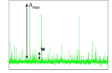
Figure 4.5: Snapshot for the SW-synchronized ($p$$=$$0.10$) landscape in a power-law noise environment ($\gamma$$=$$3$) for $N$$=$$10^{4}$ nodes.

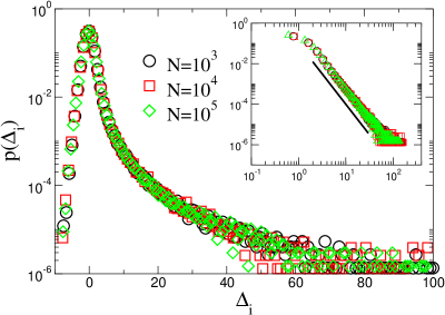
Figure 4.6: Disorder-averaged probability distributions in a power-law noise environment ($\gamma$$=$$3$) with $N$$=$$10^{4}$ nodes for the local height fluctuations for three system sizes indicated in the figure. Note the log-normal scales. The inset shows the same (for the positive domain) on log-log scales. The solid line corresponds to the slope of $\mu+1\approx 3$.

Here we show and discuss results for the power-law noise generated growth on SW networks. We have chosen two values of $\gamma$ governing the tail of the probability density for the noise: $\gamma$$=$$3$ and $\gamma$$=$$5$. For both of these cases the noise have a finite mean and variance. One can expect a power-law tail (at least for above the mean) for the probability density of the individual local height fluctuations $p(\Delta_{i})\sim 1/\Delta_{i}^{\mu+1}$, once the noise is “filtered through” the collective dynamics. In Fig. 4.5 we show a snapshot for the resulting synchronization landscape, indicating the presence of some rare but very large fluctuations above the mean. Since the local update rules lead to nonlinear (KPZ-like) effective interactions, we could not predict the exponent of the local height distribution. Instead, we constructed histograms representing $p(\Delta_{i})$. For the above two values of the noise exponent, $\gamma$$=$$3$ and $\gamma$$=$$5$, we observed power-law tail exponents for $p(\Delta_{i})\sim 1/\Delta_{i}^{\mu+1}$ as well, but with exponents clearly differing from that of the noise, $\mu$$\approx$$2$ and $\mu$$\approx$$4$, respectively. Figure 4.6 shows $p(\Delta_{i})$ for the former. The figure indicates that for large $\Delta_{i}$ a power-law tail develops, while fluctuations below the mean exhibit an exponential-like tail. This asymmetry is due to the asymmetry in the microscopic update rules: local minima were incremented by power-law distributed random amount, hence anomalously large deviations above the mean can emerge.

Then we analyzed the scaling behavior of the average and the extreme height fluctuations in the associated synchronization landscape. In the limit of large $N$, $w$ becomes system-size independent, while the extreme-height fluctuations above the mean diverge in a power-law fashion according to Eq. (4.10) [Fig. 4.7]. Fitting a power law for $N$$\geq$$10^{3}$ yields $\langle\Delta_{\max}\rangle\sim N^{0.47}$ and $\langle\Delta_{\max}\rangle\sim N^{0.25}$ for the two cases analyzed in Fig. 4.7, for $\gamma$$=$$3$ and $\gamma$$=$$5$, respectively.

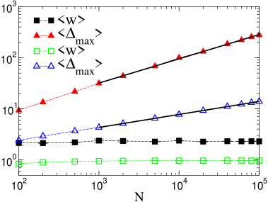
Figure 4.7: Steady-state scaling behavior of the average ($w$) and the extreme ($\Delta_{\max}$) fluctuations in the synchronization landscape for power-law noise with exponent $\gamma$$=$$3$ (filled symbols) and $\gamma$$=$$5$ (open symbols) using SW links with $p$$=$$0.10$. The straight solid-line segments are the best-fit power laws ($\langle\Delta_{\max}\rangle\sim N^{1/\mu}$ with $1/\mu$$=$$0.47$ and $1/\mu=0.25$, respectively) for the extreme fluctuations for system sizes $N\geq 10^{3}$, according to Eq. (4.10).

In order to understand the underlying reason for this divergence, we analyzed the histograms constructed for the probability density of the extreme height fluctuations $p(\Delta_{\max})$ [Fig. 4.8]. The shapes of these histograms suggest that the limit distribution is of Fréchet type. We constructed the histograms for the scaled variable $y=\Delta_{\max}/\langle\Delta_{\max}\rangle$. Then using $\mu=1/0.47=2.1$ and $\mu=1/0.25=4$ as implied by the scaling behavior of $\langle\Delta_{\max}\rangle$ [Eq. (4.10)], we plotted the similarly scaled Fréchet density Eq. (4.11) [Fig. 4.8(b)]. These results indicate that the effect of the random links in SW networks is again to decouple the local field variables, an in turn, the statistics of the extremes are governed by the Fréchet distribution. Consequently, the average size of the extremes diverges in a power-law fashion $\langle\Delta_{\max}\rangle\sim N^{1/\mu}$. This power-law divergence is not the result of a divergent length scale emerging from the cooperative effects of the interacting nodes. On the contrary, the local field variables become effectively independent using SW synchronization. The tail behavior for them (power-law with a possibly different exponent), however, is inherited from the noise. Hence, the statistics of the extremes will be of the Fréchet type, yielding a power-law increase of the average size of the largest fluctuations above the mean.

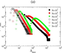
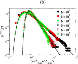
Figure 4.8: (a) Disorder-averaged probability distributions for the extreme height fluctuations for the SW-synchronized ($p$$=$$0.10$) landscape in a power-law noise environment for $\gamma$$=$$3$ (filled symbols) and $\gamma$$=$$5$ (open symbols) for three system sizes indicated in the figure. Note the log-log scales. (b) Scaled form of probability densities in Fig. 4.8. The solid curves correspond to the similarly scaled Fréchet density Eq. (4.11) for comparison.

The above picture is reasonably consistent in that the exponents for the tail behavior ($\sim$$1/\Delta_{i}^{\mu+1}$) for both the probability density of the local heights $p(\Delta_{i})$ and the extremes $p(\Delta_{\max})$ were within about $6\%$. Further, the average size of the extremes increases as $N^{1/\mu}$, in accordance with the underlying Fréchet distribution.

It is interesting to note that for $\mu$$\approx$$2$, formally, $p(\Delta_{i})$ does not have a finite variance (associated with the width $w=\sqrt{\langle(\tau_{i}-\bar{\tau})^{2}\rangle}=\sqrt{\langle(\Delta_{i})^{2}\rangle}$). Indeed, in the simulations we observed large fluctuations in $w$ and error bars of the order of the width itself. The “theoretical” divergence for $\mu$$=$$2$ is, of course, limited by the logarithm of a large but finite cutoff in the simulations. This anomalous (formally divergent) width is not related to a system-size dependent widening of the individual distributions controlled by a divergent correlation length. Rather, the individual distributions develop a heavy-tailed shape independent of the system size.

Examining the largest fluctuations below the mean reveals that they increase only logarithmically with the system size. This is simply the result of the exponential or similar tail of the individual local height fluctuations below the mean [Fig. 4.5], where the governing limit distribution is of the Gumbel type (Sec. 4.1.1).

The above results show, that SW synchronization can be efficient to control the average size of the fluctuations, but the largest fluctuations still diverge in a power-law fashion with the number of nodes. While the SW-network effectively decouples the fluctuations in the synchronization landscape, it cannot suppress power-law tails already present in local noise distribution. In fact, the inherited power-law tails for the local height fluctuations are even “heavier” than that of the corresponding noise, $\mu$$\approx$$2$ for $\gamma$$=$$3$ and $\mu$$\approx$$4$ for $\gamma$$=$$5$.

Chapter 5 SUMMARY AND FUTURE WORK

5.1 Summary

We studied synchronization phenomena in networks in general, and considered the scalability problem of the basic conservative synchronization schemes to test our results. Based on a mapping [39] between the evolution of the virtual time horizon for the basic conservative PDES scheme [55, 56] and kinetically grown non-equilibrium surfaces [73], we constructed a coarse-grained description for the scalability and performance of such large-scale parallel simulation schemes. These schemes can be applied to large spatially extended systems with short-range interactions and asynchronous dynamics. The one-site-per PE basic PDES was shown to exhibit KPZ-like kinetic roughening. This scheme is scalable in that the average progress rate of the PEs approaches a non-zero value. The spread of the virtual time horizon, however, diverges as the square root of the number of PEs, leading to “de-synchronization” and difficulties in data management.

In this work we considered the simplest (and in some regards, the worst case) scenario, where each nodes carries one site of the underlying physical system, hence synchronization with nearest neighbor PEs is required at every step. In actual parallel implementations the efficiency can be greatly increased by hosting many sites by each PE [47, 50, 51]. That way, communication between PEs is only required when local variables are to be updated on the boundary region of the sites hosted by the PEs (within the finite range of the interactions). While the above procedure clearly increases the utilization and reduces the actual communication overhead, it gives rise to an even faster growing early time regime in the simulated time horizon [139]. Since the PEs rarely need to synchronize, up to some crossover time, the evolution of the time horizon is governed by random deposition [73], a faster roughening growth, before eventually crossing over to the KPZ growth and a subsequent saturation.

Our goal here was to achieve synchronization without any global intervention. We constructed a specific version of the SW network, where each PE was connected to exactly one other randomly chosen PE. The extra synchronizational steps through the random links are merely used to control the width. The virtual time horizon for the SW-synchronized PDES scheme becomes “macroscopically” smooth and essentially exhibits mean-field like characteristics. The random links, on top of a regular lattice, generate an effective “mass” for the propagator of the virtual time horizon, corresponding to a nonzero correlation length. The width becomes finite, for an arbitrary small rate of synchronization through the random links, while the utilization remains nonzero, yielding a fully scalable PDES scheme. The former statement is only marginally weakened by observing that the extreme fluctuations in the time horizon can exhibit logarithmically large values as a function of the total number of PEs. The above predictions of the coarse-grained PDES model were confirmed by actually “simulating the simulations”. The generalization when random links are added to a higher-dimensional underlying regular lattice is clear: since the synchronization landscape of the 1D SW network is already macroscopically smooth, in higher dimensions it will be even more so [27] (i.e., the critical dimension of the underlying regular substrate is less than one).

We also studied the scalability properties for a causally constrained PDES scheme hosted by a network of computers where the network is scale-free following a “preferential attachment” construction [5, 102]. Here the PEs have to satisfy the general criterion that their simulated time should be smaller than that of all of their links’ simulated times in order to advance their local time. Despite some nodes in the network having abnormally large connectivity (as a result of the scale-free nature of the degree distribution), we found that the computational phase of the algorithm is only marginally non-scalable. The utilization exhibited slow logarithmic decay as a function of the number of PEs. At the same time, the width of the time horizon diverged logarithmically slowly, rendering the measurement phase of the simulations marginally non-scalable as well. The implication of this finding is that the internet, which is already exploited for distributed computing for mostly “embarrassingly parallel” problems through existing GRID-based schemes [17, 16], may have the potential to accommodate efficient complex system simulations (such as asynchronous PDES) where the nodes frequently have to synchronize with each other. An intriguing question to pursue is how the logarithmic divergence of the surface fluctuations observed here can be related to the collective behavior (in particular, the finite-size effects of the magnetic susceptibility) of Ising ferromagnets on scale-free networks [140, 141, 142, 143] with the same degree distribution.

We also considered the extreme-height fluctuations in this prototypical model with local relaxation, unbounded local variables, and in the presence of exponential or power-law tailed noise. We showed that when the interaction topology is extended to include random links in a SW fashion, the local height variables become effectively independent and the statistics of the extremes is governed by the FTG or the Fréchet distribution, respectively. For both types of noise, the average width of the synchronization landscape becomes independent of the system size. The extreme fluctuations increase only logarithmically with the number of nodes for exponential-like noise and in a power-law fashion for the power-law noise. These findings directly addresses synchronizability in generic SW-coupled systems where relaxation through the links is the relevant node-to-node process and effectively governs the dynamics. We illustrated our results on an actual synchronizational problem in the context of scalable parallel simulations.

Our findings are also closely related to critical phenomena and collective phenomena on networks [2, 3, 36, 144]. In particular, in recent years, a number of prototypical models have been investigated on SW networks [19, 21, 22, 23, 25, 26, 27, 28, 29, 30, 31, 32, 33, 34, 38, 105, 145, 146, 147, 148, 149, 150, 151]. Of these, the ones most closely related to our work are the XY model [25], the EW model [27, 28, 29], and diffusion [27, 28, 29, 30, 31, 32, 33, 34] on SW networks. The findings suggest that systems without inherent frustration exhibit (strict or anomalous) [27, 28, 29, 34, 151] mean-field-like behavior when the original short-range interaction topology is modified to a SW network. In essence, the SW couplings, although sparse, induce an effective relaxation to the mean of the respective local field variables, and in turn, the system exhibits a mean-field-like behavior [151]. This effect is qualitatively similar to those observed in models with “annealed” long-range random couplings [32, 152, 153], but on (quenched) SW networks, the scaling properties can differ from those with annealed interactions [27, 28, 29, 34, 151].

5.2 Future Work

In many real networks the cost of the random and arbitrarily long-range links could be unaffordable. Recent works show that in cortical [154] and on-chip logic networks [155] power-law-suppressed link-length distributions are observed because these are spatially embedded networks with wiring-costs [156]. To study these networks one can consider a special model of SW network with distance-dependent power-law probability distribution of long-range links, where the probability of two nodes being connected is $r^{-\alpha}$, with a varying exponent $\alpha$ and the distance $r$ between the nodes [28, 29]. By varying the exponent $\alpha$, one can control the distribution of the random links. Changing $\alpha$ changes the topology of the network from the “plain” SW in which there is no wiring cost as we discussed in Chapter 3 ($\alpha$$=$$0$), to a short-range network in which only nearest neighbor links are present ($\alpha$$=$$\infty$).

The synchronization problem described in the previous chapters can also be studied on this network. The roughness of the time-surface as a function of the exponent $\alpha$ can give valuable information about the conditions on the scalability of the PDES. One can follow the same way of constructing the network; one random link per PE (chosen with distance-dependent probability) in addition to the nearest neighbors. The width of the linear EW model obtained through adjacency matrix diagonalization exhibits a smooth transition from system-size independent width (plain SW) to the KPZ width dependence ($\langle w^{2}\rangle$$\sim$$N$) [Fig. 5.1(a)].

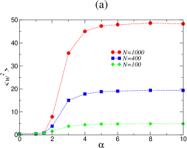
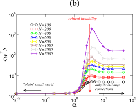
Figure 5.1: (a) Width as a function of $\alpha$ for the EW model on a $1/r^{\alpha}$ SW network. (b) Width as a function of $\alpha$ for the conservative synchronization dynamics on a $1/r^{\alpha}$ SW network.

Simulating the “microscopic” dynamics in the actual PDES (incrementing the “local” minima) can give rise to nonlinear effects, typical for the KPZ surface, as can be seen in Fig. 5.1(b). We see the transition from plain SW to KPZ again but through critical instability. By analyzing the Fig. 5.1(b) we can argue that for some critical range of $\alpha$, the scalability of the PDES is worse than the BCS scheme (short-range network). Another surface growth model, single-step model (KPZ class), has also the same effect suggesting that as long as there is nonlinearity in the growth, the similar peaks in the width will be seen.

Another possible future work might be to study the scale-free Barabási-Albert network further. In the preferential attachment process to construct the BA network at each time step we added only one node to the network ($m$$=$$1$). This led to logarithmic (marginal) scalability of the PDES scheme. It might help to increase $m$ in suppressing the virtual time fluctuations and thus making the PDES scheme fully scalable in this network as well.

LITERATURE CITED

Appendix A Steady-State Structure Factor in Linear Growth Models

The time evolution of linearly interacting local field variables on a network can be written in the form of a Langevin equation as

$$\partial_{t}\tau_{i}(t)=-\sum_{j}\Gamma_{ij}\tau_{j}(t)+\eta_{i}(t)\;,$$ (A.1)

where $\Gamma_{ij}$ is the coupling matrix containing the topology of the network, and $\eta_{i}(t)$ is the noise delta-correlated in space/time with zero average as expressed in the following equations

$$\langle\eta_{i}(t)\rangle=0$$ (A.2)

and

$$\langle\eta_{i}(t)\eta_{j}(t^{\prime})\rangle=2D\delta_{i,j}\delta(t-t^{\prime})\;.$$ (A.3)

For the nearest-neighbor network $\Gamma_{ij}$ is the discrete Laplacian

$$\Gamma_{ij}=\Gamma_{ij}^{0}=2\delta_{i,j}-\delta_{i-1,j}-\delta_{i+1,j}\;.$$ (A.4)

For the maximal-distance network

$$\Gamma_{ij}=\Gamma_{ij}^{0}+\gamma(\delta_{i,j}-\delta_{i-N/2,j})\;.$$ (A.5)

For the fully-connected network

$$\Gamma_{ij}=\Gamma_{ij}^{0}+\gamma(\delta_{i,j}-\frac{1}{N})\;.$$ (A.6)

We consider cases where $\Gamma_{ij}$ is translationally invariant, i.e., it does not depend on $i$ and $j$ explicitly but depends only on the distance $l$$=$$i-j$ between them,

$$\Gamma_{ij}=\Gamma(i-j)=\Gamma(l)\;.$$ (A.7)

The structure factor [as defined through Eq. (2.9)] contains all the physics we need to describe the evolution of the network. One needs the Fourier transforms of the local field variables defined as

$$\tilde{\tau}_{k}(t)=\sum_{j=1}^{N}e^{-ikj}[\tau_{j}(t)-\bar{\tau}(t)]\;.$$ (A.8)

Taking the Fourier transformation of Eq. (A.1) one finds

$$\partial_{t}\tilde{\tau}_{k}(t)=-\tilde{\Gamma}(k)\tilde{\tau}_{k}(t)+\tilde{\eta}_{k}(t)\;,$$ (A.9)

where $\tilde{\Gamma}(k)$ and $\tilde{\eta}_{k}(t)$ are the Fourier transforms of $\Gamma(l)$ and $\eta_{i}(t)$, respectively. The wave number $k$ goes from $1$ to $N$$-$$1$ since we exclude the zero-mode contribution, $\tilde{\tau}_{0}(t)$$\equiv$$0$ for all $t$. We can see that the evolution decouples for different $k$ values in Fourier space. The second moment of the Fourier transform of the noise is

$$\langle\eta_{k}(t)\eta_{k^{\prime}}(t^{\prime})\rangle=2DN\delta_{k+k^{\prime},0}\delta(t-t^{\prime})\;.$$ (A.10)

Integrating Eq. (A.9) we obtain

$$\tilde{\tau}_{k}(t)=e^{-\tilde{\Gamma}(k)t}\int_{0}^{t}dt^{\prime}e^{\tilde{\Gamma}(k)t^{\prime}}\tilde{\eta}_{k}(t^{\prime})\;.$$ (A.11)

By using Eq. (A.11) one can write the equal-time correlations for the local field variables as

$$\langle\tilde{\tau}_{k}(t)\tilde{\tau}_{k^{\prime}}(t)\rangle=e^{-[\tilde{\Gamma}(k)+\tilde{\Gamma}(k^{\prime})]t}\int dt^{\prime}\int dt^{\prime\prime}e^{\tilde{\Gamma}(k)t^{\prime}+\tilde{\Gamma}(k^{\prime})t^{\prime\prime}}\langle\tilde{\eta}_{k}(t^{\prime})\tilde{\eta}_{k^{\prime}}(t^{\prime\prime})\rangle\;.$$ (A.12)

By substituting the second moment of the Fourier transform of the noise [Eq. (A.10)] into Eq. (A.12), and by using the basic property of the delta function $\delta(t^{\prime}-t^{\prime\prime})$ in the integral, one obtains

$$\langle\tilde{\tau}_{k}(t)\tilde{\tau}_{k^{\prime}}(t)\rangle=2DN\delta_{k+k^{\prime},0}e^{-[\tilde{\Gamma}(k)+\tilde{\Gamma}(k^{\prime})]t}\int_{0}^{t}dt^{\prime}e^{[\tilde{\Gamma}(k)+\tilde{\Gamma}(k^{\prime})]t^{\prime}}\;.$$ (A.13)

The integral in the equation above can be evaluated easily and one obtains

$$\langle\tilde{\tau}_{k}(t)\tilde{\tau}_{k^{\prime}}(t)\rangle=2DN\delta_{k+k^{\prime},0}e^{-[\tilde{\Gamma}(k)+\tilde{\Gamma}(k^{\prime})]t}\frac{e^{[\tilde{\Gamma}(k)+\tilde{\Gamma}(k^{\prime})]t}-1}{\tilde{\Gamma}(k)+\tilde{\Gamma}(k^{\prime})}\;.$$ (A.14)

After rearranging the terms and rewriting the delta function as $\delta_{k+k^{\prime},0}$$=$$\delta_{k^{\prime},-k}$, one obtains

$$\langle\tilde{\tau}_{k}(t)\tilde{\tau}_{k^{\prime}}(t)\rangle=\frac{2DN\delta_{k^{\prime},-k}}{\tilde{\Gamma}(k)+\tilde{\Gamma}(-k)}\{1-e^{-[\tilde{\Gamma}(k)+\tilde{\Gamma}(-k)]t}\}\;.$$ (A.15)

From the present form of Eq. (A.15) and by using Eq. (2.9) one can deduce the general time-dependent structure factor as

$$S(k,t)=\frac{2D}{\tilde{\Gamma}(k)+\tilde{\Gamma}(-k)}\{1-e^{-[\tilde{\Gamma}(k)+\tilde{\Gamma}(-k)]t}\}\;.$$ (A.16)

In the steady-state ($t$$\to$$\infty$) the structure factor becomes

$$S(k)=\lim_{t\to\infty}S(k,t)=\frac{2D}{\tilde{\Gamma}(k)+\tilde{\Gamma}(-k)}\;.$$ (A.17)

The steady-state structure factor can be calculated easily once the Fourier transform of the coupling function $\tilde{\Gamma}(k)$ is known. Now we calculate the structure factors for a few simple interaction topologies.

A.1 Nearest-neighbor network

The coupling matrix $\Gamma_{ij}$ for the nearest-neighbor network is a Laplacian,

$$\Gamma_{ij}=\Gamma_{ij}^{0}=2\delta_{i,j}-\delta_{i-1,j}-\delta_{i+1,j}\;,$$ (A.18)

and one can rewrite the equation above by using the distance-dependent coupling function

$$\Gamma^{0}(l)=2\delta_{l,0}-\delta_{l,1}-\delta_{l,-1}\;,$$ (A.19)

then the Fourier transform of $\Gamma^{0}(l)$ becomes

$$\tilde{\Gamma}^{0}(k)=(2-e^{ik}-e^{-ik})=2[1-\cos(k)]\;.$$ (A.20)

So the structure factor is, as in Eq. (2.10),

$$S(k)=\frac{D}{2[1-\cos(k)]}\;.$$ (A.21)

A.2 Maximal-distance network

Starting with the coupling matrix for the maximal-distance network, one obtains the distance-dependent coupling function as

$$\Gamma(l)=\Gamma^{0}(l)+\gamma(\delta_{l,0}-\delta_{l,\frac{N}{2}})\;.$$ (A.22)

Then the Fourier transform $\tilde{\Gamma}(k)$ becomes,

$$\tilde{\Gamma}(k)=\tilde{\Gamma}^{0}(k)+\gamma(1-e^{\frac{ikN}{2}})=2[1-\cos(k)]+\gamma(1-e^{\frac{ikN}{2}}).\;.$$ (A.23)

By using Eq. (A.17) we obtain

$$S(k)=\frac{D}{2[1-\cos(k)]+\gamma[1-\cos(\frac{kN}{2})]}\;.$$ (A.24)

A.3 Fully-connected network

Hasan Guclu

In this network, as we mentioned in Chapter 3, each node is connected to all other nodes with strength $\gamma/N$ and the coupling function is

$$\Gamma(l)=\Gamma^{0}(l)+\gamma(\delta_{l,0}-\frac{1}{N})\;.$$ (A.25)

Its Fourier transform becomes

$$\tilde{\Gamma}(k)=\tilde{\Gamma}^{0}(k)+\gamma=2[1-\cos(k)]+\gamma\;.$$ (A.26)

Thus one can obtain the structure factor as

$$S(k)=\frac{D}{2[1-\cos(k)]+\gamma}\;.$$ (A.27)

LITERATURE CITED

- [1] Y. Bar-Yam, Dynamics of Complex Systems (Studies in Nonlinearity) (Westview Press, Boulder, CO, 1997). [http://necsi.org/publications/dcs/index.html]
- [2] R. Albert and A.-L. Barabási, “Statistical mechanics of complex networks”, Rev. Mod. Phys. 74, pp. 47–97 (2002). [cond-mat/0106096] 111Where available the references to the preprint server, arxiv.org are given. Papers may be downloaded from http://arxiv.org/abs/*, where * is the reference. For example; the link for the paper cond-mat/0311575 is http://arxiv.org/cond-mat/0311575. For preprints this is a primary reference; for published papers there may be differences between the published versions and the preprint.
- [3] S.N. Dorogovtsev and J.F.F. Mendes, “Evolution of networks”, Adv. Phys. 51, pp. 1079–1187 (2002). [cond-mat/0106144]
- [4] M.E.J. Newman, “The structure and function of complex networks”, SIAM Review 45, pp. 167–256 (2002). [cond-mat/0303516]
- [5] A.-L. Barabási and R. Albert, “Emergence of scaling in random networks”, Science 286, pp. 509–512 (1999). [cond-mat/9910332]
- [6] M. Faloutsos, P. Faloutsos, and C. Faloutsos, “On power-law relationships of the Internet topology”, Proc. ACM SIGCOMM, Comput. Commun. Rev. 29, pp. 251–262 (1999).
- [7] E.J. Lerner, “What’s wrong with the electric grid?”, The Industrial Physicist, Oct./Nov., pp. 8–13 (2003).
- [8] G. Korniss, M.A. Novotny, H. Guclu, Z. Toroczkai, and P.A. Rikvold, “Suppressing roughness of virtual times in parallel discrete-event simulations”, Science 299, pp. 677–679 (2003). [cond-mat/0302050]
- [9] Y. Rabani, A. Sinclair, and R. Wanka, “Local divergence of Markov chains and the analysis of iterative load-balancing schemes”, in Proceedings of the 39th Annual Symposium on Foundations of Computer Science, pp. 694–703 (IEEE Comput. Soc., Los Alamitos, CA, 1998).
- [10] L.L. Peterson and B.S. Davie, Computer Networks, A Systems Approach, 2nd edn (Morgan Kaufmann, San Francisco, CA, 2000).
- [11] R. Albert, H. Jeong, and A.-L. Barabási, “Internet: Diameter of the World-Wide Web”, Nature 401, pp. 130–131 (1999).
- [12] H. Jeong, B. Tombor, R. Albert, Z.N. Oltvai, and A.-L. Barabási, “The large-scale organization of metabolic networks”, Nature 407, pp. 651–654 (2000). [cond-mat/0010278]
- [13] S. Eubank, H. Guclu, V.S.A. Kumar, M.V. Marathe, A. Srinivasan, Z. Toroczkai, and N. Wang, “Modelling disease outbreaks in realistic urban social networks”, Nature 429, pp. 180–184 (2004).
- [14] R. Senturk, “Narrative social structure” (Stanford University Press, Stanford, CA, 2005).
- [15] See, e.g., www.top500.org and www.research.ibm.com/bluegene/.
- [16] S. Kirkpatrick, “Rough times ahead”, Science 299, pp. 668–669 (2003).
- [17] See, e.g., www.gridforum.org and setiathome.ssl.berkeley.edu.
- [18] S. Milgram, “The small-world problem”, Psychology Today 1, pp. 61–68 (1967).
- [19] D.J. Watts and S.H. Strogatz, “Collective dynamics of small-world networks”, Nature 393, pp. 440–442 (1998).
- [20] P. Erdős and A. Rényi, “On the evolution of random graphs”, Publ. Math. Inst. Hung. Acad. Sci. 5, pp. 17–61 (1960).
- [21] R.T. Scalettar, “Critical properties of an Ising model with dilute long range interactions”, Physica A 170, pp. 282–290 (1991).
- [22] M. Gitterman, “Small-world phenomena in physics: the Ising model”, J. Phys. A 33, pp. 8373–8381 (2000).
- [23] A. Barrat and M. Weigt, “On the properties of small-world network models”, Eur. Phys. J. B 13, pp. 547–560 (2000). [cond-mat/9903411]
- [24] M.A. Novotny and S.M. Wheeler, “On the possibility of quasi small-world nanomaterials”, Braz. J. Phys. 34, pp. 395–400 (2004). [cond-mat/0308602]
- [25] B.J. Kim, H. Hong, P. Holme, G.S. Jeon, P. Minnhagen, and M.Y. Choi, “XY model in small-world networks”, Phys. Rev. E 64, 056135 [5 pages] (2001). [cond-mat/0108392]
- [26] H. Hong, M.Y. Choi, and B.J. Kim, “Phase ordering on small-world networks with nearest-neighbor edges”, Phys. Rev. E 65, 047104 [4 pages] (2002). [cond-mat/0203177]
- [27] B. Kozma, M.B. Hastings, and G. Korniss, “Roughness scaling for Edwards-Wilkinson relaxation in small-world networks”, Phys. Rev. Lett. 92, 108701 [4 pages] (2004). [cond-mat/0309196]
- [28] B. Kozma, M.B. Hastings, and G. Korniss, “Processes on annealed and quenched power-law small-world networks”, in Noise in Complex Systems and Stochastic Dynamics III, edited by L.B. Kish, K. Lindenberg, Z. Gingl, Proceedings of SPIE 5845, pp. 130–138 (SPIE, Bellingham, WA, 2005) .
- [29] B. Kozma, M.B. Hastings, and G. Korniss, “Diffusion Processes on Power-Law Small-World Networks”, Phys. Rev. Lett. (in press, 2005). [cond-mat/0501509]
- [30] R. Monasson, “Diffusion, localization and dispersion relations on small-world lattices”, Eur. Phys. J. B 12, pp. 555–567 (1999). [cond-mat/9903347]
- [31] S. Jespersen, I.M. Sokolov, and A. Blumen, “Relaxation properties of small-world networks”, Phys. Rev. E 62, pp. 4405–4408 (2002). [cond-mat/0004214]
- [32] S. Jespersen and A. Blumen, “Small-world networks: Links with long-tailed distributions”, Phys. Rev. E 62, pp. 6270–6274 (2002). [cond-mat/0009082]
- [33] E. Almaas, R.V. Kulkarni, and D. Stroud, “Characterizing the structure of small-world networks”, Phys. Rev. Lett. 88, 098101 [4 pages] (2002). [cond-mat/0109227]
- [34] M.B. Hastings, “An -expansion for small-world networks”, Eur. Phys. J. B 42, pp. 297–301 (2004). [cond-mat/0407374]
- [35] K. Wiesenfeld, P. Colet, and S.H. Strogatz, “Synchronization transitions in a disordered josephson series array”, Phys. Rev. Lett. 76, pp. 404–407 (1996).
- [36] S.H. Strogatz, “Exploring complex networks”, Nature 410, pp. 268–276 (2001).
- [37] M. Barahona and L.M. Pecora, “Synchronization in small-world systems, Phys. Rev. Lett. 89, 054101 [4 pages] (2002). [nlin.CD/0112023]
- [38] H. Hong, B.J. Kim, and M.Y. Choi, “Comment on ‘Ising model on a small-world network’ ”, Phys. Rev. E 66, 018101 [2 pages] (2002). [cond-mat/0204357]
- [39] G. Korniss, Z. Toroczkai, M.A. Novotny, and P.A. Rikvold, “From massively parallel algorithms and fluctuating time horizons to non-equilibrium surface growth” Phys. Rev. Lett. 84, pp. 1351–1354 (2000). [cond-mat/9909114]
- [40] R. Fujimoto, “Parallel discrete event simulation”, Commun. of the ACM 33, pp. 30–53 (1990).
- [41] D.M. Nicol and R.M. Fujimoto, “Parallel simulation today”, Ann. Oper. Res. 53, pp. 249–285 (1994).
- [42] B.D. Lubachevsky, “Fast simulation of multicomponent dynamic systems”, Bell Labs Tech. J. 5 (April-June), pp. 134–156 (2000). [cs.DS/0405077]
- [43] A. Kolakowska, M. A. Novotny, in Progress in Computer Science Research (Nova Science Publishers, in press) (2004). [cs.DC/0409032]
- [44] K. Hwang, Advanced Computer Architecture: Parallelism, Scalability, and Programmability (McGraw–Hill, New York, NY, 1993).
- [45] K. Binder and D.W. Heermann, Monte Carlo Simulation in Statistical Physics : An Introduction (Springer, Berlin, 1998).
- [46] A.G. Greenberg, B.D. Lubachevsky, D.M. Nicol, and P.E. Wright, “Efficient Massively parallel simulation of dynamic channel assignment schemes for wireless cellular communications”, Proc. 8th Workshop on Parallel and Distributed Simulation (PADS’94), pp. 187–194 (SCS, San Diego, CA, 1994).
- [47] G. Korniss, M.A. Novotny, and P.A. Rikvold, “Parallelization of a dynamic Monte Carlo algorithm: A partially rejection-free conservative approach”, J. Comput. Phys. 153, pp. 488–508 (1999). [cond-mat/9812344]
- [48] G. Korniss, C.J. White, P.A. Rikvold, and M.A. Novotny, “Dynamic phase transition, universality, and finite-size scaling in the two-dimensional kinetic Ising model in an oscillating field”, Phys. Rev. E 63, 016120 [15 pages] (2001). [cond-mat/0008155]
- [49] E. Deelman, B.K. Szymanski, and T. Caraco, “Simulating lyme disease using parallel discrete-event simulations”, in Proc. 28th Winter Simulation Conference, pp. 1191–1198 (ACM, New York, NY, 1996).
- [50] Y. Shim and J.G. Amar, “Rigorous synchronous relaxation algorithm for parallel kinetic Monte Carlo simulations of thin film growth”, Phys. Rev. B 71, 115436 [12 pages] (2005). [cond-mat/0406540]
- [51] Y. Shim and J.G. Amar, “Semirigorous synchronous sublattice algorithm for parallel kinetic Monte Carlo simulations of thin film growth”, Phys. Rev. B 71, 125432 [13 pages] (2005). [cond-mat/0406379]
- [52] D.M. Nicol, “Performance issues for distributed battlefield simulations”, Proc. Conf. Winter. Simul. ed. by A. Thesen, H. Grant, and W.D. Kelton, pp. 624–628 (1987).
- [53] J. Cowie, D.M. Nicol, and A. Ogielski, “Modeling the global Internet”, IEEE Computing in Science and Engineering 1, pp. 42–50 (1999).
- [54] R.J. Glauber, “Time-dependent statistics of the Ising model”, J. Math. Phys. 4, pp. 294–307 (1963).
- [55] B.D. Lubachevsky, “Efficient parallel simulations of asynchronous cellular arrays”, Complex Systems 1, pp. 1099–1123 (1987). [cs.DC/0502039]
- [56] B.D. Lubachevsky, “Efficient parallel simulations of dynamic Ising spin systems”, J. Comput. Phys. 75, pp. 103–122 (1988).
- [57] D.R. Jefferson, “Virtual time”, Assoc. Comput. Mach. Trans. Programming Languages and Systems 7, pp. 404–425 (1985).
- [58] K.M. Chandy and J. Misra, “Distributed simulation: A case study in design and verification of distributed programs”, IEEE Trans. Softw. Eng. SE-5, pp. 440–452 (1979).
- [59] K.M. Chandy, and J. Misra, “Asynchronous distributed simulation via a sequence of parallel computations”, Commun. ACM 24, pp. 198–205 (1981).
- [60] E. Deelman and B.K. Szymanski, “Breadth-first rollback in spatially explicit simulations”, Proc. of the 11th Workshop on Parallel and Distributed Simulation, PADS ’97, pp. 124–131 (IEEE Computer Society, Los Alamitos, CA, 1997).
- [61] C.D. Carothers, K.S. Perumalla, and R.M. Fujimoto, “Efficient optimistic parallel simulations using reverse computation”, ACM Transactions on Modeling and Computer Simulation (TOMACS) 9, pp. 224–253 (1999).
- [62] G. Chen and B.K. Szymanski, “Lookback: a new way of exploiting parallelism in discrete event simulation”, Proc. of the 16th Workshop on Parallel and Distributed Simulation, PADS ’02, pp. 153–162 (IEEE Computer Society, Washington, DC, 2002).
- [63] L. N. Shchur and M. A. Novotny, “Evolution of time horizons in parallel and grid simulations”, Phys. Rev. E 70, 026703 [9 pages] (2004). [cond-mat/0401229]
- [64] A.G. Greenberg, S. Shenker, and A.L. Stolyar, “Asynchronous updates in large parallel systems”, Performance Eval. Rev. 24, pp. 91–103 (1996).
- [65] P.M.A. Sloot, B.J. Overeinder, and A. Schoneveld, “Self-organized criticality in simulated correlated systems”, Comput. Phys. Commun. 142, pp. 76–81 (2001).
- [66] A. Schoneveld, “Parallel complex systems simulation”, Ph.D. Thesis, Universiteit van Amsterdam (1999).
- [67] P. Bak, C. Tang, and K. Wiesenfeld, “Self-organized criticality: An explanation of noise”, Phys. Rev. Lett. 59, pp. 381–384 (1987).
- [68] P. Bak, C. Tang, and K. Wiesenfeld, “Self-organized criticality”, Phys. Rev. A 38, pp. 364–374 (1988).
- [69] Frontiers in Problem Solving: Phase Transitions and Complexity, ed. by T. Hogg, B.A. Huberman, and C. Williams, Artif. Intell. 81, issue 1-2 (1996).
- [70] R. Monasson, R. Zecchina, S. Kirkpatrick, B. Selman, and L. Troyansky, “Determining computational complexity from characteristic phase transitions” Nature 400, pp. 133–137 (1999).
- [71] D.M. Nicol, “Performance bounds on parallel self-initiating discrete-event simulations”, ACM Trans. Model. Comput. Simul. 1, pp. 24–50 (1991).
- [72] R.E. Felderman and L. Kleinrock, “Bounds and approximations for self-initiating distributed simulation without lookahead”, ACM Trans. Model. Comput. Simul. 1, 386 (1991).
- [73] A.-L. Barabási and H.E. Stanley, Fractal Concepts in Surface Growth, (Cambridge Univ. Press, Cambridge, MA, 1995).
- [74] T. Halpin-Healy and Y.-C. Zhang, “Kinetic roughening phenomena, stochastic growth, directed polymers, and all that”, Physics Reports 254, pp. 215–414 (1995).
- [75] J. Krug, “Origins of scale invariance in growth processes”, Adv. Phys. 46, pp. 139–282 (1997).
- [76] F. Family and T. Vicsek, “Scaling of the active zone in the Eden process on percolation networks and the ballistic deposition model”, J. Phys. A 18, pp. L75–L81 (1985).
- [77] Z. Toroczkai, G. Korniss, S. Das Sarma, and R.K.P. Zia, “Extremal point densities of interface fluctuations”, Phys. Rev. E 62, pp. 276–294 (2000). [cond-mat/0002143]
- [78] J. Krug and P. Meakin, “Universal finite-size effects in the rate of growth process”, J. Phys. A 23, pp. L987–L994 (1990).
- [79] G. Korniss, M.A. Novotny, A.K. Kolakowska, and H. Guclu, “Statistical properties of the simulated time horizon in conservative parallel discrete-event simulations”, SAC 2002, Proceedings of the 2002 ACM Symposium on Applied Computing, pp. 132–138 (2002).
- [80] A. Kolakowska, M.A. Novotny, and G. Korniss, “Algorithmic scalability in globally constrained conservative parallel discrete-event simulations of asynchronous systems”, Phys. Rev. E 67, 046703 [13 pages] (2003). [cs.DC/0211013]
- [81] A. Kolakowska, M.A. Novotny, and P.A. Rikvold, “Update statistics in conservative parallel discrete event simulations of asynchronous systems”, Phys. Rev. E 68, 046705 [14 pages] (2003). [cond-mat/0306222]
- [82] A. Kolakowska and M.A. Novotny, “Discrete-event analytic technique for surface growth problems”, Phys. Rev. B 69, 075407 [5 pages] (2004). [cond-mat/0311015]
- [83] M. Plischke, Z. Rácz, and D. Liu, “Time-reversal invariance and universality of two-dimensional growth models”, Phys. Rev. B 35, pp. 3485–3495 (1987).
- [84] M. Kardar, G. Parisi, and Y.-C. Zhang, “Scaling of growing interfaces”, Phys. Rev. Lett. 56, pp. 889–892 (1986).
- [85] M. Burgers, The Nonlinear Diffusion Equation (Riedel, Boston, MA, 1974).
- [86] S.F. Edwards and D.R. Wilkinson, “The surface statistics of a granular aggregate”, Proc. R. Soc. London, Ser. A 381, pp. 17–31 (1982).
- [87] Z. Toroczkai, G. Korniss, M. A. Novotny, and H. Guclu, “Virtual time horizon control via communication network design”, in Computational Complexity and Statistical Physics, edited by A. Percus, G. Istrate, and C. Moore, Santa Fe Institute Studies in the Sciences of Complexity Series (Oxford University Press, 2004). [cond-mat/0304617]
- [88] G. Foltin, K. Oerding, Z. Rácz, R.L. Workman, and R.K.P. Zia, “Width distribution for random-walk interfaces”, Phys. Rev. E 50, pp. R639–R642 (1994).
- [89] M. Plischke, Z. Rácz, and R.K.P. Zia, “Width distribution of curvature-driven interfaces: A study of universality”, Phys. Rev. E 50, pp. 3589–3593 (1994).
- [90] Z. Rácz and M. Plischke, “Width distribution for -dimensional growth and deposition processes”, Phys. Rev. E 50, pp. 3530–3537 (1994).
- [91] T. Antal and Z. Rácz, “Dynamic scaling of width distribution in Edwards–Wilkinson type models of interface dynamics”, Phys. Rev. E 54, pp. 2256–2260 (1996). [cond-mat/9510170]
- [92] G. Korniss, M.A. Novotny, Z. Toroczkai, and P.A. Rikvold, “Nonequilibrium surface growth and scalability of parallel algorithms for large asynchronous systems”, Computer Simulation Studies in Condensed Matter Physics XIII, Springer Proceedings in Physics, Vol. 86, editors D.P. Landau, S.P. Lewis, and H.-B. Schüttler (Springer-Verlag, Berlin, Heidelberg), pp. 183–188 (2001). [cond-mat/0002469]
- [93] E. Marinari, A. Pagnani, and G. Parisi, “Critical exponents of the KPZ equation via multi-surface coding numerical simulations”, J. Phys. A: Math. Gen. 33, pp. 8181–8192 (2000). [cond-mat/0005105]
- [94] J.M. Kim and J.M. Kosterlitz, “Growth in a restricted solid-on-solid model”, Phys. Rev. Lett. 62, pp. 2289–2292 (1989).
- [95] E. Marinari, A. Pagnani, G. Parisi, and Z. Rácz, “Width distributions and the upper critical dimension of KPZ interfaces” Phys. Rev. E 65, 026136 [4 pages] (2002). [cond-mat/0105158]
- [96] B. Bollobás, Random Graphs (Cambridge University Press, Cambridge, UK, 2001).
- [97] W. Feller, An Introduction to Probability Theory and Its Applications, Vol. 1, 3rd ed. (Wiley, New York, NY, 1968).
- [98] W. Feller, An Introduction to Probability Theory and Its Applications, Vol. 2, 3rd ed. (Wiley, New York, NY, 1971).
- [99] H. Guclu, G. Korniss, Z. Toroczkai, and M.A. Novotny, “Small-world synchronized computing networks for scalable parallel discrete-event simulations”, in Complex Networks, edited by E. Ben-Naim, H. Frauenfelder, and Z. Toroczkai, Lecture Notes in Physics 650, pp. 255–275 (Springer-Verlag, Berlin, 2004).
- [100] http://www.netcraft.com/survey/
- [101] http://www.c-i-a.com
- [102] A.-L. Barabási, R. Albert, and H. Jeong, “Mean-field theory for scale-free random networks”, Physica A 272, pp. 173–187 (1999). [cond-mat/9907068]
- [103] H. Guclu and G. Korniss, “Extreme fluctuations in small-world networks with relaxational dynamics”, Phys. Rev. E 69, 065104(R) [4 pages] (2004). [cond-mat/0311575]
- [104] H. Guclu and G. Korniss, “Extreme fluctuations in small-world-coupled autonomous systems with relaxational dynamics”, Fluctuations and Noise Letters 5, pp. L43-L62 (2005).
- [105] D.J. Watts, Small Worlds (Princeton Univ. Press, Princeton, NJ, 1999).
- [106] R.A. Fisher and L.H.C. Tippett, “The frequency distribution of the largest or smallest member of a sample”, Proc. Camb. Philos. Soc. 24, pp. 180–191 (1928).
- [107] E.J. Gumbel, Statistics of Extremes (Columbia University Press, New York, NY, 1958).
- [108] Extreme Value Theory and Applications, edited by J. Galambos, J. Lechner, and E. Simin (Kluwer, Dordrecht, 1994).
- [109] S.T. Bramwell, P.C.W. Holdsworth, and J.-F. Plinton, “Universality of rare fluctuations in turbulance and critical phenomena”, Nature 396, pp. 552–554 (1998).
- [110] S. Raychaudhuri, M. Cranston, C. Przybyla, and Y. Shapir, “Maximal height scaling of kinetically growing surfaces” Phys. Rev. Lett. 87, 136101 [4 pages] (2001). [cond-mat/0105176]
- [111] S.T. Bramwell, K. Christensen, J.-Y. Fortin, P.C.W. Holdsworth, H.J. Jensen, S. Lise, J.M. López, M. Nicodemi, J.-F. Pinton, and M. Sellitto, “Universal fluctuations in correlated system”, Phys. Rev. Lett. 84, pp. 3744–3747 (2000). [cond-mat/9912255]
- [112] N.W. Watkins, S.C. Chapman, and G. Rowlands, “Comment on ‘universal fluctuations in correlated systems’ ”, Phys. Rev. Lett. 89, 208901 [1 page] (2002). [cond-mat/0209398]
- [113] S.T. Bramwell, K. Christensen, J.-Y. Fortin, P.C.W. Holdsworth, H.J. Jensen, S. Lise, J.M. López, M. Nicodemi, J.-F. Pinton, and M. Sellitto, “Reply to ‘comment on ‘universal fluctuations in correlated systems’ ’ ”, Phys. Rev. Lett. 89, 208902 [1 page] (2002). [cond-mat/0209416]
- [114] S.T. Bramwell, J.-Y. Fortin, P.C.W. Holdsworth, S. Peysson, J.-F. Pinton, B. Portelli, and M. Sellitto, “Magnetic fluctuations in the classical XY model: The origin of an exponential tail in complex systems”, Phys. Rev. E 63, 041106 [22 pages] (2001). [cond-mat/0008093]
- [115] V. Aji and N. Goldenfeld, “Fluctuations in finite critical and turbulent systems”, Phys. Rev. Lett. 86, pp. 1007–1010 (2001). [cond-mat/0008243]
- [116] T. Antal, M. Droz, G. Györgyi, and Z. Rácz, “ Noise and extreme-value statistics”, Phys. Rev. Lett. 87, 240601 [4 pages] (2001). [cond-mat/0105599]
- [117] E. Bertin, “Global fluctuations and Gumbel statistics” (2005). [cond-mat/0506166]
- [118] T. Antal, M. Droz, G. Györgyi, and Z. Rácz, “Roughness distributions for signals”, Phys. Rev. E 65, 046140 [12 pages] (2002). [cond-mat/0112277]
- [119] K. Dahlstedt and H.J. Jensen, “Universal fluctuations and extreme value statistics”, J. Phys. A 34, pp. 11193–11200 (2001). [cond-mat/0108007]
- [120] S. C. Chapman, G. Rowlands, and N. W. Watkins, “Extremum statistics: A framework for data analysis”, Nonlin. Proc. Geophys. 9, pp. 409–418 (2002). [cond-mat/0106015]
- [121] G. Györgyi, P.C.W. Holdsworth, B. Portelli, and Z. Rácz, “Statistics of extremal intensities for Gaussian interfaces”, Phys. Rev. E 68, 056116 [14 pages] (2003). [cond-mat/0307645]
- [122] J.-P. Bouchaud and M. Mézard, “Universality classes for extreme-value statistics”, J. Phys. A 30, pp. 7997–8015 (1997). [cond-mat/9707047]
- [123] A. Baldassarri, A. Gabrielli, and B. Sapoval, “Chemical fracture statistics and universal distribution of extreme values”, Europhys. Lett. 59, pp. 232–238 (2002). [cond-mat/0205130]
- [124] S.N. Majumdar and A. Comtet, “Exact maximal height distribution of fluctuating interfaces”, Phys. Rev. Lett. 92, 225501 [4 pages] (2004).
- [125] S.N. Majumdar and A. Comtet, “Airy distribution function: From the area under a Brownian excursion to the maximal height of fluctuating interfaces” (2004). [cond-mat/0409566]
- [126] N. Goldenfeld, Lectures on Phase Transition and the Renormalization Group, (Addison-Wesley, Reading, MA, 1992).
- [127] J.-P. Bouchaud and M. Potters, Theory of Financial Risk, (Cambridge Univ. Press, Cambridge, UK, 2000)
- [128] A. Baldassarri, Statistics of Persistent Extreme Events, Ph.D. Thesis, De l´Université Paris XI Orsay (2000) http://axtnt3.phys.uniroma1.it/~andreab/these.html
- [129] G. Korniss, M.A. Novotny, P.A. Rikvold, H. Guclu, and Z. Toroczkai, “Going through rough times: From non-equilibrium surface growth to algorithmic scalability”, Materials Research Society Symposium Proceedings Series 700, pp. 297–308, Fall Meeting, Boston, (2001). [cond-mat/0112103]
- [130] B. Kozma and G. Korniss, “Stochastic growth in a small world”, in Computer Simulation Studies in Condensed Matter Physics XVI, edited by D.P. Landau, S.P. Lewis, and H.-B. Schüttler, Springer Proceedings in Physics 95, pp. 29–33 (Springer-Verlag, Berlin, 2004). [cond-mat/0305025]
- [131] M. Argollo de Menezes and A.-L. Barabási “Fluctuations in network dynamics”, Phys. Rev. Lett. 92, 028701 [4 pages] (2004). [cond-mat/0306304]
- [132] A.-L. Barabási, M. Argollo de Menezes, S. Balensiefer, and J. Brockman, “Hot spots and universality in network dynamics”, Eur. Phys. J. B 38, pp. 169–175 (2004).
- [133] Z. Toroczkai and K.E. Bassler, “Jamming is limited in scale-free systems”, Nature 428, p. 716 [1 page] (2004).
- [134] M.E. Crovella and A. Bestavros, “Self-similarity in world wide web traffic: evidence and possible causes”, IEEE/ACM Trans. on Networking 5, pp. 835–846 (1997).
- [135] M.E. Crovella, M.S. Taqqu, and A. Bestavros, “Heavy-tailed probability distributions in the world wide web”, in A Practical guide to heavy-tails: Statistical techniques and applications, ed. by R.J. Adler, R.E. Feldman, and M.S. Taqqu, pp 3–25 (Birkhäuser, Boston, MA, 1998).
- [136] W.E. Leland, M.S. Taqqu, W. Willinger, and D.V. Wilson, “On the self-similar nature of ethernet traffic”, IEEE/ACM Trans. on Networking 2, pp. 1–15 (1994).
- [137] I. Csabai, “ noise in computer network traffic”, J. Phys. A 27, pp. L417–L421 (1994).
- [138] V. Paxson and S. Floyd, “Wide area traffic: The failure of poisson modeling”, IEEE/ACM Trans. on Networking 3, pp. 226–244 (1995).
- [139] A. Kolakowska, M.A. Novotny, and P.S. Verma, “Roughening of the interfaces in (1+1)-dimensional two-component surface growth with an admixture of random deposition”, Phys. Rev. E 70, 051602 [16 pages] (2004). [cond-mat/0403341]
- [140] A. Aleksiejuk, J.A. Holyst, and D. Stauffer, “Ferromagnetic phase transition in Barabási-Albert networks”, Physica A 310, pp. 260–266 (2002). [cond-mat/0112312]
- [141] M. Leone, A. Vázquez, A. Vespignani, and R. Zecchina, “Ferromagnetic ordering in graphs with arbitrary degree distribution”, Eur. Phys. J. B 28, pp. 191–197 (2002). [cond-mat/0203416]
- [142] S.N. Dorogovtsev, A.V. Goltsev, and J.F.F. Mendes, “Ising model on networks with an arbitrary distribution of connections”, Phys. Rev. E 66, 016104 [5 pages] (2002). [cond-mat/0203227]
- [143] G. Bianconi, “Mean-field solution of the Ising model on a Barabási-Albert network”, Phys. Lett. A 303, pp. 166–169 (2002). [cond-mat/0204455]
- [144] A.V. Goltsev, S.N. Dorogovtsev, and J.F.F. Mendes, “Critical phenomena in networks”, Phys. Rev. E 67, 026123 [5 pages] (2003). [cond-mat/0204596]
- [145] M.E.J. Newman, “Models of a small sorld”, J. Stat. Phys. 101, pp. 819–841 (2000). [cond-mat/0001118]
- [146] M.E.J. Newman and D.J. Watts, “Renormalization group analysis of the Small-World network model”, Phys. Lett. A 263, pp. 341–346 (1999). [cond-mat/9903357]
- [147] A. Pekalski, “Ising model on a small-world network”, Phys. Rev. E 64, 057104 [4 pages] (2001).
- [148] H. Hong, M.Y. Choi, and B.J. Kim, “Synchronization on small-world networks”, Phys. Rev. E 65, 026139 [5 pages] (2002). [cond-mat/0110359]
- [149] C.P. Herrero, “Ising model in small-world networks”, Phys. Rev. E 65, 066110 [6 pages] (2002). [cond-mat/0206079]
- [150] D. Jeong, H. Hong, B.J. Kim, and M.Y. Choi, “Phase transition in the Ising model on a small-world network with distance-dependent interactions”, Phys. Rev. E 68, 027101 [4 pages] (2003). [cond-mat/0306017]
- [151] M.B. Hastings, “Mean-field and anomalous behavior on a small-world network”, Phys. Rev. Lett. 91, 098701 [4 pages] (2003). [cond-mat/0304530]
- [152] M. Droz, Z. Rácz, and P. Tartaglia, “One-dimensional kinetic Ising model with competing spin-flip and spin-exchange dynamics: Ordering in the case of long-range exchanges”, Phys. Rev. A 41, pp. 6621–6624 (1990).
- [153] B. Bergersen and Z. Rácz, “Dynamical generation of long-range interactions: random Levy flights in the kinetic Ising and spherical models”, Phys. Rev. Lett. 67, pp. 3047–3050 (1991).
- [154] S.B. Laughlin and T.J. Sejnowski, “Communication in neuronal networks”, Science 301, pp. 1870–1874 (2003).
- [155] J.A. Davis, V.K. De, and J.D. Meindl, “A stochastic wire length distribution for gigascale integration (GSI) Part I: Derivation and validation” IEEE Trans. Elec. Dev. 45, pp. 580–589 (1998).
- [156] T. Petermann and P. de los Rios, “Spatial small-world networks: A wiring-cost perspective” (2005). [cond-mat/0501420]