Calculations of two-color interband optical injection and control of carrier population, spin, current, and spin current in bulk semiconductors.

Abstract

Quantum interference between one- and two-photon absorption pathways allows coherent control of interband transitions in unbiased bulk semiconductors; carrier population, carrier spin polarization, photocurrent injection, and spin current injection can all be controlled. We calculate injection spectra for these effects using a $14\times 14$ $\mathbf{k}\cdot\mathbf{p}$ Hamiltonian including remote band effects for five bulk semiconductors of zinc-blende symmetry: InSb, GaSb, InP, GaAs, and ZnSe. Microscopic expressions for spin-current injection and spin control accounting for spin split bands are presented. We also present analytical expressions for the injection spectra derived in the parabolic-band approximation and compare these with the calculation nonperturbative in $\mathbf{k}$.

I Introduction

When a bulk semiconductor is simultaneously irradiated by an optical field and its phase-coherent second harmonic, quantum interference between one- and two-photon absorption pathways enables excitation of carrier distributions with interesting properties Atanasov et al. (1996); Fraser et al. (1999); Bhat and Sipe (2000); Stevens et al. (2003a). Such excitation, even without an external bias, can produce ballistic photocurrents Haché et al. (1997), spin-polarized currents Stevens et al. (2002), and pure spin currents Stevens et al. (2003b); Hübner et al. (2003). Characteristically of quantum interference, these currents are sensitive to the phases of the two optical fields. In noncentrosymmetric semiconductors, the phases can also be used to control the total population of photoexcited carriers Fraser et al. (1999), and the net carrier spin polarization Stevens et al. (2003a); Stevens et al. (2005). Which of these effects occur depends on the polarization states of the fields.

These are examples of “$n+m$” coherent control schemes, in which a two-color light field controls a physical or chemical process by interference of $n$- and $m$-photon transitions Manykin and Afanasev (1967); Shapiro and Brumer (1997); Gordon et al. (1999). In semiconductors, “1+2” excitation has been discussed for impurity-band absorption Éntin (1989), free carrier absorption Baskin and Éntin (1988); Éntin (1989); Alekseev et al. (1999), quantum wells Dupont et al. (1995); Pötz (1998); Khurgin (1998); Najmaie et al. (2003); Marti et al. (2004a, b); Rumyantsev et al. (2004); Najmaie et al. (2005); Duc et al. (2005), and quantum wires Marti et al. (2005), but our interest here is “1+2” coherent control of interband transitions in unbiased bulk semiconductors Atanasov et al. (1996); Fraser et al. (1999); Bhat and Sipe (2000); Stevens et al. (2003a); van Driel and Sipe (2001); Stevens et al. (2004a). Such experiments have been performed with either (a) two fields, typically short pulses, one the generated second harmonic of the other Côté et al. (1999, 2003); Fraser and van Driel (2003); Fraser et al. (1999); Hübner et al. (2003); Haché et al. (1997, 1998); Kerachian et al. (2004); Roos et al. (2003); Stevens et al. (2004a, 2003a); Stevens et al. (2002, 2005); Stevens et al. (2004b, 2003c, 2003b), or (b) a single ultrashort pulse having at least an octave bandwidth Fortier et al. (2004); Roos et al. (2005).

Previous microscopic calculations of “1+2” processes in bulk semiconductors fall into two categories: ab initio density functional methods have been used for current injection Atanasov et al. (1996) and population control Fraser et al. (1999), while simple analytical band models perturbative in $\mathbf{k}$ (with at most eight spherical, parabolic bands) have been used for current injection Atanasov et al. (1996); Sheik-Bahae (1999); Bhat and Sipe (2000); Král and Sipe (2000); Bhat and Sipe (2005) and spin-current injection Bhat and Sipe (2000). The former are best suited for excess energies on the order of eVs, while the latter are only valid for excitation close to the band edge and cannot be applied to population and spin control, which vanish in such centrosymmetric models.

In this article, we calculate “1+2” processes using an intermediate model that diagonalizes the $\mathbf{k}\cdot\mathbf{p}$ Hamiltonian in a basis of 14 $\Gamma$-point states with remote band effects included perturbatively. The model contains empirically determined parameters Pfeffer and Zawadzki (1996); Winkler (2003). Fourteen-band models (also called five-level models) have been used to calculate band structures Rössler (1984); Pfeffer and Zawadzki (1990); Mayer and Rössler (1991, 1993); Pfeffer and Zawadzki (1996), linear Mayer et al. (1993); Bhat et al. (2005a) and non-linear Hutchings and Wherrett (1994a, 1995); Hutchings and Arnold (1997); Bhat et al. (2005b) optical properties, and spin decoherence properties Lau et al. (2001, 2004) of GaAs and other semiconductors. Winkler has recently reviewed 14-band models Winkler (2003). The model is nonperturbative in $\mathbf{k}$ and includes nonparabolicity, warping, spin-splitting, and interband spin-orbit coupling. We apply the 14-band model to the zinc-blende semiconductors InSb, GaSb, InP, GaAs, and ZnSe.

We compare these results with analytic expressions derived in the parabolic-band approximation (PBA) based on an expansion in $\mathbf{k}$ about the $\Gamma$ point of $\mathbf{v}_{n,m}(\mathbf{k})$, which is the matrix element governing optical transitions. A one-photon transition is called “allowed” if the zeroth-order term in its expansion is nonzero, and called “forbidden” otherwise. Two-photon transitions have two velocity matrix elements, and thus have a hyphenated label depending on the lowest-order terms in the expansions for each matrix element. For example, if both matrix elements are independent of $\mathbf{k}$ to lowest order, the two-photon transition is called “allowed-allowed”. For current injection and spin-current injection, we use expressions derived previously with an eight band model Bhat and Sipe (2000, 2005). For population control and spin control, we derive expressions with the 14-band model.

The comparison between the PBA expressions and the numerical calculation establishes an important microscopic difference between current and spin-current control on the one hand, and population and spin control on the other hand. Close to the band-gap, the former result from the interference of allowed one-photon transitions and allowed-forbidden two-photon transitions, whereas the latter result from the interference of allowed one-photon transitions and allowed-allowed two-photon transitions. This difference was posited previously based on heuristic arguments Fraser and van Driel (2003); Stevens et al. (2004a).

Most of the early theory on semiconductor “1+2” processes processes conceptually separated the optical injection of densities and currents from the relaxation and transport of these quantities. We follow this approach, and in this article, focus on microscopic calculations of the optical injection. We note that relaxation and transport have been studied with an effective circuit model Haché et al. (1998); Roos et al. (2005), hydrodynamic equations Atanasov et al. (1996); Côté et al. (2003), Boltzmann transport in the relaxation time approximation Hübner et al. (2003), a non-equilibrium Green function formalism Král and Sipe (2000), and the semiconductor Bloch equations Marti et al. (2004a, b); Rumyantsev et al. (2004); Duc et al. (2005).

We model the optical field as a superposition of monochromatic fields of frequency $\omega$ and $2\omega$:

$$\mathbf{E}(t)=\mathbf{E}_{\omega}\exp(-i\omega t)+\mathbf{E}_{2\omega}\exp(-i2\omega t)+c.c.$$ (1)

and we sometimes write $\mathbf{E}_{\omega/2\omega}=E_{\omega/2\omega}\mathbf{e}_{\omega/2\omega}$ and $E_{\omega/2\omega}=|E_{\omega/2\omega}|\exp(i\phi_{\omega/2\omega})$. We describe the fourteen-band model in Section II, and use it to study “1+2” current injection in Section III, “1+2” spin-current injection in Section V, “1+2” population control in Section IV, and “1+2” spin control in Section VI. We calculate the injection of each “1+2” process using microscopic expressions derived using velocity gauge ($\mathbf{A}\cdot\mathbf{v}$) coupling in the long wavelength approximation, treating the field perturbatively in the Fermi’s golden rule limit, and using the independent-particle approximation Atanasov et al. (1996); Fraser et al. (1999); Bhat and Sipe (2000); foo (a). For spin-current injection and spin control, we use microscopic expressions that include the coherence between spin-split bands. In Appendix A, we justify the neglect of $\mathbf{k}$-dependent spin-orbit coupling. The parabolic-band approximation results are derived and discussed in Appendix B, and compared with the numerical calculations in Sections III–VI. We summarize and conclude in Section VII.

II Model

The fourteen-band model Hamiltonian, which includes important remote-band effects to order $k^{2}$, and which we denote $H_{14}$, is given explicitly by Pfeffer and Zawadski Pfeffer and Zawadzki (1996); foo (b). The fourteen bands (counting one for each spin), are shown in Fig. 1. They comprise six valence bands (two each for split-off, heavy and light holes) and eight conduction bands (the two $s$-like ones at the band edge, and the six next lowest ones which are $p$-like). We now briefly review the derivation of $H_{14}$.

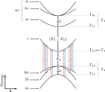
Figure 1: A schematic diagram of the fourteen-band model, indicating band abbreviations (left), energies (center), symmetry of the $\Gamma$-point states (right), and one- and two-photon transitions. $\Gamma_{6}$, $\Gamma_{7}$, and $\Gamma_{8}$ indicate irreducible representations of the $T_{d}$ double group, whereas $\Gamma_{1}$ and $\Gamma_{4}$ indicate irreducible representations of the $T_{d}$ point group. Note that spin-splitting, nonparabolicity, and warping are not shown in this diagram.

The one-electron field-free Hamiltonian is $H=H_{0}+H_{SO}$, where $H_{0}=p^{2}/\left(2m\right)+V$, the potential $V\left(\mathbf{r}\right)$ has the symmetry of the crystal, and the spin-orbit interaction $H_{SO}$ is

$$H_{SO}=\frac{\hbar}{4m^{2}c^{2}}\bm{\sigma}\cdot\left(\bm{\nabla}V\times\mathbf{p}\right),$$

where $\bm{\sigma}$ is the dimensionless spin operator, $\bm{\sigma}=2\mathbf{S}/\hbar$. Note that relativistic corrections proportional to $\left|\bm{\sigma}\times\bm{\nabla}V\right|^{2}$ have been neglected Lax (2001). The eigenstates of $H$ are Bloch states $\left|n\mathbf{k}\right\rangle$ with energy $\hbar\omega_{n}\left(\mathbf{k}\right)$. The associated spinor wave function $\phi_{n\mathbf{k}}\left(\mathbf{r}\right)\equiv\langle\mathbf{r}|n\mathbf{k}\rangle$ can be written $\phi_{n\mathbf{k}}\left(\mathbf{r}\right)=u_{n\mathbf{k}}\left(\mathbf{r}\right)\exp\left(i\mathbf{k}\cdot\mathbf{r}\right)$, where the spinor functions $u_{n\mathbf{k}}\left(\mathbf{r}\right)$ have the periodicity of the crystal lattice. We use the notation $\left|\overline{n\mathbf{k}}\right\rangle$ to denote the kets for the $u$-functions; i.e. $u_{n\mathbf{k}}\left(\mathbf{r}\right)=\langle\mathbf{r}|\overline{n\mathbf{k}}\rangle$. Note that $\left|\overline{n\mathbf{k}}\right\rangle=\exp{\left(-i\mathbf{k}\cdot\mathbf{r}\right)}\left|n\mathbf{k}\right\rangle$. The Hamiltonian for the $u$-function kets, known as the $\mathbf{k}\cdot\mathbf{p}$ Hamiltonian, is Lax (2001); Yu and Cardona (1996)

$$H_{\mathbf{k}}=e^{-i\mathbf{k}\cdot\mathbf{r}}He^{i\mathbf{k}\cdot\mathbf{r}}=H+\frac{\hbar^{2}k^{2}}{2m}+\hbar\mathbf{k}\cdot\mathbf{v},$$

where the velocity operator $\mathbf{v}\equiv\left(i/\hbar\right)\left[H,\mathbf{r}\right]$ is

$$\mathbf{v}=\frac{1}{m}\mathbf{p}+\frac{\hbar}{4m^{2}c^{2}}\left(\bm{\sigma}\times\bm{\nabla}V\right).$$ (2)

The second term in $\mathbf{v}$, the anomalous velocity, which leads to $\mathbf{k}$-dependent spin-orbit coupling in $H_{\mathbf{k}}$, can be neglected for the processes we consider as shown in Appendix A; in the rest of this article, we assume that it vanishes.

The states $\left|n,\mathbf{k=\mathbf{0}}\right\rangle$ are a complete set of eigenstates for the Hamiltonian $H$ on the space of cell-periodic functions. Thus cell-periodic eigenstates of $H_{\mathbf{k}}$ can be expanded in the infinite set of states $\left|n,\mathbf{k=\mathbf{0}}\right\rangle$. The “bare” fourteen-band model truncates this expansion to a set of fourteen states, corresponding to the fourteen bands closest in energy to the fundamental band gap at the $\Gamma$ point Pfeffer and Zawadzki (1990).

In a semiconductor of zinc-blende symmetry, the states $\left\{\left|n,\mathbf{k=\mathbf{0}}\right\rangle|n=1..14\right\}$ are conveniently expanded in the eigenstates of $H_{0}$, $\left\{\left|S\right\rangle,\left|X\right\rangle,\left|Y\right\rangle,\left|Z\right\rangle,\left|x\right\rangle,\left|y\right\rangle,\left|z\right\rangle\right\}\otimes\left\{\left|\uparrow\right\rangle,\left|\downarrow\right\rangle\right\}$, where, under the point group $T_{d}$, $\left|S\right\rangle$ transforms like $\Gamma_{1}$, $\left\{\left|X\right\rangle,\left|Y\right\rangle,\left|Z\right\rangle\right\}$ and $\left\{\left|x\right\rangle,\left|y\right\rangle,\left|z\right\rangle\right\}$ transform like $\Gamma_{4}$ Yu and Cardona (1996). The $\left\{\left|\uparrow\right\rangle,\left|\downarrow\right\rangle\right\}$ comprises the usual spin $1/2$ states:

$$\left\langle\uparrow\right|\bm{\sigma}\left|\uparrow\right\rangle =-\left\langle\downarrow\right|\bm{\sigma}\left|\downarrow\right\rangle=\mathbf{\hat{z}}$$ (3a)

$$\left\langle\uparrow\right|\bm{\sigma}\left|\downarrow\right\rangle =\left(\left\langle\downarrow\right|\bm{\sigma}\left|\uparrow\right\rangle\right)^{*}=\mathbf{\hat{x}}-i\mathbf{\hat{y}}.$$ (3b)

The non-zero matrix elements of $\left(\bm{\nabla}V\times\mathbf{p}\right)$ are

$$\left\langle X\right|\left(\bm{\nabla}V\times\mathbf{p}\right)^{y}\left|Z\right\rangle \equiv i\frac{4m^{2}c^{2}}{3\hbar}\Delta_{0},$$

$$\left\langle x\right|\left(\bm{\nabla}V\times\mathbf{p}\right)^{y}\left|z\right\rangle \equiv i\frac{4m^{2}c^{2}}{3\hbar}\Delta_{0}^{\prime},$$

$$\left\langle X\right|\left(\bm{\nabla}V\times\mathbf{p}\right)^{y}\left|z\right\rangle \equiv i\frac{4m^{2}c^{2}}{3\hbar}\Delta^{-},$$

cyclic permutations of these [e.g. $\left\langle x\right|\left(\bm{\nabla}V\times\mathbf{p}\right)^{y}\left|z\right\rangle=\left\langle z\right|\left(\bm{\nabla}V\times\mathbf{p}\right)^{x}\left|y\right\rangle=\left\langle y\right|\left(\bm{\nabla}V\times\mathbf{p}\right)^{z}\left|x\right\rangle$], and those generated by Hermitian conjugation of these. The above equations define the spin-orbit energies $\Delta_{0}$ and $\Delta_{0}^{\prime}$, and the interband spin-orbit coupling $\Delta^{-}$ Cardona et al. (1965, 1988). The fourteen basis states $\left\{\left|n,\mathbf{k=\mathbf{0}}\right\rangle|n=1..14\right\}$ for $H_{14}$ are

$$\left|\Gamma_{7v},\pm 1/2\right\rangle =\pm\frac{1}{\sqrt{3}}\left|Z\right\rangle\left|\alpha_{\pm}\right\rangle+\frac{1}{\sqrt{3}}\left|X\pm iY\right\rangle\left|\alpha_{\mp}\right\rangle$$ (4a)

$$\left|\Gamma_{8v},\pm 1/2\right\rangle =\mp\sqrt{\frac{2}{3}}\left|Z\right\rangle\left|\alpha_{\pm}\right\rangle+\frac{1}{\sqrt{6}}\left|X\pm iY\right\rangle\left|\alpha_{\mp}\right\rangle$$ (4b)

$$\left|\Gamma_{8v},\pm 3/2\right\rangle =\pm\frac{1}{\sqrt{2}}\left|X\pm iY\right\rangle\left|\alpha_{\pm}\right\rangle$$ (4c)

$$\left|\Gamma_{6c},\pm 1/2\right\rangle =i\left|S\right\rangle\left|\alpha_{\pm}\right\rangle$$ (4d)

$$\left|\Gamma_{7c},\pm 1/2\right\rangle =\pm\frac{1}{\sqrt{3}}\left|z\right\rangle\left|\alpha_{\pm}\right\rangle+\frac{1}{\sqrt{3}}\left|x\pm iy\right\rangle\left|\alpha_{\mp}\right\rangle$$ (4e)

$$\left|\Gamma_{8c},\pm 1/2\right\rangle =\mp\sqrt{\frac{2}{3}}\left|z\right\rangle\left|\alpha_{\pm}\right\rangle+\frac{1}{\sqrt{6}}\left|x\pm iy\right\rangle\left|\alpha_{\mp}\right\rangle$$ (4f)

$$\left|\Gamma_{8c},\pm 3/2\right\rangle =\pm\frac{1}{\sqrt{2}}\left|x\pm iy\right\rangle\left|\alpha_{\pm}\right\rangle,$$ (4g)

where $\left|\alpha_{+}\right\rangle=\left|\uparrow\right\rangle$ and $\left|\alpha_{-}\right\rangle=\left|\downarrow\right\rangle$. The states are labeled with their transformation property under the double group for $T_{d}$, and with a pseudo-angular momentum notation. In the basis (4), $H_{\mathbf{k}=\mathbf{0}}$ is diagonal except for terms proportional to $\Delta^{-}$. The connection between the eigenvalues of $H_{\mathbf{k}=\mathbf{0}}$ for the $\Gamma$-point eigenstates and the eigenvalues of $H_{0}$ is given by Pfeffer and Zawadski Pfeffer and Zawadzki (1990). The nonzero matrix elements of momentum, which appear in $H_{\mathbf{k}}$, are

$$\left\langle S\right|p^{x}\left|X\right\rangle =\left\langle S\right|p^{y}\left|Y\right\rangle=\left\langle S\right|p^{z}\left|Z\right\rangle\equiv imP_{0}/\hbar$$ (5a)

$$\left\langle S\right|p^{x}\left|x\right\rangle =\left\langle S\right|p^{y}\left|y\right\rangle=\left\langle S\right|p^{z}\left|z\right\rangle\equiv imP_{0}^{\prime}/\hbar$$ (5b)

$$\begin{split}\left\langle X\right|p^{y}\left|z\right\rangle&=\left\langle Y\right|p^{z}\left|x\right\rangle=\left\langle Z\right|p^{x}\left|y\right\rangle=\left\langle Z\right|p^{y}\left|x\right\rangle\\ &=\left\langle Y\right|p^{x}\left|z\right\rangle=\left\langle X\right|p^{z}\left|y\right\rangle\equiv imQ/\hbar.\end{split}$$ (5c)

Eq. (5) defines the parameters $P_{0}$, $P_{0}^{\prime}$, and $Q$. They are sometimes expressed as energies $E_{P}$, $E_{P^{\prime}}$, and $E_{Q}$ with the connections $E_{P}=2mP_{0}^{2}/\hbar^{2}$, etc.

The “bare” fourteen-band model has eight empirical parameters $E_{g}$, $\Delta_{0}$, $E_{0}^{\prime}$, $\Delta_{0}^{\prime}$, $\Delta^{-}$, $P_{0}$, $Q$, and $P_{0}^{\prime}$. Its quantitative accuracy is improved by adding important remote band effects to order $k^{2}$ using Löwdin perturbation theory Löwdin (1951), which adds $\mathbf{k}$-dependent terms to the truncated $14\times 14$ Hamiltonian so that its solutions better approximate those of the full Hamiltonian Pfeffer and Zawadzki (1996). The remote band effects are governed by the parameters $\gamma_{1}$, $\gamma_{2}$, $\gamma_{3}$, $F$, and $C_{k}$. The parameters $\gamma_{1}$, $\gamma_{2}$, and $\gamma_{3}$ are modified Luttinger parameters that account for remote band effects on the valence bands. They are related to the usual Luttinger parameters $\gamma_{1L}$, $\gamma_{2L}$, and $\gamma_{3L}$ by the couplings with $\Gamma_{6c}$, $\Gamma_{7c}$, and $\Gamma_{8c}$ bands, which are already accounted for in the “bare” fourteen-band model Pfeffer and Zawadzki (1996):

$$\gamma_{1} =\gamma_{1L}-\frac{E_{P}}{3E_{g}}-\frac{E_{Q}}{3E_{0}^{\prime}}-\frac{E_{Q}}{3E_{0}^{\prime}+\Delta_{0}^{\prime}},$$

$$\gamma_{2} =\gamma_{2L}-\frac{E_{P}}{6E_{g}}+\frac{E_{Q}}{6E_{0}^{\prime}},$$

$$\gamma_{3} =\gamma_{3L}-\frac{E_{P}}{6E_{g}}-\frac{E_{Q}}{6E_{0}^{\prime}}.$$

The parameter $F$ accounts for remote band effects on the lowest conduction band, essentially fixing its effective mass to the experimentally observed value. Finally, the parameter $C_{k}$ is the small $\mathbf{k}$-linear term in the valence bands Cardona et al. (1988). The remote band effects can be removed by setting $\gamma_{1}=-1$ and $\gamma_{2}=\gamma_{3}=F=C_{k}=0$. The model includes neither remote band effects on the $uc$ bands, nor remote band effects on the $\Gamma_{6c}$-$\Gamma_{8v}$ and $\Gamma_{6c}$-$\Gamma_{7v}$ momentum matrix elements, although such terms exist in principle Winkler (2003).

In summary, $H_{14}$ is a fourteen-band approximation to $H_{\mathbf{k}}$ that incorporates some remote band effects. It can be found in Eq. (5) of Pfeffer and Zawadzki, although with a slightly different notation Pfeffer and Zawadzki (1996). With their notation on the left, and ours on the right: $E_{0}=-E_{g}$, $E_{1}=E_{0}^{\prime}-E_{g}$, $\Delta_{1}=\Delta_{0}^{\prime}$, $\overline{\Delta}=\Delta^{-}$, $P_{1}=P_{0}^{\prime}$. Also, our $\Delta_{0}$ differs from theirs by a minus sign. Other authors have also used different notations Winkler (2003). The fourteen bands are shown schematically in Fig. 1 along with the symmetry notation of the $\Gamma$-point states, and the notation used to label the bands.

II.1 Material parameters

Numerical values for the thirteen parameters of the model are listed in Table 1 for InSb, GaSb, InP, GaAs, and ZnSe. They are taken from the literature, where they were chosen to fit low-temperature experimental data. Of the two parameter sets discussed by Pfeffer and Zawadzki for GaAs, we use the one corresponding to $\alpha=0.085$ that they find yields better results Pfeffer and Zawadzki (1996). For InP, GaSb, and InSb, we use parameters from Cardona, Christensen and Fasal Cardona et al. (1988). For cubic ZnSe, we use the parameters given by Mayer and Rossler Mayer and Rössler (1993), we use a calculated value of $C_{k}$ Cardona et al. (1988), and we use $\Delta^{-}=-0.238$ eV to give a $k^{3}$ conduction band spin-splitting that matches the ab initio calculation of Cardona, Christensen and Fasal Cardona et al. (1988). Winkler used these same parameters for ZnSe, but took $\Delta^{-}=0$ Winkler (2003). There is more uncertainty in the parameters for ZnSe than in those for the other materials Mayer and Rössler (1993), but we include it as an example of a semiconductor with a larger band gap.

Table 1: Model parameters.

	GaAs	InP	GaSb	InSb	ZnSe
$E_{g}$ (eV)	$1.519$	$1.424$	$0.813$	$0.235$	$2.820$
$\Delta_{0}$ (eV)	$0.341$	$0.108$	$0.75$	$0.803$	$0.403$
$E_{0}^{\prime}$ (eV)	$4.488$	$4.6$	$3.3$	$3.39$	$7.330$
$\Delta_{0}^{\prime}$ (eV)	$0.171$	$0.50$	$0.33$	$0.39$	$0.090$
$\Delta^{-}$ (eV)	$-0.061$	$0.22$	$-0.28$	$-0.244$	$-0.238$
$P_{0}$ (eVÅ)	$10.30$	$8.65$	$9.50$	$9.51$	$10.628$
$Q$ (eVÅ)	$7.70$	$7.24$	$8.12$	$8.22$	$9.845$
$P_{0}^{\prime}$ (eVÅ)	$3.00$	$4.30$	$3.33$	$3.17$	$9.165$
$\gamma_{1L}$	$7.797$	$5.05$	$13.2$	$40.1$	$4.30$
$\gamma_{2L}$	$2.458$	$1.6$	$4.4$	$18.1$	$1.14$
$\gamma_{3L}$	$3.299$	$1.73$	$5.7$	$19.2$	$1.84$
$F$	$-1.055$	$0$	$0$	$0$	$0$
$C_{k}$ (meVÅ)	$-3.4$	$-14$	$0.43$	$-9.2$	$-14$

The parabolic-band approximation calculations use parameters from Table 1, and average effective masses derived from the parameters in Table 1.

II.2 Matrix elements

The relations between matrix elements of the Bloch states and matrrix elements of the $u$-function kets are

$$\mathbf{v}_{nm}\left(\mathbf{k}\right)\equiv\left\langle n\mathbf{k}\right|\mathbf{v}\left|m\mathbf{k}\right\rangle=\left\langle\overline{n\mathbf{k}}\right|\mathbf{v}\left|\overline{m\mathbf{k}}\right\rangle+\frac{\hbar\mathbf{k}}{m}\delta_{nm},$$ (6)

$$\left\langle n\mathbf{k}\right|\mathbf{S}\left|m\mathbf{k}\right\rangle=\left\langle\overline{n\mathbf{k}}\right|\mathbf{S}\left|\overline{m\mathbf{k}}\right\rangle$$ (7)

$$\left\langle n\mathbf{k}\right|v^{i}S^{j}\left|m\mathbf{k}\right\rangle=\left\langle\overline{n\mathbf{k}}\right|v^{i}S^{j}\left|\overline{m\mathbf{k}}\right\rangle+\frac{\hbar k^{i}}{m}\left\langle\overline{n\mathbf{k}}\right|S^{j}\left|\overline{m\mathbf{k}}\right\rangle.$$ (8)

The matrix elements of the velocity operator, $\mathbf{v}$, neglecting the anomalous velocity as discussed in Appendix A, can be calculated using (2), (5), and the right side of (6). The matrix elements of the spin operator $\mathbf{S}$, can be found from Eq. (3). The matrix elements of $v^{i}S^{j}$ can be similarly found in the basis of eigenstates of $H_{0}$. Each of these can then be rotated to the basis (4) in which the states $\left|\overline{m\mathbf{k}}\right\rangle$ are expanded.

It is well known that, in a crystal, $\mathbf{v}_{nn}\left(\mathbf{k}\right)=\nabla_{\mathbf{k}}\omega_{n}\left(\mathbf{k}\right)$. More generally,

$$\mathbf{v}_{nm}\left(\mathbf{k}\right)=\nabla_{\mathbf{k}}\left\langle n\mathbf{k}\right|H\left|m\mathbf{k}\right\rangle=\left\langle\overline{n\mathbf{k}}\right|\nabla_{\mathbf{k}}H_{\mathbf{k}}\left|\overline{m\mathbf{k}}\right\rangle.$$ (9)

These identities can be proven from the definitions $H_{\mathbf{k}}=e^{-i\mathbf{k}\cdot\mathbf{r}}He^{i\mathbf{k}\cdot\mathbf{r}}$ and $\mathbf{v}=\left(i/\hbar\right)\left[H,\mathbf{r}\right]$, even for a non-local Hamiltonian. But when remote band effects are included in a finite band model, they no longer hold. That is, $\mathbf{v}_{nm}\left(\mathbf{k}\right)$ calculated using (6) and eigenstates of $H_{14}$ is not equal to $\left\langle\overline{n\mathbf{k}}\right|\nabla_{\mathbf{k}}H_{14}\left|\overline{m\mathbf{k}}\right\rangle$. We explicitly restore these identities by using $\left\langle\overline{n\mathbf{k}}\right|\nabla_{\mathbf{k}}H_{14}\left|\overline{m\mathbf{k}}\right\rangle$ to calculate $\mathbf{v}_{nm}\left(\mathbf{k}\right)$. This approach can be described as including remote band effects in the velocity operator. It was used for an eight band calculation of linear absorption by Enders et al Enders et al. (1995). This step is not critically important for the effects calculated here, since remote band effects are generally small.

II.3 $\mathbf{k}$-space integration

The optical calculations in this article have the form $\Theta$, where

$$\Theta=\sum_{c,v}\int d^{3}kf_{cv}\left(H_{\mathbf{k}}\right)\delta\left(\hbar\omega_{cv}\left(\mathbf{k}\right)-2\hbar\omega\right),$$ (10)

where $f_{cv}$ depends on matrix elements and energies of eigenstates of $H_{\mathbf{k}}$, and where $\omega_{nm}\left(\mathbf{k}\right)\equiv\omega_{n}\left(\mathbf{k}\right)-\omega_{m}\left(\mathbf{k}\right)$. The integral in (10) is understood to be restricted to the first Brillioun Zone, but we do not actively enforce the restriction, since the photon energies considered here cause transitions well within the first Brillioun Zone. Writing $\mathbf{k}=\left(k_{cv},\theta_{\mathbf{k}},\phi_{\mathbf{k}}\right)$ in spherical coordinates, where $k_{cv}$ is the solution to

$$\hbar\omega_{cv}\left(k_{cv},\theta_{\mathbf{k}},\phi_{\mathbf{k}}\right)-2\hbar\omega=0,$$ (11)

we have

$$\Theta=8\sum_{c,v}\int_{0}^{\pi/2}\int_{0}^{\pi/2}\frac{k_{cv}^{2}\sin\theta_{\mathbf{k}}f_{cv}\left(H_{\mathbf{k}}\right)}{\left|\hbar\left(\mathbf{v}_{cc}\left(\mathbf{k}\right)-\mathbf{v}_{vv}\left(\mathbf{k}\right)\right)\cdot\mathbf{\hat{k}}\right|}d\phi_{\mathbf{k}}d\theta_{\mathbf{k}},$$ (12)

where we have used $\bm{\nabla}\omega_{n}\left(\mathbf{k}\right)=\mathbf{v}_{nn}\left(\mathbf{k}\right)$ and the cubic symmetry of the crystal. It is numerically convenient to do the sum over any degenerate bands before the integral over $\theta_{\mathbf{k}}$ and $\phi_{\mathbf{k}}$.

II.4 Approximations

The calculations of “1+2” effects in the following sections are primarily labeled by the Hamiltonian used to approximate $H_{\mathbf{k}}$. The complete fourteen-band model is denoted $H_{14}$. The bare fourteen-band model, denoted $H_{14\text{-Bare}}$, is $H_{14}$ without remote band effects. The $8\times 8$ subset of the fourteen band Hamiltonian within the basis $\left\{\Gamma_{6c},\Gamma_{8v},\Gamma_{7v}\right\}$ is denoted $H_{8}$. The spherical eight-band model, denoted $H_{8\text{Sph}}$, is derived from $H_{8}$ by setting $C_{k}=0$ and replacing $\gamma_{2}$ and $\gamma_{3}$ by $\tilde{\gamma}\equiv\left(2\gamma_{2}+3\gamma_{3}\right)/5$;Baldereschi and Lipari (1973) it is a spherical approximation to the Kane model including remote band effects Kane (1957). The aforementioned calculations are non-perturbative in $\mathbf{k}$; that is, in each case, the Hamiltonian is solved numerically at each $\mathbf{k}$. The perturbative calculations of Appendix B are denoted PBA (parabolic-band approximation).

The microscopic expression for each of the “1+2” effects contains a sum over intermediate bands, which originates from the two-photon amplitude. Unless otherwise noted, calculations include all possible intermediate bands (eg., $H_{14}$ includes fourteen intermediate bands, and $H_{8\text{Sph}}$ includes eight intermediate bands). Calculations that restrict this sum are secondarily labeled to reflect the restriction. The label “$H_{14}$, no $uc$” uses $H_{14}$, but does not include $uc$ bands as intermediate states. The label “$H_{14}$, no $uc$/$so$” uses $H_{14}$, but includes neither $uc$ nor $so$ bands as intermediate states. The label “$H_{14}$, 2BT” uses $H_{14}$, but only includes two-band terms (terms for which the intermediate band is the same as the initial or final band). Similar labels are used for $H_{8\text{Sph}}$, for example, “$H_{8\text{Sph}}$-PBA, no so” uses the perturbative solution to $H_{8\text{Sph}}$ and does not include $so$ intermediate states.

III Current

The current injection rate due to the field (1) can be written

$$\dot{J}^{i}=\eta_{\left(1\right)}^{ijk}E_{2\omega}^{j*}E_{2\omega}^{k}+\dot{J}_{(I)}^{i}+\eta_{\left(2\right)}^{ijklm}E_{\omega}^{j*}E_{\omega}^{k*}E_{\omega}^{l}E_{\omega}^{m},$$ (13)

where $\mathbf{J}$ is the macroscopic current density, and

$$\dot{J}_{(I)}^{i}=\eta_{(I)}^{ijkl}E_{\omega}^{j*}E_{\omega}^{k*}E_{2\omega}^{l}+c.c.$$ (14)

The third rank tensor $\eta_{\left(1\right)}^{ijk}$ describes one-photon current injection (the circular photogalvanic effect Sturman and Fridkin (1992); Ganichev and Prettl (2003)), the fifth rank tensor $\eta_{\left(2\right)}^{ijklm}$ describes two-photon current injection, and the fourth rank tensor $\eta_{(I)}^{ijkl}$ describes “1+2” current injection Atanasov et al. (1996). Aversa and Sipe showed that $\eta_{(I)}^{ijkl}$ is related to a doubly divergent part of the third-order nonlinear susceptibility $\chi^{\left(3\right)}$ Aversa and Sipe (1996). In cubic materials with point group symmetry $T_{d}$, $O_{h}$ or $O$, a general fourth rank tensor has four independent components, but due to the intrinsic symmetry $\eta_{(I)}^{ikjl}=\eta_{(I)}^{ijkl}$, $\eta_{(I)}$ has only three independent components; there are 21 non-zero components of $\eta_{(I)}$ in the standard cubic basis: $\eta_{(I)}^{aaaa}=\eta_{(I)}^{bbbb}=\eta_{(I)}^{cccc}$, $\eta_{(I)}^{baab}=\eta_{(I)}^{abba}=\eta_{(I)}^{caac}=\eta_{(I)}^{acca}=\eta_{(I)}^{cbbc}=\eta_{(I)}^{bccb}$, and $\eta_{(I)}^{a\left(ab\right)b}=\eta_{(I)}^{b\left(bc\right)c}=\eta_{(I)}^{c\left(ca\right)a}=\eta_{(I)}^{a\left(ac\right)c}=\eta_{(I)}^{c\left(cb\right)b}=\eta_{(I)}^{b\left(ba\right)a}$ (the components in parentheses can be exchanged), where $a$, $b$, and $c$ denote components along the principal cubic axes Atanasov et al. (1996). This can be written

$$\eta_{(I)}^{ijkl}=i\frac{\eta_{B1}}{2}\left(\delta^{ij}\delta^{kl}+\delta^{ik}\delta^{jl}\right)+i\eta_{B2}\delta^{il}\delta^{jk}+i\eta_{C}\delta^{ijkl},$$ (15)

where $\delta^{ij}$ is a Kronecker delta and the only non-isotropic part is $\delta^{ijkl}$, which we define in the principal cubic basis as $\delta^{ijkl}=1$ when $i=j=k=l$ and zero otherwise. The three independent components are $\eta_{B1}\equiv-2i\eta^{aabb}$, $\eta_{B2}\equiv-i\eta^{abba}$, and $\eta_{C}\equiv 2i\eta^{aabb}+i\eta^{abba}-i\eta^{aaaa}$. Thus, in a cubic material,

$$\begin{split}\dot{J}_{(I)}^{i}=&i\eta_{B1}\left(\mathbf{E}_{\omega}^{*}\cdot\mathbf{E}_{2\omega}\right)E_{\omega}^{i*}+i\eta_{B2}\left(\mathbf{E}_{\omega}\cdot\mathbf{E}_{\omega}\right)^{*}E_{2\omega}^{i}\\ &+i\eta_{C}\delta^{ijkl}E_{\omega}^{j*}E_{\omega}^{k*}E_{2\omega}^{l}+c.c.\end{split}$$ (16)

This generalizes the notation we used previously for a calculation in the parabolic-band approximation Bhat and Sipe (2000), with the connection $\eta_{B1}=eDB_{1}/\hbar$, and $\eta_{B2}=eDB_{2}/\hbar$. In that, or any other spherical approximation, $\eta_{C}=0$.

To calculate $\eta_{(I)}$, we use the microscopic expression first given by Atanasov et al. Atanasov et al. (1996), modified to explicitly include the sum over spin states van Driel and Sipe (2001); Najmaie et al. (2003). An alternate microscopic expression has been derived in the length gauge Aversa and Sipe (1996), but it has not yet been used in a calculation. In the independent particle approximation that we employ here, $\eta_{(I)}$ is purely imaginary Atanasov et al. (1996) and hence $\eta_{B1}$, $\eta_{B2}$, and $\eta_{C}$ are real, although they can be complex if excitonic effects are included Bhat and Sipe (2005).

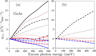
Figure 2: (color online): Spectra of $\eta_{B1}$ (black lines), $\eta_{B2}$ (red lines), and $\eta_{C}$ (blue lines) for GaAs. Panel (a) shows the contributions from each initial valence band; dashed, dotted, and dashed-dotted lines include only transitions from the $hh$, $lh$, and $so$ bands respectively, while the solid lines include all three transitions. The thin solid, light brown line in (a) is the total $\mathrm{Re}\left(\eta_{(I)}^{aaaa}\right)$. Panel (b) separates the total into electron (dashed) and hole (dotted) contributions.

The spectra of $\eta_{B1}$, $\eta_{B2}$, and $\eta_{C}$, calculated for GaAs, are shown in Fig. 2(a) along with the contributions to each tensor component from each possible initial valence band. For a given photon energy, electrons photoexcited from the $hh$ band have higher energies and velocities than electrons photoexcited from the $lh$ band; hence the dominant component $\eta_{B1}$ is larger for $hh$-$c$ transitions than $lh$-$c$ transitions. The smallness of $\eta_{B2}$ is due to contributions from the $hh$-$c$ transitions having opposite sign to the $lh$-$c$ transitions, as shown previously in the PBA Bhat and Sipe (2000).

Figure 2(b) separates each tensor component into an electron contribution and a hole contribution (denoted $\eta_{e}$ and $\eta_{h}$ by Atanasov et al Atanasov et al. (1996)). Electrons make a larger contribution to $\eta_{B1}$ than holes, due to the lower effective mass (and hence higher velocity) of an electron than of a hole (much lower, in the case of a heavy hole) with the same crystal momentum. Holes dominate $\eta_{B2}$ at lower photon energies, while electrons dominate $\eta_{B2}$ at higher energies. Both electrons and holes contribute equally to the anisotropic component $\eta_{C}$.

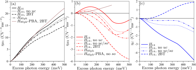
Figure 3: (color online): Approximations for GaAs current injection tensor components (a) $\eta_{B1}$, (b) $\eta_{B2}$, and (c) $\eta_{C}$. The approximations are described in Sec. II.4.

To help in understanding the importance of the various intermediate states, in Fig. 3 we compare the calculated current injection tensor elements with various degrees of approximation described in Sec. II.4.

The component $\eta_{B1}$ (and hence $\eta_{(I)}^{aaaa}$, since $\eta_{B1}$ is larger than $\eta_{B2}+\eta_{C}$) is dominated by two-band terms. Three-band terms cause an increase, by as much as 34%, of $\eta_{B1}$ [the difference between the dashed and solid black lines in Fig. 3(a)]. Although not shown in Fig. 3, most of the increase is due to three-band terms with the $so$ band as an intermediate state. Terms with the $uc$ bands as intermediate states only cause a small increase to $\eta_{B1}$ (the difference between the dotted and solid black lines). The warping of the bands is clearly not important for $\eta_{B1}$, since the calculation with $H_{8\text{Sph}}$ closely approximates the calculation “$H_{14}$, no $uc$”, which includes the same intermediate states. Surprisingly, the “$H_{8\text{Sph}}$-PBA, 2BT” result Bhat and Sipe (2000, 2005) closely approximates the complete, non-perturbative fourteen-band calculation, even at excess photon energies for which band nonparabolicity is significant. This is due to a fortuitous compensation between the neglect of nonparabolicity and the neglect of three-band terms. The compensation is not as complete for all materials.

The component $\eta_{B2}$, which determines the current due to orthogonal linearly polarized fields, is less forgiving to approximations than the component $\eta_{B1}$. We have already seen in Fig. 2 that $\eta_{B2}$ is small due to a near cancellation of $hh$ and $lh$ initial states. Reasonable accuracy on $\eta_{B2}$ thus requires higher accuracy on the contribution from each initial state. In particular, three-band terms must not be neglected. By comparing the dashed-dotted and solid lines in Fig. 3(b), it can be seen that, whereas the sum of the two-band terms is negative, the sum of the three-band terms is positive and of the same magnitude. It is useful to divide the three-band terms into three groups: those with intermediate state from the $hh$ or $lh$ bands, those with intermediate state from the $so$ band, and those with intermediate state from one of the $uc$ bands. We find that each group contributes roughly the same positive amount to $\eta_{B2}$ for excess photon energies less than $\Delta_{0}$. The groups are added successively to the 2BTs in the dashed, dotted, and solid lines in Fig. 3(b). Three-band terms with $so$ intermediate states are less important at the higher excess photon energies in Fig. 3(b). The warping of the bands makes a small but non-negligible contribution to $\eta_{B2}$, as seen in the difference between the dashed-double-dotted and dotted lines of Fig. 3(b). The solid brown line in Fig. 3(b) is the “$H_{8\text{Sph}}$-PBA, no $so$” result Bhat and Sipe (2000). At low excess photon energies, it greatly underestimates $\eta_{B2}$ due to the neglect of $so$ and $uc$ intermediate states, while at excess photon energies greater than 100 meV, this is partly compensated for by the neglect of nonparabolicity. It appears from the difference between “$H_{8\text{Sph}}$-PBA, no $so$” and “$H_{14}$, no $uc$/$so$” in Fig. 3(b) that nonparabolicity becomes important at energies above 70 meV.

The term $\eta_{C}$ is purely due to cubic anisotropy by definition; in any model that is spherically symmetric it is identically zero. There is no cubic anisotropy in the “bare” (i.e. without remote band effects) eight-band model on the set $\left\{\Gamma_{6c},\Gamma_{8v},\Gamma_{7v}\right\}$. Cubic anisotropy in the fourteen-band model is due to the momentum matrix elements governed by the parameters $E_{Q}$ and $E_{P^{\prime}}$, the interband spin-orbit coupling $\Delta^{-}$, and remote bands through $(\gamma_{2}-\gamma_{3})$ and $C_{k}$. From Fig. 3(c), it can be seen that three-band terms are important for $\eta_{C}$. In fact, with only 2BTs included, $\eta_{C}$ is positive for GaAs, whereas it is negative with all terms included. From Fig. 3(c) it can also be seen that the $so$ band and $uc$ bands are important as intermediate states for $\eta_{C}$.

Our calculation of $\eta_{(I)}$ is of the same order of magnitude as the ab initio calculation of Atanasov et al. Atanasov et al. (1996), but its spectral dependence is different. In particular, $\eta_{B1}$ agrees more closely with the PBA calculation, as seen in Fig. 3(a). Atanasov et al. had attributed the difference between their ab initio and PBA calculations to the assumption of $\mathbf{k}$-independent velocity matrix elements in the PBA Atanasov et al. (1996). However, our calculation accounts for the $\mathbf{k}$-dependence of velocity matrix elements and agrees closely (for $\eta_{B1}$ and $\mathrm{Re}\eta^{aaaa}$) to the PBA. The earlier ab initio calculation Atanasov et al. (1996) was, in fact, inaccurate at low photon energies due to various computational issues; an improved ab initio calculation agrees with the spectral dependence at low photon energy given here Nastos .

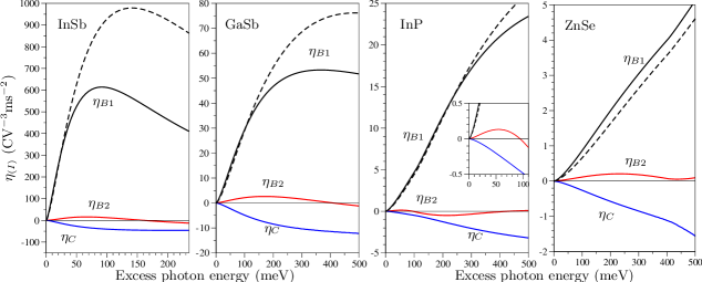
Figure 4: (color online): $\eta_{B1}$ (black), $\eta_{B2}$ (red), and $\eta_{C}$ (blue) for (a) InSb, (b) GaSb, (c) InP, and (d) ZnSe. The solid lines are calculated with the complete fourteen-band model. The dashed line for $\eta_{B1}$ is “$H_{8\text{Sph}}$-PBA, 2BT” Bhat and Sipe (2000, 2005). The inset of panel (c) shows the area near the origin in more detail.

Figure 4 shows the spectra of $\eta_{B1}$, $\eta_{B2}$, and $\eta_{C}$ calculated with $H_{14}$ for InSb, GaSb, InP, and ZnSe. The dashed black line in Fig. 4 is the PBA result Bhat and Sipe (2000, 2005). The PBA appears to be a reasonable approximation to $\eta_{B1}$ for excess energies less than about $0.2E_{g}$. In each material, $\eta_{B2}\ll\eta_{B1}$, and in each material except for ZnSe, the sign of $\eta_{B2}$ varies as a function of frequency. The component $\eta_{C}$, which arises due to cubic anisotropy, is negative for each material.

The cubic anisotropy of current injection due to colinearly polarized fields can be significant enough that it should be measurable. For fields colinearly polarized along $\mathbf{\hat{e}}$, specified by polar angles $\theta$ and $\phi$ relative to the cubic axes,

$$\mathbf{\dot{J}}_{(I)}\cdot\mathbf{\hat{e}}=2\mathrm{Im}\left(E_{\omega}^{2}E_{2\omega}^{*}\right)\left[\eta_{B1}+\eta_{B2}+\eta_{C}-\frac{\eta_{C}}{2}f\left(\theta,\phi\right)\right],$$ (17)

where $f\left(\theta,\phi\right)=\sin^{2}\left(2\theta\right)+\sin^{4}\left(\theta\right)\sin^{2}\left(2\phi\right)$. In general, $\mathbf{\dot{J}}_{(I)}$ also has a component perpendicular to $\mathbf{\hat{e}}$ that is proportional to $\eta_{C}$, but it vanishes for $\mathbf{\hat{e}}$ parallel to $\left\langle 001\right\rangle$, $\left\langle 110\right\rangle$, $\left\langle 111\right\rangle$. The field polarization that maximizes the current injection depends on the relative sign of $\eta_{C}$ and $\mathrm{Re}\eta^{aaaa}=\eta_{B1}+\eta_{B2}+\eta_{C}$. When they have the opposite sign, current injection is a minimum for $\mathbf{\hat{e}\parallel}\left\langle 001\right\rangle$ ($f=0$) and a maximum for $\mathbf{\hat{e}\parallel}\left\langle 111\right\rangle$ ($f=4/3$); for light normally incident on a $\left\{001\right\}$ surface, the largest current injection occurs when $\mathbf{\hat{e}\parallel}\left\langle 110\right\rangle$ ($f=1$). When they have the same sign, current-injection is a maximum for $\mathbf{\hat{e}\parallel}\left\langle 001\right\rangle$ and a minimum for $\mathbf{\hat{e}\parallel}\left\langle 111\right\rangle$. From the GaAs results shown in Fig. 2(a), the current injection for the three cases $\mathbf{\hat{e}\parallel}\left\langle 001\right\rangle$, $\mathbf{\hat{e}\parallel}\left\langle 110\right\rangle$, and $\mathbf{\hat{e}\parallel}\left\langle 111\right\rangle$ are in the ratio 1 to 1.14 to 1.20 at the band edge, 1 to 1.15 to 1.20 at 200 meV excess photon energy, and 1 to 1.22 to 1.29 at 500 meV excess photon energy. In contrast, the ab initio calculation of Atanasov et al. yields larger ratios, for example 1 to 1.32 to 1.43 at 300 meV excess photon energy Atanasov et al. (1996). This disagreement is consistent with the inaccuracy of the ab initio calculation discussed above. Initial experiments with GaAs used $\mathbf{\hat{e}\parallel}\left[001\right]$ Haché et al. (1997); Stevens et al. (2002), whereas Roos et al. exploited the larger signal for $\mathbf{\hat{e}\parallel}\left[110\right]$ Roos et al. (2003). For each of the materials shown in Fig. 4, the minimum current injection is for $\mathbf{\hat{e}\parallel}\left\langle 001\right\rangle$. It is worth noting that two-photon absorption is also a minimum with $\mathbf{\hat{e}\parallel}\left\langle 001\right\rangle$ for many semiconductors Dvorak et al. (1994); Hutchings and Wherrett (1994b); Murayama and Nakayama (1995). It seems that both “1+2” current injection and two-photon absorption with linearly polarized fields are larger for $\mathbf{\hat{e}}$ directed along the bonds.

The cubic anisotropy of “1+2” current injection is pronounced for cross-linearly polarized fields and opposite-circularly polarized fields. For example, for cross-linearly polarized fields normally incident on $\left(001\right)$ with $\mathbf{\hat{e}}_{\omega}=\mathbf{\hat{a}}\cos\phi+\mathbf{\hat{b}}\sin\phi$ and $\mathbf{\hat{e}}_{2\omega}=-\mathbf{\hat{a}}\sin\phi+\mathbf{\hat{b}}\cos\phi$,

$$\begin{split}\mathbf{\dot{J}}_{(I)}=&\mathrm{Im}\left(E_{\omega}^{2}E_{2\omega}^{*}\right)\\ &\times\left[\left(2\eta_{B2}+\eta_{C}\sin^{2}\left(2\phi\right)\right)\mathbf{\hat{e}}_{2\omega}-\frac{\eta_{C}}{2}\sin\left(4\phi\right)\mathbf{\hat{e}}_{\omega}\right].\end{split}$$ (18)

For fields with opposite circular polarizations, the current injection is proportional to $\eta_{C}$ and is hence purely anisotropic.

The component $\eta_{C}$ causes a type of current injection that has not previously been noted. In all “1+2” experiments considered thus far with light normally incident on a surface, the direction of current injection lies in the plane of the surface. However, with co-linearly polarized light fields normally incident on a $\left(111\right)$ surface, the current can have a component into (or out of) the surface. The current in this case is

$$\mathbf{\dot{J}}_{(I)}=2\mathrm{Im}\left(E_{\omega}^{2}E_{2\omega}^{*}\right)\left[\bar{\eta}\mathbf{\hat{e}}+\frac{\sqrt{2}}{6}\eta_{C}\cos\left(3\theta\right)\mathbf{\hat{z}}\right],$$ (19)

where $\bar{\eta}\equiv\left(\eta_{B1}+\eta_{B2}+\frac{1}{2}\eta_{C}\right)$, $\mathbf{\hat{z}}$ is the $\left[111\right]$ direction, and $\theta$ is the angle between $\mathbf{\hat{e}}$ and the $\left[2\bar{1}\bar{1}\right]$ direction. Thus, $\eta_{C}$ governs this “surfacing” current.

IV Population control

The carrier injection rate due to the field (1) can be written $\dot{N}=\dot{N}_{(1)}+\dot{N}_{(I)}+\dot{N}_{(2)}$, where $N$ is the density of electron-hole pairs, $\dot{N}_{(1)}=\xi_{\left(1\right)}^{ij}E_{2\omega}^{i*}E_{2\omega}^{j}$ is one-photon absorption, $\dot{N}_{(2)}=\xi_{\left(2\right)}^{ijkl}E_{\omega}^{i*}E_{\omega}^{j*}E_{\omega}^{k}E_{\omega}^{l}$ is two-photon absorption, and

$$\dot{N}_{(I)}=\xi_{(I)}^{ijk}E_{\omega}^{*i}E_{\omega}^{*j}E_{2\omega}^{k}+c.c.$$ (20)

is “1+2” population control Fraser et al. (1999). The third-rank tensor $\xi_{(I)}^{ijk}$ has intrinsic symmetry $\xi_{(I)}^{jik}=\xi_{(I)}^{ijk}$. In centrosymmetric materials, such as those with the diamond structure (point group $O_{h}$), $\xi_{(I)}^{ijk}$ is identically zero; hence, population control requires a noncentrosymmetric material. In a material with zinc-blende symmetry (point group $T_{d}$), $\xi_{(I)}^{ijk}$ has only one independent component; in the standard cubic basis, $\xi_{(I)}^{abc}=\xi_{(I)}^{cab}=\xi_{(I)}^{bca}=\xi_{(I)}^{acb}=\xi_{(I)}^{bac}=\xi_{(I)}^{cba}$ are the only non-zero components, where $a$, $b$, and $c$ denote components along the principal cubic axes.

We calculate $\xi_{(I)}$ with the microscopic expression given by Fraser et al., which was derived in the independent-particle approximation, and is restricted to $\hbar\omega<E_{g}<2\hbar\omega$ Fraser et al. (1999). Under those conditions, $\xi_{(I)}$ is real and is proportional to the imaginary part of the susceptibility for second harmonic generation (SHG) Fraser et al. (1999); Sipe and Shkrebtii (2000); specifically, (in mks)

$$\xi_{(I)}^{abc}=\frac{2\varepsilon_{0}}{\hbar}\mathrm{Im}\chi^{\left(2\right)cba}\left(-2\omega;\omega,\omega\right).$$ (21)

This connection to SHG, which can be derived from considerations of energy transfer and macroscopic electrodynamics Fraser et al. (1999); Bhat and Sipe (2005), is important because the imaginary part of $\chi^{\left(2\right)}\left(-2\omega;\omega,\omega\right)$ has sometimes been presented en route to a calculation of $\left|\chi^{(2)}\right|$ Bell (1971); Moss et al. (1987); Ghahramani et al. (1991); Huang and Ching (1993); Lew Yan Voon and Ram-Mohan (1994); Hughes and Sipe (1996); Adolph and Bechstedt (1998). As well, analytic expressions have been derived for the dispersion of SHG by using simple band models, with approximations appropriate for $2\hbar\omega$ near the band gap Bell (1971); Kelley (1963a, b); Rustagi (1969); Bell (1972); Jha and Wynne (1972). However, these earlier works did not connect $\mathrm{Im}\chi^{\left(2\right)}\left(-2\omega;\omega,\omega\right)$ with population control, and in fact typically stated that it was not independently observable.

Figure 5: $\mathrm{Im}\chi^{\left(2\right)}$ calculated with $H_{14}$ (solid line) and $H_{14}$-PBA (dashed line) for (a) InSb, (b) GaSb, (c) InP, (d) GaAs, and (e) ZnSe. Panel (f) shows the GaAs calculations on a log-log plot.

Fig. 5 shows the calculation of $\mathrm{Im}\chi^{\left(2\right)cba}\left(-2\omega;\omega,\omega\right)$ for InSb, GaSb, InP, GaAs and ZnSe. Also shown for comparison is the PBA expression (44), derived in Appendix B. Each spectrum can be divided into roughly three regions. At very low excess photon energies, visible in the log-log plot Fig. 5(f), the spectrum is roughly independent of $\omega$. This flat part of the spectrum disappears if $C_{k}$ is set to zero; hence, it is due to the $\mathbf{k}$-linear term in the $c$ band spin-splitting. Next higher in photon energy, up to about 100 meV in GaSb, InP, GaAs, and ZnSe (up to about 15 meV in InSb), is a region where the agreement with the analytic expression (44) is best. In this region, the ratio $X_{2}/X_{1}$, defined in Appendix B, is $0.37$ for InSb, $0.30$ for GaSb, $-0.25$ for InP, $0.08$ for GaAs, and $0.07$ for ZnSe. At higher photon energies, the dispersion of $\mathrm{Im}\chi^{\left(2\right)cba}\left(-2\omega;\omega,\omega\right)$ deviates from the PBA expression due to band nonparabolicity and warping, $\mathbf{k}$-dependence of matrix elements, and transitions from the split-off band, which are not included in (44).

If we remove the two-band transitions $hh$-$\left\{hh,c\right\}$-$c$, $lh$-$\left\{lh,c\right\}$-$c$, and $so$-$\left\{so,c\right\}$-$c$, then the calculation of $\mathrm{Im}\chi^{\left(2\right)}$ (or $\xi_{(I)}$) is unchanged. This is expected for materials of zinc-blende symmetry Kelley (1963b); Aspnes (1972). Further, many years ago Aspnes argued that the so-called “virtual hole terms” of the form $lh$-$\{so,hh\}$-$c$ and $hh$-$\{so,lh\}$-$c$ make only a small contribution to $\chi^{\left(2\right)}\left(0\right)$ Aspnes (1972). Such terms have been neglected in some previous calculations of $\chi^{\left(2\right)}$ dispersion Moss et al. (1987); Huang and Ching (1993). By removing the virtual hole terms, leaving only $\left\{so,lh,hh\right\}$-$uc$-$c$ transitions, we find $\xi_{(I)}$ is reduced by only 6–10% over the range from the band edge to 500 meV above the gap for GaAs. It is thus clear that inclusion of the $uc$ bands is necessary for a calculation of population control. For some purposes it is also sufficient, since if remote band effects are removed from the model, leaving the “bare” fourteen-band model Pfeffer and Zawadzki (1990); Hutchings and Wherrett (1994a), $\xi_{(I)}$ is decreased by only 7–10% from its full value for GaAs.

For most materials, the results in Fig. 5 are in reasonable agreement with previous calculations of $\mathrm{Im}\chi^{\left(2\right)}$ Adolph and Bechstedt (1998); Hughes and Sipe (1996); Huang and Ching (1993); Bell (1971), although most previous calculations had poor spectral resolution in this energy range. However, for ZnSe, the situation is more complicated. The calculation of Huang and Chin is about an order of magnitude smaller than ours Huang and Ching (1993), and that of Ghahramani et al. is about 5 times smaller than ours Ghahramani et al. (1991). Note also that Huang and Chin calculated $\chi^{\left(2\right)}\left(0\right)$ for ZnSe to be an order of magnitude smaller than experimental results Huang and Ching (1993). Wagner et al. have measured the dispersion of $|\chi^{\left(2\right)}|$, which is an upper bound on $\mathrm{Im}\chi^{\left(2\right)}$; for ZnSe it is about a factor of two smaller than our calculation of $\mathrm{Im}\chi^{\left(2\right)}$ Wagner et al. (1998). Note that Wagner et al. give a different set of band parameters than we have used here Wagner et al. (1998).

The magnitude of $\xi_{(I)}^{abc}$ determines the magnitude of population control, but in an experiment one is more interested in the depth of the phase-dependent modulation of the carrier absorption, i.e. the control ratio $R$ Fraser et al. (1999). It is

$$R=\frac{\dot{N}_{(I)}}{\dot{N}_{(1)}+\dot{N}_{(2)}}=\frac{\xi_{(I)}^{ijk}E_{2\omega}^{i*}E_{\omega}^{j}E_{\omega}^{k}+c.c.}{\xi_{(1)}^{ij}E_{2\omega}^{i*}E_{2\omega}^{j}+\xi_{(2)}^{ijkl}E_{\omega}^{i*}E_{\omega}^{j*}E_{\omega}^{k}E_{\omega}^{l}}.$$

This ratio is largest for field amplitudes that equalize $\dot{N}_{(1)}$ and $\dot{N}_{(2)}$ Fraser and van Driel (2003); in what follows, we assume this condition has been met. The ratio then depends only on $\xi_{(I)}^{ijk}$, $\xi_{(1)}^{ij}$, $\xi_{(2)}^{ijkl}$, and the polarizations of the two fields. For light normally incident on a $\left(111\right)$ surface, linearly-polarized fields yield $R=\sqrt{2}\xi_{(I)}^{abc}/\sqrt{3\xi_{(1)}^{aa}\xi_{(2)}^{aaaa}\left(1-\sigma/2\right)}$, while opposite circularly-polarized fields yield

$$R=2\xi_{(I)}/\sqrt{3\xi_{(1)}\xi_{(2)}^{aaaa}\left(1-\sigma/6-\delta\right)},$$ (22)

where $\sigma\equiv(\xi_{(2)}^{aaaa}-\xi_{(2)}^{aabb}-2\xi_{(2)}^{abab})/\xi_{(2)}^{aaaa}$ and $\delta\equiv(\xi_{(2)}^{aaaa}+\xi_{(2)}^{aabb}-2\xi_{(2)}^{abab})/(2\xi_{(2)}^{aaaa})$ are two-photon absorption anisotropy and circular dichroism parameters Dvorak et al. (1994); Hutchings and Wherrett (1994a). Stevens et al. found that for light normally incident on a $\left(111\right)$ surface of GaAs, opposite circularly polarized fields yield the largest ratio Stevens et al. (2003a, 2004a). For light normally incident on a $\left(110\right)$ surface, fields linearly polarized along $\left[1\bar{1}1\right]$ yield

$$R=2\xi_{(I)}/\sqrt{3\xi_{(1)}\xi_{(2)}^{aaaa}\left(1-2\sigma/3\right)}.$$ (23)

The polarization configuration that yields a global maximum for the control ratio depends on the material and photon energy; we have found that (22) is the maximum except for very close to the band edge, where (23) is the maximum.

To calculate the population control ratio, it is desirable to use values of $\xi_{(I)}$, $\xi_{(1)}$, and $\xi_{(2)}$ calculated within the same set of approximations. We use microscopic expressions for $\xi_{(1)}$ and $\xi_{(2)}$ in the independent-particle approximation Atanasov et al. (1996), and calculate them within the fourteen-band model. Note that our calculation of two-photon absorption ($\xi_{(2)}$) is similar to that of Hutchings and Wherrett Hutchings and Wherrett (1994a), but that our model includes remote band effects.

Fig. 6 shows the calculated spectra of the population control ratio (22) for various semiconductors. For each material, the ratio is close to unity at the band edge, then drops steeply, but flattens out to some non-zero ratio as photon energy is increased. In general, the smaller the band gap (or conduction band effective mass) of the material, the narrower the range over which the ratio drops, and the lower the ratio at higher excess photon energy. Worth noting is the particularly large ratio for ZnSe. Also plotted in Fig. 6 is the ratio appropriate for linearly-polarized fields normally incident on a $\left(111\right)$ surface of GaAs, which was the configuration in the experiment of Fraser et al Fraser et al. (1999). For all materials, the ratio (23) reaches exactly unity at the band edge, in agreement with the PBA calculation (50) in Appendix B.

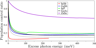
Figure 6: (color online) Calculated population control ratios appropriate for opposite circularly polarized fields normally incident on a $\left(111\right)$ surface of InSb, GaSb, InP, GaAs, and ZnSe. The blue, dotted line is the ratio for linearly polarized fields normally incident on a $\left(111\right)$ surface of GaAs.

The only previous theoretical calculation of the population-control ratio, which was for GaAs, missed finding the large ratio near the band edge because it was based on ab initio calculations of $\xi_{(1)}$, $\xi_{(2)}$ and $\xi_{(I)}$ that had poor spectral resolution near the band edge Fraser et al. (1999). Over the rest of the spectrum shown in Fig. 6, it is about a factor of two smaller than our calculation. This is consistent with the previous calculation being based on a calculation of the two-photon absorption coefficient $\xi_{(2)}$ that is too large by comparison with other calculations Hutchings and Wherrett (1994a); Murayama and Nakayama (1995).

The population-control ratio has been measured only in GaAs Fraser et al. (1999); Fraser and van Driel (2003); Stevens et al. (2003a, 2004a); Stevens et al. (2005). The measured ratios on $\left(111\right)$-GaAs, at excess photon energies of 180 meV Fraser et al. (1999); Fraser and van Driel (2003) and 312 meV Stevens et al. (2003a, 2004a) were 4 to 5 times smaller than our calculation. Some of the difference can be attributed to phase mismatch and large sample thickness Fraser et al. (1999); Fraser and van Driel (2003); Stevens et al. (2003a, 2004a). An experiment on a $\left(110\right)$-grown multiple quantum well was complicated by an additional cascaded second harmonic effect Stevens et al. (2005).

V Spin current

Spin-current density can be quantified by a second-rank pseudotensor $K^{ij}$ defined as the average value of the product $v^{i}S^{j}$, where $\mathbf{v}$ is the velocity operator and $\mathbf{S}$ is the spin operator Bhat and Sipe (2000). Note that some authors alternately choose the first index to represent spin and the second index to represent velocity Rashba (2003). Also, due to the spin-orbit part of the velocity operator—the so-called “anomalous” velocity [the second term in (2)]—$\mathbf{v}$ and $\mathbf{S}$ do not commute, and thus $v^{i}S^{j}$ is not Hermitian. Instead, one should take $(v^{i}S^{j}+S^{j}v^{i})/2$ as the operator for spin-current. But since we neglect the anomalous velocity (see Appendix A), this is not necessary.

The spin-current injection rate due to the field (1) can be written

$$\dot{K}^{ij}=\mu_{\left(1\right)}^{ijkl}E_{2\omega}^{k*}E_{2\omega}^{l}+\dot{K}_{(I)}^{ij}+\mu_{\left(2\right)}^{ijklmn}E_{\omega}^{k*}E_{\omega}^{l*}E_{\omega}^{m}E_{\omega}^{n},$$ (24)

where the pseudotensor $\mu_{\left(1\right)}^{ijkl}$ describes one-photon spin-current injection Bhat et al. (2005a), the pseudotensor $\mu_{\left(2\right)}^{ijklmn}$ describes two-photon spin-current injection, and

$$\dot{K}_{(I)}^{ij}=\mu_{(I)}^{ijklm}E_{\omega}^{*k}E_{\omega}^{*l}E_{2\omega}^{m}+c.c.$$ (25)

is “1+2” spin-current injection Bhat and Sipe (2000). The fifth-rank pseudotensor $\mu_{(I)}^{ijklm}$ has intrinsic symmetry $\mu_{(I)}^{ijlkm}=\mu_{(I)}^{ijklm}$. In an isotropic material, $\mu_{(I)}^{ijklm}$ has three independent components, while in a cubic material (with $T_{d}$, $O$, or $O_{h}$ symmetry) $\mu_{(I)}^{ijklm}$ has six independent components. The four parameters $A_{i}$, $i=1$–$4$, that we used previously to describe spin-current injection in an isotropic model Bhat and Sipe (2000) can be reduced to three independent components with identities such as $\varepsilon^{ijm}\delta^{kl}-\varepsilon^{ijk}\delta^{lm}+\varepsilon^{jkm}\delta^{il}-\varepsilon^{ikm}\delta^{jl}=0$ Kearsley and Fong (1975). For a cubic material, $\mu_{(I)}^{ijklm}$ has 54 non-zero elements in the principal cubic basis, and can be written

$$\begin{split}\mu_{(I)}^{ijklm}=&\frac{\mu_{N1}}{2}\left(\varepsilon^{jml}\delta^{ik}+\varepsilon^{jmk}\delta^{il}\right)+\mu_{N3}\varepsilon^{ijm}\delta^{kl}\\ &+\frac{\mu_{N2}}{2}\left(\varepsilon^{iml}\delta^{jk}+\varepsilon^{imk}\delta^{jl}\right)+\mu_{C1}\delta^{ikln}\varepsilon^{njm}\\ &+\mu_{C2}\delta^{jkln}\varepsilon^{nim}+\frac{\mu_{C3}}{2}\left(\delta^{ijkn}\varepsilon^{nml}+\delta^{ijln}\varepsilon^{nmk}\right),\end{split}$$ (26)

where the non-isotropic tensor $\delta^{ijkl}$ has nonzero components $\delta^{aaaa}=\delta^{bbbb}=\delta^{cccc}=1$, where $a$, $b$, and $c$ denote components along the principal cubic axes. The six independent components are $\mu_{N1}\equiv 2\mu_{(I)}^{acaba}$, $\mu_{N2}\equiv 2\mu_{(I)}^{caaba}$, $\mu_{N3}\equiv\mu_{(I)}^{abccc}$, $\mu_{C1}\equiv\mu_{(I)}^{abaac}-\mu_{N1}-\mu_{N3}$, $\mu_{C2}\equiv\mu_{(I)}^{baaac}-\mu_{N2}+\mu_{N3}$, and $\mu_{C3}\equiv 2\mu_{(I)}^{aaacb}-\mu_{N1}-\mu_{N2}$. Thus in a cubic material,

$$\begin{split}\dot{K}_{(I)}^{ij}=&\mu_{N1}E_{\omega}^{*i}\left(\mathbf{E}_{2\omega}\times\mathbf{E}_{\omega}^{*}\right)^{j}+\mu_{N2}\left(\mathbf{E}_{2\omega}\times\mathbf{E}_{\omega}^{*}\right)^{i}E_{\omega}^{*j}\\ &+\mu_{N3}\varepsilon^{ijk}E_{2\omega}^{k}\left(\mathbf{E}_{\omega}^{*}\cdot\mathbf{E}_{\omega}^{*}\right)+\mu_{C3}\delta^{ijkl}E_{\omega}^{*k}\left(\mathbf{E}_{2\omega}\times\mathbf{E}_{\omega}^{*}\right)^{l}\\ &+\left(\mu_{C1}\delta^{ikln}\varepsilon^{njm}+\mu_{C2}\delta^{jkln}\varepsilon^{nim}\right)E_{\omega}^{*k}E_{\omega}^{*l}E_{2\omega}^{m}+c.c.\end{split}$$ (27)

Note that the injection of $\left\langle\mathbf{v\cdot S}\right\rangle$ is zero in a cubic material, i.e., $\dot{K}^{ij}$ is traceless. In an isotropic model, such as the one we used previously Bhat and Sipe (2000), $\mu_{C1}=\mu_{C2}=\mu_{C3}=0$. The connection to our previous notation is $\mu_{N1}=D\left(A_{1}-A_{4}\right)$, $\mu_{N2}=D\left(A_{2}+A_{4}\right)$, and $\mu_{N3}=D\left(A_{3}+A_{4}\right)$ Bhat and Sipe (2000).

The spin-current injection can be divided into a contribution from electrons $\dot{K}^{ij}_{(I;e)}$, and a contribution from holes $\dot{K}^{ij}_{(I;h)}$; that is, $\dot{K}^{ij}_{(I)}=\dot{K}^{ij}_{(I;e)}+\dot{K}^{ij}_{(I;h)}$ (similarly, $\mu^{ijklm}_{(I)}=\mu^{ijklm}_{(I;e)}+\mu^{ijklm}_{(I;h)}$). Expressions in the PBA for both the electron and hole spin current are given elsewhere Bhat and Sipe (2000); here we focus on the electron spin current, since hole spin relaxation is typically very fast Hilton and Tang (2002); Yu et al. (2005).

A microscopic expression for the spin-current injection was derived previously in the Fermi’s golden rule (FGR) limit of perturbation theory and applied to a model in which all bands are doubly degenerate Bhat and Sipe (2000). However, it is unsuitable for a calculation with $H_{14}$, which accounts for the small splitting of the spin degeneracy that occurs in materials of zinc-blende symmetry Dresselhaus (1955); Cardona et al. (1988); Pikus et al. (1988). If the spin-split bands were well separated, then the microscopic expression for $\dot{K}^{ij}_{(I;e)}$ would be

$$\begin{split}\dot{K}^{ij}_{(I;e)}=&\frac{2\pi}{L^{3}}\sum_{c,v,\mathbf{k}}\left\langle c\mathbf{k}\right|v^{i}S^{j}\left|c\mathbf{k}\right\rangle\\ &\times\left[\left(\Omega_{c,v,\mathbf{k}}^{\left(2\right)}\right)^{*}\Omega_{c,v,\mathbf{k}}^{\left(1\right)}+c.c.\right]\delta\left(2\omega-\omega_{cv}\left(\mathbf{k}\right)\right),\end{split}$$

where $L^{3}$ is a normalization volume; the one-photon amplitude $\Omega_{c,v,\mathbf{k}}^{\left(1\right)}$ is

$$\Omega_{c,v,{\mathbf{k}}}^{\left(1\right)}=i\frac{e}{2\hbar\omega}\mathbf{E}_{2\omega}\cdot\mathbf{v}_{c,v}\left(\mathbf{k}\right),$$ (28)

where the charge on an electron is $e$ ($e<0$), and the two-photon amplitude $\Omega_{c,v,\mathbf{k}}^{\left(2\right)}$ is

$$\Omega_{c,v,\mathbf{k}}^{(2)}=\left(\frac{e}{\hbar\omega}\right)^{2}\sum_{n}\frac{\left(\mathbf{E}_{\omega}\cdot\mathbf{v}_{c,n}\left(\mathbf{k}\right)\right)\left(\mathbf{E}_{\omega}\cdot\mathbf{v}_{n,v}\left(\mathbf{k}\right)\right)}{\omega_{nv}\left(\mathbf{k}\right)-\omega}.$$ (29)

However, for the photon energies and materials studied here, the spin-splitting is small; it is comparable to the broadening that one would calculate from the scattering time of the states, and also to the laser bandwidth for typical ultrafast experiments. Thus, the spin-split bands should be treated as quasidegenerate in FGR, with the result

$$\begin{split}\dot{K}_{(I;e)}^{ij}=&\frac{2\pi}{L^{3}}\sum_{c,c^{\prime}}^{\prime}\sum_{v,\mathbf{k}}\langle c\mathbf{k}|v^{i}S^{j}|c^{\prime}\mathbf{k}\rangle\left(\Omega_{c,v,\mathbf{k}}^{\left(2\right)}\right)^{*}\Omega_{c^{\prime},v,\mathbf{k}}^{\left(1\right)}\\ &\times\frac{1}{2}\left[\delta\left(2\omega-\omega_{cv}\left(\mathbf{k}\right)\right)+\delta\left(2\omega-\omega_{c^{\prime}v}\left(\mathbf{k}\right)\right)\right]+c.c.,\end{split}$$

where the prime on the summation indicates a restriction to pairs $\left(c,c^{\prime}\right)$ for which either $c^{\prime}=c$, or $c$ and $c^{\prime}$ are a quasidegenerate pair. The optical excitation of the coherence between spin-split bands can be justified using the semiconductor optical Bloch equation approach, as was done for the one-photon spin properties Bhat et al. (2005a). Note that this issue does not arise for “1+2” current injection or “1+2” population control, since $\langle c\mathbf{k}|\mathbf{v}|c^{\prime}\mathbf{k}\rangle$ and $\langle c\mathbf{k}|c^{\prime}\mathbf{k}\rangle$ vanish between spin-split bands.

Using the time-reversal properties of the Bloch functions, we find that $\mu_{(I;e)}$ is real, and can be written as

$$\begin{split}\mu_{(I;e)}^{ijklm}=&i\left(\frac{e}{\hbar\omega}\right)^{3}\frac{\pi}{2L^{3}}\sum_{c,c^{\prime}}^{\prime}\sum_{v,\mathbf{k}}\sum_{n}\delta\left(2\omega-\omega_{cv}\left(\mathbf{k}\right)\right)\\ &\times\mathrm{Re}\left\{\frac{\left\langle c\mathbf{k}\right|v^{i}S^{j}\left|c^{\prime}\mathbf{k}\right\rangle}{\omega_{nv\mathbf{k}}-\omega}\left[M_{c,c^{\prime},v}^{klm}-\left(M_{c^{\prime},c,v}^{klm}\right)^{*}\right]\right\},\end{split}$$ (30)

where

$$M_{c,c^{\prime},v}^{klm}\equiv\frac{1}{2}v_{c^{\prime}v}^{m}(\mathbf{k})\left[v_{cn}^{k*}(\mathbf{k})v_{nv}^{l*}(\mathbf{k})+v_{cn}^{l*}(\mathbf{k})v_{nv}^{k*}(\mathbf{k})\right].$$ (31)

That $\mu_{(I;e)}$ in (30) is purely real is a consequence of the independent-particle approximation Bhat and Sipe (2005).

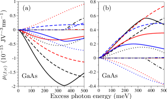
Figure 7: (color online): Calculated spectra of GaAs spin-current injection components and their contributions from each initial valence band; dashed, dotted, and dashed-dotted lines include only transitions from the $hh$, $lh$, and $so$ bands respectively, while the solid lines include all three transitions. Panel (a) shows $\mu_{N1}$ (black lines), $\mu_{N2}$ (red lines), and $\mu_{N3}$ (blue lines). Panel (b) shows $\mu_{C1}$ (black lines), $\mu_{C2}$ (red lines), and $\mu_{C3}$ (blue lines).

V.1 Calculation results

The spectra of the independent components of $\mu_{(I;e)}$, calculated for GaAs, are shown in Fig. 7 and Fig. 8. Figure 7 also shows contributions from each possible initial valence band. Figure 8 shows the spin-current injection calculated with various degrees of approximation described in Sec. II.4. The only other calculation of “1+2” spin-current injection for bulk GaAs is our earlier calculation, which used a spherical, parabolic-band approximation to the eight-band model and did not include the $so$ band as an intermediate state Bhat and Sipe (2000); it is shown in Fig. 8 for $\mu_{N1}$, $\mu_{N2}$, and $\mu_{N3}$.

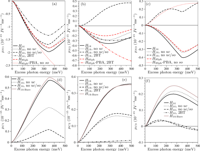
Figure 8: (color online): Approximations for GaAs spin current components (a) $\mu_{N1}$, (b) $\mu_{N2}$, (c) $\mu_{N3}$, (d) $\mu_{C1}$, (e) $\mu_{C2}$, (f) $\mu_{C3}$. The approximations are described in Sec. II.4.

The term $\mu_{N1}$ has the largest magnitude of the six independent parameters of $\mu_{(I;e)}$. Since it is negative for $hh$ and $lh$ transitions but positive for $so$ transitions, it peaks in magnitude at $2\hbar\omega$ just above $E_{g}+\Delta_{0}$ (the energy at which $so$ transitions become allowed). Two band terms make the largest contribution to $\mu_{N1}$, followed by three-band terms with $hh$ or $lh$ intermediate states. The $so$ and $uc$ intermediate states make a very small contribution to $\mu_{N1}$ for excess energies less than 200 meV. The warping of the bands is not important for $\mu_{N1}$, since the calculation with $H_{8\text{Sph}}$ closely approximates the “$H_{14}$, no $uc$” calculation, which includes the same intermediate states. The “$H_{8\text{Sph}}$-PBA, no $so$” calculation, which we derived previously Bhat and Sipe (2000), is a good approximation to $\mu_{N1}$ at excess energies below 250 meV; nonparabolicity becomes important at higher energies. The $hh$ contribution has a larger magnitude than the $lh$ contribution in part because three-band terms increase the magnitude of the $hh$ contribution, but decrease that of the $lh$ contribution, as expected from the PBA expression (42a).

The term $\mu_{N2}$ is negative for $hh$ transitions, positive for $lh$ transitions, and negligible for $so$ transitions. The calculation “$H_{14}$, 2BT” is a good approximation to the calculation $H_{14}$. However, the three-band terms are not small; rather, they nearly cancel. In particular the transition $hh$-$lh$-$c$ makes a large positive contribution to $\mu_{N2}$, while the transition $hh$-$so$-$c$ makes a large negative contribution. Since our earlier PBA calculation included the former but not the latter Bhat and Sipe (2000), it is a poor approximation to $\mu_{N2}$. But by including only 2BTs, it is a fair approximation for excess energies less than 200 meV. This agreement is fortuitous, since the calculation $H_{8\text{Sph}}$ underestimates the magnitude of $\mu_{N2}$, and the PBA leads to an overestimation of the magnitude of $\mu_{N2}$.

The term $\mu_{N3}$ is negligible when only 2BTs are included, in agreement with the PBA Bhat and Sipe (2000). The $hh$-$lh$-$c$ transitions are positive, while the $lh$-$hh$-$c$ transitions are negative; the former is larger, and thus $\mu_{N3}$ is positive when $so$ intermediate states are neglected. Both $lh$-$so$-$c$ and $hh$-$so$-$c$ are negative and substantial enough to make the total $\mu_{N3}$ negative. Consequently, our earlier PBA result Bhat and Sipe (2000), which neglects $so$ intermediate states, is a poor approximation to $\mu_{N3}$. Upper conduction bands make a fairly small contribution to $\mu_{N3}$, and warping does not seem to be important for $\mu_{N3}$ since the calculation with $H_{8\text{Sph}}$ is a good approximation.

As expected, the terms $\mu_{C1}$, $\mu_{C2}$, and $\mu_{C3}$ are zero when calculated with $H_{8\text{Sph}}$.

The term $\mu_{C1}$ is negligible when only 2BTs are included. Transitions with intermediate states in the set $\left\{hh,lh,so\right\}$ comprise roughly two-thirds of $\mu_{C1}$. The anisotropy of these transitions is not simply due to the warping of the $hh$ and $lh$ bands, which we have determined by a calculation (not shown) using $H_{8}$ without the remote band contribution to the velocity. Rather, it comes from wave function mixing of the $\Gamma_{8c}$ and $\Gamma_{7c}$ states into the valence and $c$ band states. The cubic anisotropy of two-photon absorption has been attributed to such wave function mixing Dvorak et al. (1994); Hutchings and Wherrett (1994a). The other third of the full $\mu_{C1}$ is due to transitions with the $uc$ intermediate state, which would be forbidden close to the $\Gamma$ point if the material were isotropic. We also note that each three-band term makes a positive contribution to $\mu_{C1}$.

The term $\mu_{C2}$ is nearly negligible when only 2BTs are included. Transitions from the $hh$ and $lh$ bands have opposite sign, and those from the $so$ band are negligible. About half of $\mu_{C2}$ is due to the transitions $hh$-$lh$-$c$ and $lh$-$hh$-$c$, and the other half is due to transitions with the $uc$ intermediate states. Transitions with $so$ intermediate states are negligible. As with $\mu_{C1}$, the anisotropy of the $hh$-$lh$-$c$ and $lh$-$hh$-$c$ transitions is due to the wave function mixing of the $\Gamma_{8c}$ and $\Gamma_{7c}$ states into the $hh$, $lh$, and $c$ band states.

The term $\mu_{C3}$ is positive for $hh$ transitions, negative for $lh$ transitions, and negligible for $so$ transitions. The transitions $hh$-$so$-$c$ and $lh$-$so$-$c$ account for most of the value of $\mu_{C3}$, but 2BTs are not negligible. Transitions with $uc$ intermediate states reduce the value of $\mu_{C3}$ by as much as 10%. Most of $\mu_{C3}$, especially at energies less than 200 meV, is due to the warping of the $hh$ and $lh$ bands. Consistent with this, we find that remote band effects are somewhat important for $\mu_{C3}$; when remote band effects are removed, the calculation of $\mu_{C3}$ is about 25% larger than the full calculation. Note that $\mu_{C3}$ is far more sensitive to remote band effects than any other optical property calculated in this article.

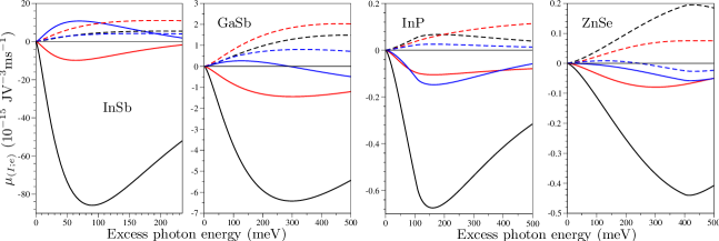
Figure 9: Spectra of spin current components for InSb, GaSb, InP, and ZnSe: $\mu_{N1}$ (solid black line), $\mu_{N2}$ (solid red line), $\mu_{N3}$ (solid blue line), $\mu_{C1}$ (dashed black line), $\mu_{C2}$ (dashed red line), and $\mu_{C3}$ (dashed blue line).

In Fig. 9 we plot the spectra of the independent components of the spin current density pseudotensor for InSb, GaSb, InP, and ZnSe. The spin current tensor is largest for InSb in agreement with the PBA expressions in Appendix B. We also note that $\mu_{N3}$ is positive for InSb and GaSb at low excess photon energy, whereas it is negative for InP, GaAs, and ZnSe.

V.2 Configurations

Co-circularly polarized fields generate a spin-polarized current, which can be characterized by its degree of spin polarization $f\equiv\left(2e/\hbar\right)\dot{K_{e}^{ij}}\hat{q}^{i}\hat{n}^{j}/|\dot{\mathbf{J}_{e}}|$, where $\hat{\mathbf{n}}$ is a unit vector normal to the polarization plane of the fields, and $\hat{\mathbf{q}}$ is a unit vector in the direction of $\mathbf{J}_{e}$ Bhat and Sipe (2000). Essentially, $f=\left\langle vS\right\rangle/\left\langle v\right\rangle$. Since this measure aims to characterize the photoexcited distribution of electrons, we neglect holes from both $\dot{K}$ and $\dot{J}$ in this calculation foo (c). For fields normally incident on a $\left(001\right)$ surface (i.e. $\mathbf{e}_{\omega}=\mathbf{e}_{2\omega}=\left(\mathbf{\hat{x}}\pm i\mathbf{\hat{y}}\right)/\sqrt{2}$), the spin current is

$$\begin{split}\dot{K}_{(I)}^{ij}=&\mp\sqrt{2}|E_{2\omega}||E_{\omega}|^{2}\\ &\times\left[\left(\mu_{N1}+\frac{\mu_{C1}}{2}\right)\hat{m}_{\pm}^{i}\hat{z}^{j}+\left(\mu_{N2}+\frac{\mu_{C2}}{2}\right)\hat{z}^{i}\hat{m}_{\pm}^{j}\right],\end{split}$$

where $\mathbf{\hat{m}}_{\pm}=\sin\left(2\phi_{\omega}-\phi_{2\omega}\right)\mathbf{\hat{x}}\pm\cos\left(2\phi_{\omega}-\phi_{2\omega}\right)\mathbf{\hat{y}}$, the current is $\dot{\mathbf{J}}_{(I)}=\sqrt{2}E_{2\omega}E_{\omega}^{2}\left(\eta_{B1}+\eta_{C}/2\right)\hat{\mathbf{m}}_{\pm}$, and the degree of spin polarization is

$$f=\frac{2e}{\hbar}\frac{\mu_{N1}+\mu_{C1}/2}{\eta_{B1}+\eta_{C}/2}.$$ (32)

For fields normally incident on a $\left(111\right)$ surface, $\dot{\mathbf{J}}_{(I)}=\sqrt{2}E_{2\omega}E_{\omega}^{2}\left(\eta_{B1}+\eta_{C}/3\right)\hat{\mathbf{m}}_{\pm}$, and

$$f=\frac{2e}{\hbar}\frac{\mu_{N1}+\mu_{C1}/3+\mu_{C3}/3}{\eta_{B1}+\eta_{C}/3}.$$ (33)

The degree of spin polarization is plotted for GaAs in Fig. 10(a). The cubic anisotropy is small, but clearly seen, especially at low excess photon energies. The other materials have very similar degrees of spin polarization.

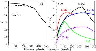
Figure 10: (a) Degree of polarization of spin-polarized current due to co-circularly polarized fields. (b) Displacement of spins in pure spin current due to cross-linearly polarized fields.

A pure spin current, without an electrical current, can be generated with cross-linearly polarized fields Bhat and Sipe (2000). We consider fields polarized in the $\left(001\right)$ plane, with the $\omega$ field polarized at an angle $\theta$ to the $\mathbf{\hat{x}}$ axis (i.e. $\left[100\right]$) and the $2\omega$ field polarized at an angle $\theta$ to the $\mathbf{\hat{y}}$ axis ($\mathbf{e}_{\omega}=\mathbf{\hat{x}}\cos\theta+\mathbf{\hat{y}}\sin\theta$ and $\mathbf{e}_{2\omega}=-\mathbf{\hat{x}}\sin\theta+\mathbf{\hat{y}}\cos\theta$). The spin current is

$$\begin{split}\dot{K}_{(I)}^{ij}=&-\frac{1}{2}|E_{2\omega}||E_{\omega}|^{2}\cos\left(2\phi_{\omega}-\phi_{2\omega}\right)\left[\left(4\mu_{N1}+4\mu_{N3}+3\mu_{C1}+\mu_{C1}\cos\left(4\theta\right)\right)e_{\omega}^{i}\hat{z}^{j}\right.\\ &\left.-\sin\left(4\theta\right)\left(\mu_{C1}e_{2\omega}^{i}\hat{z}^{j}+\mu_{C2}\hat{z}^{i}e_{2\omega}^{j}\right)+\left(4\mu_{N2}-4\mu_{N3}+3\mu_{C2}+\mu_{C2}\cos\left(4\theta\right)\right)\hat{z}^{i}e_{\omega}^{j}\right]\end{split}$$

This pure spin current is typically measured by the resulting displacement of up and down spins Stevens et al. (2003b); Hübner et al. (2003). The finite displacement results from transport and scattering of the electrons. Using the Boltzmann transport equation in the relaxation time approximation with space-charge effects justifiably neglected Hübner et al. (2003), one finds $d^{i}\left(\mathbf{\hat{z}}\right)=\left(4\tau/\hbar\right)\dot{K}^{ij}\hat{z}^{j}/\left(\dot{N}_{\left(1\right)}+\dot{N}_{\left(2\right)}\right)$ Bhat et al. (2005a). Here, $\mathbf{d}\left(\mathbf{\hat{z}}\right)$ is the displacement of spins measured with respect to the quantization direction $\mathbf{\hat{z}}$, and $\tau$ is the momentum relaxation time. We assume the field intensities have been chosen to balance one- and two-photon absorption, a condition that is $\theta$-dependent due to the cubic anisotropy of two-photon absorption. Thus,

$$\mathbf{d}\left(\mathbf{\hat{z}}\right)\cdot\mathbf{e}_{\omega}=\frac{\tau}{\hbar}\frac{\left(4\mu_{N1}+4\mu_{N3}+3\mu_{C1}+\mu_{C1}\cos\left(4\theta\right)\right)}{\sqrt{\xi_{(1)}^{xx}\xi_{(2)}^{xxxx}\left(1-\left(\sigma/2\right)\sin^{2}\left(2\theta\right)\right)}}$$ (34)

and

$$\mathbf{d}\left(\mathbf{\hat{z}}\right)\cdot\mathbf{e}_{2\omega}=\frac{\tau}{\hbar}\frac{\mu_{C1}\sin\left(4\theta\right)}{\sqrt{\xi_{(1)}^{xx}\xi_{(2)}^{xxxx}\left(1-\left(\sigma/2\right)\sin^{2}\left(2\theta\right)\right)}},$$ (35)

where $\sigma$ is the two-photon absorption cubic-anisotropy factor given explicitly in the next section Dvorak et al. (1994); Hutchings and Wherrett (1994a). At $\theta=0$ and $\theta=\pi/4$, $\mathbf{d}$ is parallel to $\mathbf{e}_{\omega}$. The spin separation distance is plotted in Fig. 10(b), where we have assumed a momentum relaxation time of 100 fs for each material.

This calculation of the spin separation distance is a significant improvement over our initial calculations Stevens et al. (2003b); Hübner et al. (2003), which used the eight-band PBA and neglected three-band terms from the two-photon amplitude (“$H_{8\text{Sph}}$-PBA, 2BT”). Stevens et al. measured a spin separation distance of 20 nm in a GaAs multiple quantum well at an excess photon energy of 200 meV, and estimated a momentum relaxation time of $\tau=45$ fs Stevens et al. (2003b). For $\tau=45$ fs, we calculate a spin separation distance of 20.0 nm for bulk GaAs at 200 meV. Hübner et al. measured a spin separation distance of 24 nm (the photoluminescence spot separation is half this distance) in cubic ZnSe at an excess photon energy of 280 meV, and estimated a momentum relaxation time of $\tau=100$ fs Hübner et al. (2003). The calculation in Fig. 10(b) yields $d=23.6$ nm for ZnSe at 280 meV. In both cases, we now find very good agreement with the experiment, whereas the previous model resulted in larger spin separation distances. Of course, this agreement is contingent on the accuracy of the momentum relaxation time estimates.

Note that both the degree of spin polarization for co-circularly polarized fields and the spin-separation distance, plotted in Fig. 10, have a kink at excess photon energy $\Delta_{0}$ and decrease at higher excess photon energies. A similar kink and decrease, due to the onset of transitions from the split-off band, occurs for both one-photon spin injection Dyakonov and Perel (1984) and two-photon spin injection Bhat et al. (2005b).

VI Spin control

The spin injection rate due to the field (1) can be written $\dot{\mathbf{S}}=\dot{\mathbf{S}}_{(1)}+\dot{\mathbf{S}}_{(I)}+\dot{\mathbf{S}}_{(2)}$, where $\mathbf{S}$ is the macroscopic spin density, $\dot{S}_{(1)}^{i}=\zeta_{\left(1\right)}^{ijk}E_{2\omega}^{j*}E_{2\omega}^{k}$ is one-photon spin injection Dyakonov and Perel (1984), $\dot{S}_{(2)}^{i}=\zeta_{(2)}^{ijklm}E_{\omega}^{j*}E_{\omega}^{k*}E_{\omega}^{l}E_{\omega}^{m}$ is two-photon spin injection Bhat et al. (2005b), and

$$\dot{S}_{(I)}^{i}=\zeta_{(I)}^{ijkl}E_{\omega}^{*j}E_{\omega}^{*k}E_{2\omega}^{l}+c.c.$$ (36)

is “1+2” spin control Stevens et al. (2003a). In previous sections and in some of the expressions below, we use $\mathbf{S}$ to denote the single-particle spin operator. It should be obvious by context when $\mathbf{S}$ refers to the macroscopic spin density and when it refers to that spin operator.

The fourth-rank pseudotensor $\zeta_{(I)}^{ijkl}$ has intrinsic symmetry on the indices $j\leftrightarrow k$. Such a pseudotensor is zero in the presence of inversion symmetry; hence, “1+2” spin control requires materials of lower symmetry. For zinc-blende symmetry (point group $T_{d}$), a general fourth-rank pseudotensor has three independent parameters and 18 non-zero elements in the standard cubic basis; forcing the $j\leftrightarrow k$ symmetry leaves two independent parameters

$$i\zeta_{IA} \equiv\zeta_{(I)}^{abba}=\zeta_{(I)}^{caac}=\zeta_{(I)}^{bccb}=-\zeta_{(I)}^{acca}=-\zeta_{(I)}^{cbbc}=-\zeta_{(I)}^{baab},$$ (37a)

$$\begin{split}i\zeta_{IB}&\equiv\zeta_{(I)}^{aabb}=\zeta_{(I)}^{ccaa}=\zeta_{(I)}^{bbcc}=-\zeta_{(I)}^{aacc}=-\zeta_{(I)}^{ccbb}=-\zeta_{(I)}^{bbaa}\\ &=\zeta_{(I)}^{abab}=\zeta_{(I)}^{caca}=\zeta_{(I)}^{bcbc}=-\zeta_{(I)}^{acac}=-\zeta_{(I)}^{cbcb}=-\zeta_{(I)}^{baba}.\end{split}$$ (37b)

The spin injection has a contribution from electrons $\mathbf{\dot{S}}_{(I;e)}$, and a contribution from holes $\mathbf{\dot{S}}_{(I;h)}$; that is, $\mathbf{\dot{S}}_{(I)}=\mathbf{\dot{S}}_{(I;e)}+\mathbf{\dot{S}}_{(I;h)}$, and $\zeta_{(I)}=\zeta_{(I;e)}+\zeta_{(I;h)}$.

We treat the spin-split bands as quasidegenerate when taking the FGR limit of perturbation theory, as discussed for the spin current in Section V, deriving the microscopic expression

$$\begin{split}\mathbf{\dot{S}}_{(I;e)}=&\frac{2\pi}{L^{3}}\sum_{c,c^{\prime}}^{\prime}\sum_{v,\mathbf{k}}\left\langle c\mathbf{k}\right|\mathbf{S}\left|c^{\prime}\mathbf{k}\right\rangle\left(\Omega_{c,v,\mathbf{k}}^{\left(2\right)}\right)^{*}\Omega_{c^{\prime},v,\mathbf{k}}^{\left(1\right)}\\ &\times\frac{1}{2}\left[\delta\left(2\omega-\omega_{cv}\left(\mathbf{k}\right)\right)+\delta\left(2\omega-\omega_{c^{\prime}v}\left(\mathbf{k}\right)\right)\right]+c.c.,\end{split}$$

where the prime on the summation indicates a restriction to pairs $\left(c,c^{\prime}\right)$ for which either $c^{\prime}=c$, or $c$ and $c^{\prime}$ are a quasidegenerate pair. Using the time-reversal properties of the Bloch functions, we find that $\zeta_{(I;e)}$ is purely imaginary and can be written

$$\begin{split}\zeta_{(I;e)}^{ijkl}=&i\left(\frac{e}{\hbar\omega}\right)^{3}\frac{\pi}{2L^{3}}\sum_{c,c^{\prime}}^{\prime}\sum_{v,\mathbf{k}}\sum_{n}\delta\left(2\omega-\omega_{cv}\left(\mathbf{k}\right)\right)\\ &\times\mathrm{Re}\left\{\frac{\left\langle c\mathbf{k}\right|S^{i}\left|c^{\prime}\mathbf{k}\right\rangle}{\omega_{nv\mathbf{k}}-\omega}\left[M_{c,c^{\prime},v}^{jkl}+\left(M_{c^{\prime},c,v}^{jkl}\right)^{*}\right]\right\},\end{split}$$ (38)

where $M_{c,c^{\prime},v}^{jkl}$ is given in Eq. (31).

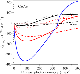
Figure 11: (color online) Spin control pseudotensor components $\zeta_{IA}$ (black lines), $\zeta_{IB}$ (red lines), and $\left(\zeta_{IA}+2\zeta_{IB}\right)$ (blue line) with breakdown into initial states. Dotted lines include transitions from the $lh$ band, dashed lines include transitions from the $hh$ band, dashed-dotted lines include transitions from the $so$ band, and solid lines include all transitions.

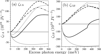
Figure 12: Spin control pseudotensor for GaAs. The calculations are $H_{14}$ (solid black lines), “$H_{14}$, no $uc$” (dotted lines), “$H_{14}$, no $uc$/$so$” (dashed-dotted lines), “$H_{14}$, 2BT” (dashed lines), and “$H_{14}$-PBA” (solid grey lines).

The spectra of $\zeta_{IA}$ and $\zeta_{IB}$ for GaAs are shown in Figs. 11 and 12. Figure 11 also shows the contributions from each possible initial valence band. Figure 12 shows the spin control calculated with various degrees of approximation described in Sec. II.4.

The term $\zeta_{IA}$ decreases from zero at the band edge to a maximum negative value at 40 meV, mostly due to transitions from the $hh$ band, and is positive at higher excess photon energies, mostly due to transitions from the $lh$ band. The low energy behavior is in agreement with the PBA result (43a), in which the ratio of $hh:lh$ transitions is $\left(m_{c,hh}/m_{c,lh}\right)^{3/2}$. Transitions with $so$ and $uc$ intermediate states dominate the decrease in $\zeta_{IA}$ at low excess photon energies, as seen in Fig. 12(a); they are the only non-zero transitions in the PBA result (43a). The contribution from $uc$ intermediate states is negative and approximately constant over most of the spectrum, whereas the contribution from $so$ intermediate states changes from negative to positive as transitions from the $so$ band become allowed ($2\hbar\omega>E_{g}+\Delta_{0}$). The contribution from 2BTs, which is zero in the PBA, is positive over the whole spectrum. The breakdown of the PBA is due to the increase in magnitude of the 2BTs. In fact, the sum of the PBA and the 2BTs is a good approximation to the full calculation. We also note that a calculation with $H_{8}$ for $\zeta_{IA}$ yields a nearly negligible result; thus, the contribution from intermediate states within the set $\left\{so,lh,hh,c\right\}$ (including 2BTs) is due to the mixing of the $\Gamma_{7c}$ and $\Gamma_{8c}$ wavefunctions with these states.

The term $\zeta_{IB}$ is larger in magnitude than the term $\zeta_{IA}$ over most of the calculated spectrum. It falls to a maximum negative value at 95 meV, sharply increases when transitions from the $so$ band become allowed, and is positive at higher excess photon energy. At lower photon energies, transitions from the $hh$ band and transitions from the $lh$ band both make negative contributions to $\zeta_{IB}$; in the PBA result (43b) the ratio of $hh:lh$ transitions is $\left(m_{c,hh}/m_{c,lh}\right)^{3/2}$. Fig. 12(b) reveals that $\zeta_{IB}$ is essentially due to contributions from $uc$ intermediate states, and 2BTs. Over the whole spectrum, the former are negative while the latter are positive. The smallness of the contribution from $so$ intermediate states is also seen in the PBA result (43b), since $Z_{+}\gg Z_{-}^{\prime}$ in that expression. We also note that a calculation with $H_{8}$ for $\zeta_{IB}$ yields a nearly negligible; thus, the contribution from intermediate states within the set $\left\{so,lh,hh,c\right\}$ (including 2BTs) is due to the mixing of the $\Gamma_{7c}$ and $\Gamma_{8c}$ wave functions with these states.

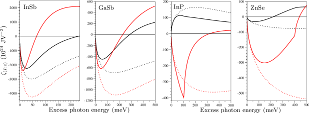
Figure 13: (color online) Spin control calculated for InSb, GaSb, InP, and ZnSe. Black lines are $\zeta_{IA}$ and red lines are $\zeta_{IB}$. Solid lines are the full calculation using $H_{14}$. Dotted lines are the parabolic-band approximation calculated with (43a) and (43b).

We have also calculated the spin-control pseudotensor for the semiconductors InSb, GaSb, InP, and ZnSe. The results are shown in Fig. 13 along with the parabolic-band approximations (43a) and (43b).

The magnitude of spin control is determined by $\zeta_{(I)}$, but in an experiment one is more interested in the depth of the phase-dependent modulation of the spin polarization signal. One possible definition for the signal is the ratio of spin injection measured with both $\omega$ and $2\omega$ fields to the sum of the spin injections measured with circularly polarized fields of each frequency Stevens et al. (2003a). The amplitude of its modulation is

$$\frac{\left|\dot{S}_{(I)}^{z}\right|}{\dot{S}_{(1)}^{z}\left(\sigma^{+}\right)+\dot{S}_{(2)}^{z}\left(\sigma^{+}\right)},$$ (39)

where the argument $\left(\sigma^{+}\right)$ indicates injection with a $\sigma^{+}$ polarized field. This ratio, which is largest for field amplitudes that equalize $\dot{S}_{(1)}^{z}\left(\sigma^{+}\right)$ and $\dot{S}_{(2)}^{z}\left(\sigma^{+}\right)$, was measured by Stevens et al. with excess photon energies of 150 meV and 280 meV Stevens et al. (2003a); Stevens et al. (2005).

The ratio (39) has an undesirable feature: it can exceed unity. Close to the band edge in many semiconductors (at 2 meV in GaAs), there is a photon energy for which $\dot{S}_{(2)}^{z}\left(\sigma^{+}\right)=0$ Bhat et al. (2005b). At that photon energy, it is impossible to choose field amplitudes to balance one- and two-photon spin injection with circular polarized fields [$\dot{S}_{(1)}^{z}\left(\sigma^{+}\right)=\dot{S}_{(2)}^{z}\left(\sigma^{+}\right)$], and thus the maximum ratio has a singularity. Even if the condition $\dot{S}_{(1)}\left(\sigma^{+}\right)=\dot{S}_{(2)}\left(\sigma^{+}\right)$ is relaxed, the ratio (39) can exceed unity. This is because $\dot{S}_{(1)}^{z}\left(\sigma^{+}\right)$ and $\dot{S}_{(2)}^{z}\left(\sigma^{+}\right)$ have opposite sign close to the band gap Bhat et al. (2005b), and thus it is possible, by appropriate choice of field amplitudes, to make the denominator of the ratio arbitrarily small.

An alternate ratio to characterize the spin control, which has an upper bound of unity, is

$$R_{S}=\frac{2}{\hbar}\frac{\left|\dot{S}_{(I)}^{z}\right|}{\dot{N}_{(1)}+\dot{N}_{(2)}}.$$ (40)

It is the amplitude of phase-dependent oscillation of the degree of spin polarization, and it is most useful when there is little or no population control. We assume the fields are chosen to balance one- and two-photon absorption. For most photon energies and materials this is nearly the same as balancing one- and two-photon spin injection.

For normal incidence on a $\left(111\right)$ sample, opposite circularly polarized fields yield

$$R_{S}=\frac{2}{\hbar}\frac{\left|\zeta_{IA}+2\zeta_{IB}\right|}{\sqrt{3\xi_{(1)}^{aa}\xi_{(2)}^{aaaa}\left(1-\sigma/6-\delta\right)}}.$$

For normal incidence on a $\left(110\right)$ sample, opposite circularly polarized fields

$$R_{S}=\frac{2}{\hbar}\frac{3\left|\zeta_{IA}+2\zeta_{IB}\right|}{4\sqrt{2\xi_{(1)}^{aa}\xi_{(2)}^{aaaa}\left(1-\delta-\sigma/8\right)}},$$

and orthogonal linearly polarized fields ($xy$-polarized) yield

$$R_{S}\left(\alpha\right)=\frac{2}{\hbar}\frac{\left|\left(\zeta_{IA}+2\zeta_{IB}\right)\left(r+3\sin^{2}\alpha\right)\cos\alpha\right|}{2\sqrt{\xi_{(1)}^{aa}\xi_{(2)}^{aaaa}\left(1-\frac{1}{2}\sigma\left(\sin^{2}\alpha\right)\left(1+3\cos^{2}\alpha\right)\right)}},$$

where $r\equiv-2\zeta_{IA}/(\zeta_{IA}+2\zeta_{IB})$ Stevens et al. (2003a), and $\alpha$ is the angle between the polarization of the $\omega$ field ($\mathbf{E}_{\omega}$) and the $\left[001\right]$ axis, which lies in the $\left(110\right)$ plane. The angle that maximizes $R_{S}$ depends on photon energy through $r$ and $\sigma$. We determine it numerically.

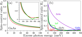
Figure 14: (color online) Spin-control ratio normalized by carrier population [Eq. (40)]. In (a), for GaAs, black lines are $\left(111\right)$-incident, opposite circularly polarized fields; green lines are $\left(110\right)$-incident, opposite circularly polarized fields; and red lines are $\left(110\right)$-incident, orthogonal linearly polarized fields. In (b), for InSb, GaSb, InP, GaAs, and ZnSe, solid lines are $\left(111\right)$-incident, opposite circularly polarized fields. The dotted line in (b) is $\left(110\right)$-incident, orthogonal linearly polarized fields for InP.

The ratio $R_{S}$ for GaAs is plotted in Fig. 14(a). For $\left(111\right)$-incidence, opposite circularly polarized fields yield the highest ratio over the studied range of photon energies. For $\left(110\right)$-incidence, opposite circularly polarized fields yield the highest ratio, except for between 190 meV and 415 meV when $xy$-polarized fields the highest ratio. For $xy$-polarized fields, the angle that yields the largest ratio decreases from 0.99 rad to 0.53 rad from the band edge to 320 meV, and is zero for higher excess energies.

The ratio $R_{S}$ for the five semiconductors InSb, GaSb, InP, GaAs, and ZnSe are plotted in Fig. 14(b). At low photon energy, opposite circularly polarized fields normally incident on $\left(111\right)$ yield the largest ratio for InSb, GaSb, GaAs, and ZnSe, whereas orthogonal linearly polarized fields normally incident on $\left(110\right)$ yield the largest ratio for InP.

VII Summary

We have studied the four “1+2” coherent control effects—current injection, spin-current injection, population control, and spin control—in bulk semiconductors having zinc-blende symmetry. We used an empirical, fourteen-band $\mathbf{k}\cdot\mathbf{p}$ Hamiltonian and examined the relative importance to each effect of the possible initial and intermediate states. We have also studied the crystal orientation and polarization dependencies of each effect. Cubic anisotropy is small in some cases, but large in others.

We have compared the numerical calculation with analytic expressions, derived in the parabolic-band approximation, to show the value and limitations of the latter. The PBA expressions, where they are accurate, are useful to show how the effects scale in different materials.

The comparison between the two approaches establishes that, at low excess photon energies, “1+2” current injection and “1+2” spin-current injection are due to interference of allowed one-photon transitions and allowed-forbidden two-photon transitions, whereas “1+2” population control and “1+2” spin control are due to interference of allowed one-photon transitions and allowed-allowed two photon transitions. It also explains the large population- and spin-control ratios predicted by the fourteen-band calculation close to the band edge, where allowed-allowed two-photon transitions dominate allowed-forbidden two-photon transitions. Neither “1+2” population control, nor “1+2” spin control have yet been experimentally studied in that spectral range.

Appendix A Neglect of the anomalous velocity and $\mathbf{k}$-dependent spin-orbit coupling

The anomalous velocity, i.e. $\mathbf{v}_{A}\equiv\left(\mathbf{v}-\mathbf{p}/m\right)=\hbar\left(\bm{\sigma}\times\bm{\nabla}V\right)/\left(4m^{2}c^{2}\right)$, which leads to $\mathbf{k}$-dependent spin-orbit coupling in $H_{\mathbf{k}}$ from the term $\hbar\mathbf{k}\cdot\mathbf{v}_{A}$, is often neglected in $\mathbf{k}\cdot\mathbf{p}$ models Kane (1956); Cardona and Pollak (1966); Rössler (1984); Pfeffer and Zawadzki (1990, 1996). Some authors have treated matrix elements of $\bm{\nabla}V$ as additional independent parameters Dresselhaus (1955); Rustagi (1969); Bahder (1990); Ostromek (1996). For example, Bahder, who gives the matrix for $\hbar\mathbf{k}\cdot\mathbf{v}_{A}$ within the eight-band model, defines the model parameter Bahder (1990); foo (d)

$$C_{0}\equiv\frac{1}{\sqrt{3}}\frac{\hbar^{2}}{4m^{2}c^{2}}\left\langle S\right|\nabla_{x}V\left|X\right\rangle.$$

Ostromek used the value $C_{0}=0.16$ eV Å to fit the eight-band model to experimental results Ostromek (1996). We here relate matrix elements of $\bm{\nabla}V$ (and hence matrix elements of $\mathbf{v}_{A}$) to other parameters of the model, thereby demonstrating that they can be neglected for the effects we consider.

Bir and Pikus showed that the identity $\left[H_{0},\mathbf{p}\right]=i\hbar\bm{\nabla}V$ leads to $\left\langle X\right|\nabla_{y}V\left|Z\right\rangle=0$ Bir and Pikus (1974). An application of that identity to the remaining nonzero matrix elements yields

$$\left\langle S\right|\nabla_{x}V\left|X\right\rangle =\frac{mP_{0}}{\hbar^{2}}\left(E_{S}-E_{X}\right),$$ (41a)

$$\left\langle S\right|\nabla_{x}V\left|x\right\rangle =-\frac{mP_{0}^{\prime}}{\hbar^{2}}\left(E_{x}-E_{S}\right),$$ (41b)

$$\left\langle X\right|\nabla_{y}V\left|z\right\rangle =\left\langle Z\right|\nabla_{y}V\left|x\right\rangle=-\frac{mQ}{\hbar^{2}}\left(E_{x}-E_{X}\right),$$ (41c)

and similar results for cyclic permutations and Hermitian conjugates of these. The energies $E_{S}$, $E_{X}$, and $E_{x}$ are the eigenvalues of $\left|S\right\rangle$, $\left|X\right\rangle$, and $\left|x\right\rangle$ with respect to the Hamiltonian $H_{0}$. Their values are fixed by the requirement that the eigenvalues of $H_{\mathbf{k}=\mathbf{0}}$ yield the parameters $E_{g}$, $E_{0}^{\prime}$, $\Delta_{0}$, and $\Delta_{0}^{\prime}$ Pfeffer and Zawadzki (1990). Neglecting the small contribution from $\Delta^{-}$, $E_{S}-E_{X}=E_{g}+\Delta_{0}/3$, $E_{x}-E_{S}=E_{0}^{\prime}-E_{g}+2\Delta_{0}^{\prime}/3$, and $E_{x}-E_{X}=E_{0}^{\prime}+2\Delta_{0}^{\prime}/3+\Delta_{0}/3$.

Thus, (41a) gives matrix elements of $\bm{\nabla}V$ in terms of other model parameters. In particular, with parameters from Table 1 for GaAs, we find $C_{0}=5\times 10^{-6}$ eVÅ.

From the point of view of the theory of invariants Suzuki and Hensel (1974); Trebin et al. (1979); Bir and Pikus (1974); Winkler (2003), $\mathbf{k}$-dependent spin-orbit coupling amounts to using different values of $P_{0}$ for $\Gamma_{8}$ and $\Gamma_{7}$ valence bands (and similar changes for $P_{0}^{\prime}$ coupling and $Q$ coupling) Winkler (2003). In terms of $C_{0}$, $P_{0}\rightarrow P_{7}\equiv P_{0}+2\sqrt{3}C_{0}$ for couplings with $\Gamma_{7}$ bands and $P_{0}\rightarrow P_{8}\equiv P_{0}-\sqrt{3}C_{0}$ for couplings with $\Gamma_{8}$ bands. From (41a),

$$\frac{P_{7}-P_{8}}{P_{0}}=\frac{\sqrt{3}C_{0}}{P_{0}}=\frac{3\left(E_{S}-E_{X}\right)}{4mc^{2}}\approx\frac{3E_{g}-\Delta_{0}}{4mc^{2}}.$$

This is very small, since the numerator is on the order of eV, whereas $mc^{2}=5.11\times 10^{5}$ eV. And since this relative change in the matrix element depends on the ratio of $C_{0}$ to $P_{0}$, even the overly large coupling value of $C_{0}=0.16$ eVÅ has only a small effect on optical properties Bhat et al. (2005a, b).

For comparison, consider interband spin-orbit coupling parameterized by $\Delta^{-}$. In the eight-band model, interband spin-orbit coupling is a remote band effect (since it is a coupling with the $uc$ bands), which effectively causes $P_{0}\rightarrow\widetilde{P}_{7}\equiv P_{0}+\left(2\Delta^{-}P_{0}^{\prime}\right)/\left[3\left(E_{0}^{\prime}+\Delta_{0}\right)\right]$ and $P_{0}\rightarrow\widetilde{P}_{8}\equiv P_{0}-\left(\Delta^{-}P_{0}^{\prime}\right)/\left[3\left(E_{0}^{\prime}+\Delta_{0}^{\prime}\right)\right]$. Thus,

$$\frac{\widetilde{P}_{7}-\widetilde{P}_{8}}{P_{0}}\approx\frac{\Delta^{-}}{E_{0}^{\prime}}\frac{P_{0}^{\prime}}{P_{0}}.$$

This effect, which is included in our calculation, is small (it is $4\times 10^{-3}$ in GaAs), but it is orders of magnitude larger than the relative change due to $\mathbf{k}$-dependent spin-orbit coupling.

The above suggests that $\mathbf{k}$-dependent spin-orbit coupling can be neglected for the processes we consider in bulk, cubic materials.

Appendix B Parabolic band approximations

In this appendix, we discuss parabolic-band approximation (PBA) expressions, which are perturbative in the Bloch wave vector $\mathbf{k}$, for “1+2” coherent control effects.

B.1 Current

There have been several different calculations of $\eta$ in the PBA Atanasov et al. (1996); Sheik-Bahae (1999); Bhat and Sipe (2000, 2005). Using a two-band model (one conduction and one valence band), Atanasov et al. obtained $\eta_{B1}\propto\left(2\hbar\omega-E_{g}\right)^{3/2}$ and $\eta_{B2}=0$ Atanasov et al. (1996). Using a three-band model, but only accounting for two-band terms, Shiek-Bahae studied the approximate scaling of “1+2” current injection spectra with the band gap $E_{g}$ and concluded that $\eta_{B1}$ and $\eta_{B2}$ are proportional to $E_{g}^{-2}\left(2x-1\right)^{3/2}\left(2x\right)^{-4}$, where $x\equiv\hbar\omega/E_{g}$ Sheik-Bahae (1999). Our earlier PBA calculation was based on an 8-band model, included both two- and three-band terms in the two-photon amplitude, but did not include terms with the $so$ band as an intermediate state Bhat and Sipe (2000). More recently, we included the $so$ band as an intermediate state, but only for two-band terms Bhat and Sipe (2005). The 2BTs in the 8-band model result differ from the 2BTs in the three-band model result of Sheik-Bahae by material independent factors.

B.2 Spin Current

The spin current PBA result is presented elsewhere Bhat and Sipe (2000). Here we summarize our earlier result in a new notation. For the electron spin current, $\mu_{C1}=\mu_{C2}=\mu_{C3}=0$, and

$$\begin{split}\mu_{N1;e}&=D\frac{m}{m_{c}}\left(\frac{m_{c,hh}}{m}\right)^{3/2}\left(1+Z_{c}\right)-D\frac{m}{m_{c}}\left(\frac{m_{c,hh}}{m}\right)^{5/2}\frac{E_{P}}{3E_{g}}\frac{1-Z_{c}}{1+xm_{c,hh}/m_{hh,lh}}\\ &\quad+D\frac{m}{m_{c}}\left(\frac{m_{c,lh}}{m}\right)^{3/2}\left(\frac{7}{3}-Z_{c}\right)-D\frac{m}{m_{c}}\left(\frac{m_{c,lh}}{m}\right)^{5/2}\frac{E_{P}}{3E_{g}}\frac{1}{1-xm_{c,lh}/m_{hh,lh}},\end{split}$$ (42a)

$$\begin{split}\mu_{N2;e}&=D\frac{m}{m_{c}}\left(\frac{m_{c,hh}}{m}\right)^{3/2}\left(1+Z_{c}\right)-3D\frac{m}{m_{c}}\left(\frac{m_{c,hh}}{m}\right)^{5/2}\frac{E_{P}}{3E_{g}}\frac{1-Z_{c}}{1+xm_{c,hh}/m_{hh,lh}}\\ &\quad-D\frac{m}{m_{c}}\left(\frac{m_{c,lh}}{m}\right)^{3/2}\left(1-\frac{7}{3}Z_{c}\right)-Z_{c}D\frac{m}{m_{c}}\left(\frac{m_{c,lh}}{m}\right)^{5/2}\frac{E_{P}}{3E_{g}}\frac{1}{1-xm_{c,lh}/m_{hh,lh}},\end{split}$$ (42b)

$$\begin{split}\mu_{N3;e}&=-2D\frac{m}{m_{c}}\left(\frac{m_{c,hh}}{m}\right)^{5/2}\frac{E_{P}}{3E_{g}}\frac{1-Z_{c}}{1+xm_{c,hh}/m_{hh,lh}}\\ &\quad+2\left(1-Z_{c}\right)D\frac{m}{m_{c}}\left(\frac{m_{c,lh}}{m}\right)^{5/2}\frac{E_{P}}{3E_{g}}\frac{1}{1-xm_{c,lh}/m_{hh,lh}},\end{split}$$ (42c)

where $x\equiv\left(2\hbar\omega-E_{g}\right)/\left(\hbar\omega\right)$, $m_{n,m}^{-1}=m_{n}^{-1}-m_{m}^{-1}$, $D$ is given in Ref. Bhat and Sipe, 2000, and $Z_{c}\equiv\frac{1}{3}\frac{E_{P}\Delta_{0}}{E_{g}\left(\Delta_{0}+E_{g}\right)}\frac{m_{c}}{m}$. In (42a) and (42b) ($\mu_{N1;e}$ and $\mu_{N2;e}$), the first term is from the $hh$-$c$ transition, the second term is from the $hh$-$lh$-$c$ transition, the third term is from the $lh$-$c$ transition, and the fourth term is from the $lh$-$hh$-$c$ transition. In (42c) for $\mu_{N3;e}$, the first term is from the $hh$-$lh$-$c$ transition, and the second term is from the $lh$-$hh$-$c$ transition. Note that two-band terms make no contribution to $\mu_{N3;e}$.

B.3 Spin

To calculate optical effects due to the interference of allowed one-photon transitions and allowed-allowed two-photon transitions, we approximate the spin and velocity matrix elements and the energy denominator by their values at the $\Gamma$ point, and approximate the energy bands in the $\delta$-function as spherical and parabolic, neglecting the small $\mathbf{k}$-linear term $C_{k}$ and the small $k^{3}$ spin-splitting. We used this method previously for two-photon spin injection Bhat et al. (2005b). Since bands are degenerate at the $\Gamma$ point, the lowest-order approximation to the matrix elements still depends on the direction $\hat{\mathbf{k}}$ Bir and Pikus (1974). However, by averaging the microscopic expression over physical systems rotated by each point group operation [which is equivalent to averaging over each term in Eq. 37a or Eq. 37b], one can make the calculation using $\Gamma$-point states with pseudo-angular momentum quantized along $\hat{\mathbf{z}}$. The integral over $\mathbf{k}$ becomes a straightforward integral over the density of states in this approximation.

The $\Gamma$-point basis states are given in (4). However, all but the $\Gamma_{6c}$ states are not eigenstates at the $\Gamma$ point due to spin-orbit coupling between upper conduction and valence bands parameterized by $\Delta^{-}$. Using eigenstates to first order in $\Delta^{-}$ Bhat et al. (2005b), we find

$$\zeta_{IA} =-\frac{\left(-e^{3}\right)}{3\pi}\left(\left(\frac{m_{c,hh}}{m}\right)^{3/2}+\left(\frac{m_{c,lh}}{m}\right)^{3/2}\right)\frac{\sqrt{2\hbar\omega-E_{g}}}{\left(2\hbar\omega\right)^{3}}\sqrt{E_{Q}}\left(Z_{-}+Z_{+}^{\prime}+Z_{-}^{\prime\prime}\right),$$ (43a)

$$\zeta_{IB} =-\frac{\left(-e^{3}\right)}{6\pi}\left(\left(\frac{m_{c,hh}}{m}\right)^{3/2}+\left(\frac{m_{c,lh}}{m}\right)^{3/2}\right)\frac{\sqrt{2\hbar\omega-E_{g}}}{\left(2\hbar\omega\right)^{3}}\sqrt{E_{Q}}\left(Z_{+}+Z_{-}^{\prime}+Z_{+}^{\prime\prime}\right),$$ (43b)

where

$$Z_{\pm} =\sqrt{E_{P}E_{P^{\prime}}}\left(\frac{1}{E_{0}^{\prime}-\hbar\omega}\pm\frac{1}{E_{0}^{\prime}+\Delta_{0}^{\prime}-\hbar\omega}\right)$$

$$Z_{\pm}^{\prime} =-\frac{\Delta^{-}E_{P}}{3}\left[\left(\frac{2}{E_{0}^{\prime}+\Delta_{0}}+\frac{1}{E_{0}^{\prime}+\Delta_{0}^{\prime}}\right)\frac{1}{\Delta_{0}+\hbar\omega}+\frac{2}{E_{0}^{\prime}+\Delta_{0}}\frac{1}{E_{0}^{\prime}-\hbar\omega}\pm\frac{1}{E_{0}^{\prime}+\Delta_{0}^{\prime}}\frac{1}{E_{0}^{\prime}+\Delta_{0}^{\prime}-\hbar\omega}\right]$$

$$Z_{\pm}^{\prime\prime} =-\frac{\Delta^{-}E_{P^{\prime}}}{3}\frac{1}{E_{0}^{\prime}+\Delta_{0}^{\prime}}\left(\frac{1}{E_{0}^{\prime}-\hbar\omega}\pm\frac{1}{E_{0}^{\prime}+\Delta_{0}^{\prime}-\hbar\omega}\right)$$

In $Z_{\pm}$, the first term is from intermediate $sc$ states and the second term is from intermediate $lc$ and $hc$ states. In $Z_{\pm}^{\prime}$, the first term is from intermediate $so$ states, the second term is from intermediate $sc$ states, and the third term is from intermediate $lc$ and $hc$ states. In $Z_{\pm}^{\prime\prime}$, the first term is from intermediate $so$ states, and the second term is from intermediate $hc$ and $lc$ states. The term $Z_{\pm}^{\prime\prime}$ can be neglected for typical semiconductors. Note that $\left(\zeta_{IA}+2\zeta_{IB}\right)$ has contributions only from intermediate $so$ and $sc$ states. This only includes transitions from initial $hh$ and $lh$ states; transitions from initial $so$ states, which contribute when $2\hbar\omega>E_{g}+\Delta_{0}$, have been neglected.

B.4 Population

We derive an expression for population control using the same method used above for spin control. To first order in $\Delta^{-}$,

$$\xi_{(I)}^{abc}=\frac{-e^{3}}{3\pi}\frac{2}{\hbar}\left[\left(\frac{m_{c,hh}}{m}\right)^{3/2}+\left(\frac{m_{c,lh}}{m}\right)^{3/2}\right]\frac{\sqrt{2\hbar\omega-E_{g}}}{\left(2\hbar\omega\right)^{3}}\sqrt{E_{Q}}\left(X_{1}+X_{2}+X_{3}\right),$$ (44)

where

$$X_{1} =\sqrt{E_{P}E_{P^{\prime}}}\left(\frac{1}{E_{0}^{\prime}-\hbar\omega}+\frac{1}{E_{0}^{\prime}+\Delta_{0}^{\prime}-\hbar\omega}\right),$$ (45)

$$X_{2} =-\frac{\Delta^{-}}{3}E_{P}\left[\frac{2\left(E_{0}^{\prime}+\Delta_{0}\right)^{-1}}{E_{0}^{\prime}-\hbar\omega}-\frac{\left(E_{0}^{\prime}+\Delta_{0}^{\prime}\right)^{-1}}{E_{0}^{\prime}+\Delta_{0}^{\prime}-\hbar\omega}+\frac{2\left(E_{0}^{\prime}+\Delta_{0}\right)^{-1}+\left(E_{0}^{\prime}+\Delta_{0}^{\prime}\right)^{-1}}{\Delta_{0}+\hbar\omega}\right],$$ (46)

$$X_{3} =-\frac{\Delta^{-}}{3}\frac{E_{P^{\prime}}}{E_{0}^{\prime}+\Delta_{0}^{\prime}}\left(\frac{1}{E_{0}^{\prime}-\hbar\omega}+\frac{1}{E_{0}^{\prime}+\Delta_{0}^{\prime}-\hbar\omega}\right).$$ (47)

Note that $\left(-e^{3}\right)$ is positive. For typical semiconductors, $X_{3}$ can be neglected and

$$\frac{X_{2}}{X_{1}}\approx-\frac{\Delta^{-}}{2\left(\Delta_{0}+\hbar\omega\right)}\sqrt{\frac{E_{P}}{E_{P^{\prime}}}}.$$

In $X_{2}$, the most important term is the last, which comes from the interference of $\left\{hh,lh\right\}$-$so$-$c$ two-photon transitions and $\left\{hh,lh\right\}$-$c$ one-photon transitions.

The expression (44) only includes the allowed-allowed transitions from the $hh$ and $lh$ bands. At photon energies for which $2\hbar\omega>E_{g}+\Delta_{0}$, one should add the contribution due to the transition $so$-$uc$-$c$.

Because of (21), (44) is also an analytical expression for $\mathrm{Im}\chi^{\left(2\right)abc}\left(-2\omega;\omega,\omega\right)$. Jha and Wynne have also used $\mathbf{k}$-independent velocity matrix elements and spherical, parabolic bands to derive an expression for $\chi^{\left(2\right)abc}\left(-2\omega;\omega,\omega\right)$, but they did not include the interband spin-orbit coupling term $\Delta^{-}$ Jha and Wynne (1972). Taking the imaginary part of their Eq. 4.4 for $\hbar\omega<E_{g}<2\hbar\omega$, and correcting a factor of $\pi$ error, reproduces the $\mathrm{Im}\chi^{\left(2\right)abc}\left(-2\omega;\omega,\omega\right)$ one would find from (44) but with $X_{2}=X_{3}=0$. Also, they make the approximation $\hbar\omega\approx E_{g}/2$ in the term $X_{1}$.

To get a PBA expression for the population control ratio requires PBA expressions for one- and two-photon absorption. We take the same approach used to derive (44), but for simplicity, we take $\Delta^{-}=0$ in the following. In the PBA, at photon energies $2\hbar\omega<E_{g}+\Delta_{0}$, one-photon absorption is

$$\xi_{(1)}^{ij}=\frac{e^{2}}{3\pi}\frac{\sqrt{2m}E_{P}}{\hbar^{2}}\left(\left(\frac{m_{c,lh}}{m}\right)^{\frac{3}{2}}+\left(\frac{m_{c,hh}}{m}\right)^{\frac{3}{2}}\right)\frac{\sqrt{2\hbar\omega-E_{g}}}{\left(2\hbar\omega\right)^{2}}\delta^{ij}.$$ (48)

In a material of cubic symmetry, the two-photon absorption tensor $\xi_{(2)}^{ijkl}$ has three independent components $\xi_{(2)}^{aaaa}$, $\xi_{(2)}^{aabb}$, and $\xi_{(2)}^{abab}$, which are alternately parameterized by the set $\left\{\xi_{(2)}^{aaaa},\sigma,\delta\right\}$ (see Sec. IV). The allowed-forbidden two-photon absorption in the isotropic Kane model, neglecting three- and four-band terms, is

$$\xi_{(2)}^{ijkl}=\bar{\xi}_{(2)}\left[\sqrt{\frac{m_{c,hh}}{m}}\left(\frac{3}{2}\delta^{ik}\delta^{jl}+\frac{3}{2}\delta^{il}\delta^{jk}-\delta^{ij}\delta^{kl}\right)+\sqrt{\frac{m_{c,lh}}{m}}\left(\frac{11}{6}\delta^{ik}\delta^{jl}+\frac{11}{6}\delta^{il}\delta^{jk}+\delta^{ij}\delta^{kl}\right)\right],$$ (49)

where

$$\bar{\xi}_{(2)}\equiv\frac{64\sqrt{2}}{15\pi}\frac{e^{4}E_{P}}{\sqrt{m}}\frac{\left(2\hbar\omega-E_{g}\right)^{\frac{3}{2}}}{\left(2\hbar\omega\right)^{6}}.$$

Note the additional symmetry, $\xi_{(2)}^{aaaa}=2\xi_{(2)}^{abab}+\xi_{(2)}^{aabb}$ in this isotropic model. The allowed-allowed two-photon absorption, neglecting $\Delta_{0}^{\prime}/\left(E_{0}^{\prime}-E_{g}+\hbar\omega\right)$, has $\xi_{(2)}^{aaaa}=\xi_{(2)}^{aabb}=0$ and

$$\xi_{(2)}^{abab}=\xi_{(1)}^{aa}\frac{e^{2}}{\omega^{2}m^{2}}\frac{2m}{E_{P}}\frac{E_{P_{0}^{\prime}}E_{Q}}{\left(E_{0}^{\prime}-E_{g}+\hbar\omega\right)^{2}},$$

which agrees with Arifzhanov and Ivchenko Arifzhanov and Ivchenko (1975). Thus, at photon energies for which allowed-allowed transitions dominate two-photon absorption,

$$R\approx\frac{\xi_{(I)}}{\sqrt{\xi_{(1)}\xi_{(2)}^{abba}}}=1,$$ (50)

whereas when allowed-forbidden transitions dominate two-photon absorption,

$$R=2\hbar\omega\sqrt{\frac{E_{Q}E_{P^{\prime}}}{E_{P}\left(2\hbar\omega-E_{g}\right)}}\sqrt{\frac{\left(\frac{m_{c,hh}}{m}\right)^{3/2}+\left(\frac{m_{c,lh}}{m}\right)^{3/2}}{\frac{9}{10}\sqrt{\frac{m_{c,hh}}{m}}+\frac{11}{10}\sqrt{\frac{m_{c,lh}}{m}}}}\left\{\frac{1}{\Delta_{0}^{\prime}+E_{0}^{\prime}-E_{g}+\hbar\omega}+\frac{1}{E_{0}^{\prime}-E_{g}+\hbar\omega}\right\}$$ (51)