Possible origin of 60-K plateau in the YBa₂Cu₃O_6+y phase diagram

Abstract

We study a model of YBa₂Cu₃O_6+y to investigate the influence of oxygen ordering and doping imbalance on the critical temperature $T_{c}\left(y\right)$ and to elucidate a possible origin of well-known feature of YBCO phase diagram: the 60-K plateau. Focusing on “phase only” description of the high-temperature superconducting system in terms of collective variables we utilize a three-dimensional semi microscopic XY model with two-component vectors that involve phase variables and adjustable parameters representing microscopic phase stiffnesses. The model captures characteristic energy scales present in YBCO and allows for strong anisotropy within basal planes to simulate oxygen ordering. Applying spherical closure relation we have solved the phase XY model with the help of transfer matrix method and calculated $T_{c}$ for chosen system parameters. Furthermore, we investigate the influence of oxygen ordering and doping imbalance on the shape of YBCO phase diagram. We find it unlikely that oxygen ordering alone can be responsible for the existence of 60-K plateau. Relying on experimental data unveiling that oxygen doping of YBCO may introduce significant charge imbalance between CuO₂ planes and other sites, we show that simultaneously the former are underdoped, while the latter – strongly overdoped almost in the whole region of oxygen doping in which YBCO is superconducting. As a result, while oxygen content is increased, this provides two counter acting factors, which possibly lead to rise of 60K plateau. Additionally, our result can provide an important contribution to understanding of experimental data supporting existence of multicomponent superconductivity in YBCO.

I Introduction

The YB₂Cu₃O_6+y compound (YBCO), as discovered in 1987 by Wu and co-workers, is the first material that became superconducting in boiling nitrogen temperature.YBCO_discovery The material contains three copper-oxide layers in a unit cell: two of them are separated by Yttrium atom, the third – basal plane, is surrounded by two Barium atoms (see, Fig. 1). The oxygen can be introduced into the basal plane and its content can be varied from 6 to 7 per formula ($0\leq y\leq 1$).YBCO_review For $y=0$, all O_b1 and O_b2 sites are empty and the system is tetragonal. As the oxygen content increases, additional atoms occupy O_b1 and O_b2 sites randomly up to a critical doping, for which tetragonal-orthorhombic (T-O) phase transition occurs. For higher dopings oxygen in O_b1 and O_b2 sites becomes partially ordered forming (depending on oxygen content) one of three different orthorhombic phases: ortho-I (with fragments of copper-oxide chains in the basal plane); ortho-II (with chains in every second O_b1 site); and ortho-III (with alternating one empty and two filled chains). Finally for $y=1$ (maximum oxygen content), all O_b1 sites become occupied and all O_b2 – empty. The oxygen in the basal plane acts as a charge reservoir introducing holes into CuO₂ plane copper atoms. Charge concentration can be also changed by substituting Yttrium atoms with Calcium, however it seams that holes introduced in such way tend to remain in CuO₂ layers.Apical_oxygen Amount of oxygen also determines electronic state of the system. For $y<0.4$ the material is insulating, while for $y>0.4$ becomes superconducting. The critical temperature is very sensitive to oxygen doping and the temperature-oxygen amount phase diagram contains two characteristic plateaus at 60K and 90K. While the latter is now interpreted as an optimum doping with small overdoping region, the origin of the 60K plateau is still not fully clear. It was argued that it might be explained by ordering of the oxygen atoms within the basal plane.O_ordering1 ; O_ordering2 ; O_ordering3 ; O_ordering4 On the other hand, it was also suggested that the reason might be purely electronic: superconductivity is weakened at the carrier concentration of 1/8 leading to the plateau.YBCO_transport It is a goal of the present paper to investigate the influence of oxygen ordering and doping imbalance on the critical temperature of YBCO using a model that can accommodate strong anisotropy and characteristic energy scales in order to determine a possible origin of 60-K plateau on the phase diagram.

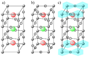
Figure 1: (Color online) Crystal structure of YBa₂Cu₃O_6+y. Grey and open circles are copper and oxide atoms, respectively. Additionally, oxygen atoms are divided into three groups: from fully oxidized copper-oxide layers (O_p), apical (O_ap), from oxygen deficient layers (O_b1, O_b2). Effect on oxygen doping is also shown: a) $y=0$ – O_b1 and O_b2 sites are empty; b) $y\in\left(0,1\right)$ – O_b1 and O_b2 sites occupied in random or ordered manner, depending on actual value of $y$; c) $y=1$ – oxygen is ordered forming chains: all O_b1 sites are occupied and O_b2 sites are empty.

Binding of electrons into pairs is essential in forming the superconducting state, however its remarkable properties–zero resistance and Meissner effect–require phase coherence among the pairs as well. While the phase order is unimportant for determining the value of the transition temperature $T_{c}$ in conventional BCS superconductors, in materials with low carrier density such as high-T_c oxide superconductors, phase fluctuations may have a profound influence on low temperature properties.Phase_fluctuations Measurements of the frequency-dependent conductivity, in the frequency range 100-600 GHz, show that phase correlations indeed persist above $T_{c}$, where the phase dynamics is governed by the bare microscopic phase stiffnesses.Phase_stiffnesses As a result, for underdoped cuprate superconductors, the conventional ordering of binding and phase stiffness energies appears to be reversed. Thus, the issue how phase correlations develop is a central problem of high-$T_{c}$ superconductivity. Furthermore, it was directly shown that integrating the electronic degrees of freedom out in $t$-$t^{{}^{\prime}}$-$U$-$J$ Hubbard model, which is believed to correctly describe strongly interacting systems, leads to phase-only description of superconductivity.t_t_U_J

In the present paper, we propose a semi-microscopic model of YBCO, which is founded on microscopic phase stiffnesses that set the characteristic energy scales: in-plane $J_{\|}$ and inter-plane $J_{\bot}$ couplings of CuO₂ layers, in-plane $J_{\|}^{{}^{\prime}}$ coupling of basal planes and inter-plane $J_{\bot}^{{}^{\prime}}$ coupling between neighboring basal and CuO₂ planes. Additionally, the model contains a parameter $\eta$, which controls anisotropy of $J_{\|}^{{}^{\prime}}$ gradually turning off basal in-plane coupling along $b$ direction while $\eta$ changes from 1 to 0. Using our previous results,OurPrevious we model values of in-plane phase stiffnesses as a function of oxygen amount to reproduce YBCO phase diagram and to elucidate the origin of the 60-K plateau. Our approach goes beyond the mean field level and is able to capture both the effects of phase fluctuations and huge anisotropy on the superconducting phase transition.

The outline of the reminder of the paper is as follows. In Section II we construct an anisotropic three-dimensional XY model. Furthermore, we solve it in the spherical approximation with the help of the transfer matrix method and obtain a dependence of the critical temperature on model parameters: $T_{c}=T_{c}\left(J_{\|},\,J_{\bot},\,J_{\|}^{{}^{\prime}},\,J_{\bot}^{{}^{\prime}},\,\eta\right)$. Subsequently, in Section III we elaborate on influence of oxygen ordering on $T_{c}$. We model values of in-plane phase stiffnesses as a function of oxygen amount and determine values of model parameters for which the YBCO phase diagram can be reproduced. In Section IV, relying on experimental data unveiling that oxygen doping of YBCO may introduce significant charge imbalance between CuO₂ planes and other oxygen sites, we show that the former are underdoped, while the latter – strongly overdoped almost in the whole region of oxygen doping in which YBCO is superconducting. Finally, in Section V we summarize the conclusions to be drawn from our work.

II Model

Since, in underdoped high-temperature superconductors, two temperature scales of short-length pairing correlations and long-range superconducting order seem to be well separated,EmeryKivelson we consider the situation, in which local superconducting pair correlations are established and the relevant degrees of freedom are represented by phase factors $0\leq\varphi_{\ell}\left(\mathbf{r}_{i}\right)<2\pi$ placed in a lattice with nearest neighbor interactions. In our notation, $\mathbf{r}_{i}$ numbers lattice sites within $\ell$-th $ab$ plane. The system becomes superconducting once U(1) symmetry group governing the $\varphi_{\ell}\left(\mathbf{r}_{i}\right)$ factors is spontaneously broken and the non-zero value of $\left\langle e^{i\varphi_{\ell}\left(\mathbf{r}_{i}\right)}\right\rangle$ appears signaling the long-range phase order. The Hamiltonian that we consider consists of four parts

$$H\left[\varphi\right]=H_{\|}+H_{\bot}+H_{\|}^{{}^{\prime}}+H_{\bot}^{{}^{\prime}}$$ (1)

containing various microscopic phase stiffnesses representing characteristic energy scales present in YBCO (see, Fig. 2) :

1. in-plane coupling $J_{\|}>0$ within CuO₂ layers:

   $$H_{\|} = -J_{\|}\sum_{\ell}\sum_{i<j}\left\{\cos\left[\varphi_{3\ell}\left(\mathbf{r}_{i}\right)-\varphi_{3\ell}\left(\mathbf{r}_{j}\right)\right]\right.$$ (2)

   $$+\left.\cos\left[\varphi_{3\ell+1}\left(\mathbf{r}_{i}\right)-\varphi_{3\ell+1}\left(\mathbf{r}_{j}\right)\right]\right\};$$

2. inter-plane coupling $J_{\bot}>0$ between neighboring CuO₂ layer:

   $$H_{\bot} = -J_{\bot}\sum_{\ell}\sum_{i<j}\cos\left[\varphi_{3\ell}\left(\mathbf{r}_{i}\right)-\varphi_{3\ell+1}\left(\mathbf{r}_{i}\right)\right];$$ (3)

3. in-plane coupling $J_{\|}^{{}^{\prime}}>0$ within basal planes, which can be gradually turned off along $b$ direction by anisotropy parameter $\eta\in\left[0,1\right]$ to simulate oxygen ordering:

   $$H_{\|}^{{}^{\prime}} = -J_{\|}^{{}^{\prime}}\sum_{\ell}\sum_{i}\sum_{j=-1,1}\left\{\cos\left[\varphi_{\ell}\left(\mathbf{r}_{i}\right)-\varphi_{\ell}\left(\mathbf{r}_{i}+j\hat{a}\right)\right]\right.$$ (4)

   $$+\left.\eta\cos\left[\varphi_{\ell}\left(\mathbf{r}_{i}\right)-\varphi_{\ell}\left(\mathbf{r}_{i}+j\hat{b}\right)\right]\right\};$$

4. inter-plane coupling $J_{\bot}^{{}^{\prime}}>0$ between adjacent CuO₂ layer and basal plane:

   $$H_{\bot}^{{}^{\prime}} = -J_{\bot}^{{}^{\prime}}\sum_{\ell}\sum_{i<j}\left\{\cos\left[\varphi_{3\ell+1}\left(\mathbf{r}_{i}\right)-\varphi_{3\ell+2}\left(\mathbf{r}_{i}\right)\right]\right.$$ (5)

   $$+\left.\cos\left[\varphi_{3\ell+2}\left(\mathbf{r}_{i}\right)-\varphi_{3\ell+3}\left(\mathbf{r}_{i}\right)\right]\right\}.$$

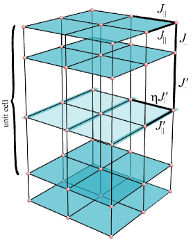
Figure 2: (Color online) Structure of the YBCO superconductor. Basal plane is in the middle of the picture with in-plane microscopic phase stiffness $J_{\|}^{{}^{\prime}}$, which can be strongly anisotropic when $\eta$ parameter is small (or isotropic for $\eta=1$). Basal plane coupling with neighboring CuO₂ planes is given by $J_{\bot}^{{}^{\prime}}$. In-plane and inter-plane microscopic phase stiffnesses of CuO₂ layers are $J_{\|}$ and $J_{\bot}$, respectively.

The indices $i,j$ go from $1$ to $N_{\|}$ being the number of sites in a plane, $\ell=1,...,N_{\bot}/3$, where $N_{\bot}$ denotes the number of layers and $N=N_{\|}N_{\bot}$ is the total number of sites. The partition function of the system reads:

$$Z=\int_{0}^{2\pi}\prod_{\ell,i}d\varphi_{\ell}\left(\mathbf{r}_{i}\right)e^{-\beta H\left[\varphi\right]},$$ (6)

where $\beta=1/k_{B}T$ with $T$ being the temperature. Introducing two-dimensional vectors $\mathbf{S}_{\ell}\left(\mathbf{r}_{i}\right)=\left[S_{x\ell}\left(\mathbf{r}_{i}\right),\,S_{y\ell}\left(\mathbf{r}_{i}\right)\right]$ of the unit length $\mathbf{S}_{\ell}^{2}\left(\mathbf{r}_{i}\right)=S_{x\ell}^{2}\left(\mathbf{r}_{i}\right)+S_{y\ell}^{2}\left(\mathbf{r}_{i}\right)=1$ defined by $\mathbf{S}_{\ell}\left(\mathbf{r}_{i}\right)=\left[\cos\varphi_{\ell}\left(\mathbf{r}_{i}\right),\sin\varphi_{\ell}\left(\mathbf{r}_{i}\right)\right],$ the Hamiltonian can be expressed in a vector form and the partition function written as:

$$Z=\int_{0}^{2\pi}\left\{\prod_{\ell,i}d^{2}\mathbf{S}_{\ell}\left(\mathbf{r}_{i}\right)\delta\left[\mathbf{S}_{\ell}^{2}\left(\mathbf{r}_{i}\right)-1\right]\right\}e^{-\beta H\left[S\right]},$$ (7)

where the unit length constraint ($\mathbf{S}_{\ell}^{2}\left(\mathbf{r}_{i}\right)=1$) is introduced by the set of Dirac-$\delta$ functions. Unfortunately, the partition function in Eq. (6) cannot be calculated exactly. However, the model becomes solvable, while the rigid length constraint in Eq. (7) is replaced by a weaker spherical closure relationSphericalModel

$$\delta\left[\mathbf{S}_{\ell}^{2}\left(\mathbf{r}_{i}\right)-1\right]\,\,\,\rightarrow\,\,\,\delta\left[\frac{1}{N}\sum_{i,\ell}\mathbf{S}_{\ell}^{2}\left(\mathbf{r}_{i}\right)-1\right].$$ (8)

Introducing different microscopic phase stiffnesses for CuO₂ and basal planes breaks translational symmetry along $c$ axis, since the inter-plane and in-plane couplings vary with period of $3$, when moving from one plane to another. As a result, standard way of diagonalizing the Hamiltonian using three-dimensional Fourier transform of variables ($\mathbf{S}_{\ell}\left(\mathbf{r}_{i}\right)$ in this case) fails, because of the lack of complete translational symmetry: To overcome this difficulty, we implement a combination of two-dimensional Fourier transform for in-plane vector variables

$$\mathbf{S}_{\ell}\left(\mathbf{r}_{i}\right)=\frac{1}{N_{\|}}\sum_{\mathbf{k}}\mathbf{S}_{\mathbf{k}\ell}e^{-i\mathbf{kr}_{i}}.$$ (9)

and transfer matrix method for one-dimensional decorated structure along $c$-axis.DecoratedLattice This former operation diagonalizes all terms in the Hamiltonian in Eq. (1) with respect to $\mathbf{k}$, leaving the dependence on layer index $\ell$ unchanged. Therefore, the partition function can be written in the form:

$$Z = \int_{-\infty}^{+\infty}\frac{d\lambda}{2\pi i}\exp\left\{N\lambda+\frac{1}{2}\ln\int_{-\infty}^{+\infty}\prod_{\mathbf{k},\ell}d^{2}\mathbf{S}_{\mathbf{k}\ell}\right.$$ (10)

$$\times\left.\exp\left[-\frac{1}{N_{\|}}\sum_{\mathbf{k},\ell,\ell^{\prime}}\mathbf{S}_{\mathbf{k}\ell}A_{N_{\bot}}^{\ell\ell^{\prime}}\left(\mathbf{k}\right)\mathbf{S}_{-\mathbf{k}\ell^{\prime}}\right]\right\},$$

where $A_{N_{\bot}}^{\ell\ell^{\prime}}\left(\mathbf{k}\right)$ is an element of a square $N_{\bot}\times N_{\bot}$ band matrix, appearing as a result of non-trivial coupling structure along $c$-direction:

$$\begin{array}[]{cc}&\\ A_{N_{\bot}}\left(\mathbf{k}\right)=&\left[\begin{tabular}[]{cccccccc}\cline{1-3}\cr\vrule\lx@intercol\hfil$\lambda-\frac{\beta J_{\|}\left(\mathbf{k}\right)}{2}$\hfil\lx@intercol &$-\frac{\beta J_{\bot}^{{}^{\prime}}}{2}$&\lx@intercol\hfil$0$\hfil\lx@intercol\vrule\lx@intercol&$0$&$\cdots$&$0$&$0$&$0$\\ \vrule\lx@intercol\hfil$-\frac{\beta J_{\bot}^{{}^{\prime}}}{2}$\hfil\lx@intercol&$\lambda-\frac{\beta J_{\|}^{{}^{\prime}}\left(\mathbf{k}\right)}{2}$&\lx@intercol\hfil$-\frac{\beta J_{\bot}^{{}^{\prime}}}{2}$\hfil\lx@intercol\vrule\lx@intercol&$0$&$\cdots$&$0$&$0$&$0$\\ \vrule\lx@intercol\hfil$0$\hfil\lx@intercol&$-\frac{\beta J_{\bot}^{{}^{\prime}}}{2}$&\lx@intercol\hfil$\lambda-\frac{\beta J_{\|}\left(\mathbf{k}\right)}{2}$\hfil\lx@intercol\vrule\lx@intercol&\fcolorbox[rgb]{0.9,0.9,0.9}{0.9,0.9,0.9}{$-\frac{\beta J_{\bot}}{2}$}&$\cdots$&$0$&$0$&$0$\\ \cline{1-4}\cr$0$&$0$&$\overset{\vspace{0.1em}}{\fcolorbox[rgb]{0.9,0.9,0.9}{0.9,0.9,0.9}{$-\frac{\beta J_{\bot}}{2}$}}$&\vrule\lx@intercol\hfil$\lambda-\frac{\beta J_{\|}\left(\mathbf{k}\right)}{2}$\hfil\lx@intercol&$\ddots$&$\vdots$&$\vdots$&$\vdots$\\ $\vdots$&$\vdots$&$\vdots$&$\ddots$&\lx@intercol\hfil$\lambda-\frac{\beta J_{\|}\left(\mathbf{k}\right)}{2}$\hfil\lx@intercol\vrule\lx@intercol&\fcolorbox[rgb]{0.9,0.9,0.9}{0.9,0.9,0.9}{$-\frac{\beta J_{\bot}}{2}$}&$0$&$0$\\ \cline{5-8}\cr$0$&$0$&$0$&$\cdots$&$\overset{\vspace{0.1em}}{\fcolorbox[rgb]{0.9,0.9,0.9}{0.9,0.9,0.9}{$-\frac{\beta J_{\bot}}{2}$}}$&\vrule\lx@intercol\hfil$\lambda-\frac{\beta J_{\|}\left(\mathbf{k}\right)}{2}$\hfil\lx@intercol &$-\frac{\beta J_{\bot}^{{}^{\prime}}}{2}$&\lx@intercol\hfil$0$\hfil\lx@intercol\vrule\lx@intercol\\ $0$&$0$&$0$&$\cdots$&$0$&\vrule\lx@intercol\hfil$-\frac{\beta J_{\bot}^{{}^{\prime}}}{2}$\hfil\lx@intercol&$\lambda-\frac{\beta J_{\|}^{{}^{\prime}}\left(\mathbf{k}\right)}{2}$&\lx@intercol\hfil$-\frac{\beta J_{\bot}^{{}^{\prime}}}{2}$\hfil\lx@intercol\vrule\lx@intercol\\ $0$&$0$&$0$&$\cdots$&$0$&\vrule\lx@intercol\hfil$0$\hfil\lx@intercol&$-\frac{\beta J_{\bot}^{{}^{\prime}}}{2}$&\lx@intercol\hfil$\underset{\vspace{0.1em}}{\lambda-\frac{\beta J_{\|}\left(\mathbf{k}\right)}{2}}$\hfil\lx@intercol\vrule\lx@intercol \\ \cline{6-8}\cr\end{tabular}\right].\\ &\hfill\hfil\end{array}$$ (11)

where:

$$J_{\|}\left(\mathbf{k}\right) = 2J_{\|}\left[\cos\left(ak_{x}\right)+\cos\left(bk_{y}\right)\right],$$

$$J_{\|}^{{}^{\prime}}\left(\mathbf{k}\right) = 2J_{\|}^{{}^{\prime}}\left[\cos\left(ak_{x}\right)+\eta\cos\left(bk_{y}\right)\right]$$ (12)

and $\lambda$is a Lagrange multiplier introduced by representing the Dirac-$\delta$ function in a spectral form $\delta\left(x\right)=\int_{-\infty}^{+\infty}d\lambda/2\pi i\exp\left(-\lambda x\right)$. The problem reduces then to evaluation of a determinant of the $A_{N_{\bot}}^{\ell\ell^{\prime}}\left(\mathbf{k}\right)$ matrix (for technical details, we refer readers to Ref. [OurPrevious, ]).

The partition function in Eq. (10) can be written as:

$$Z=\int_{-\infty}^{+\infty}\frac{d\lambda}{2\pi i}\exp\left[-N\beta f\left(\lambda\right)\right].$$ (13)

In the thermodynamic limit $N\rightarrow\infty$ the dominant contribution to the integral in Eq. (13) comes from the saddle point $\lambda=\lambda_{0}$ of $f\left(\lambda\right)$:

$$\left.\frac{\partial f\left(\lambda\right)}{\partial\lambda}\right|_{\lambda=\lambda_{0}}=0$$ (14)

and where $f\left(\lambda=\lambda_{0}\right)$ becomes a free energy. In the spherical model, the emergence of the critical point is signaled by divergence of the order parameter susceptibility:

$$G^{-1}\left(\mathbf{k}=0\right)=0,$$ (15)

where $G^{-1}\left(\mathbf{k}\right)\equiv\left\langle\mathbf{S}_{\mathbf{k},\ell}\mathbf{S}_{\mathbf{-k},\ell}\right\rangle$ and $\left\langle...\right\rangle$ is the statistical average. Eq. (15) determines the value of the Lagrange multiplier $\lambda$. Consequently, the free energy of the system reads:

$$f = \frac{\lambda}{\beta}-\frac{1}{3\beta}\int_{-\frac{\pi}{a}}^{+\frac{\pi}{a}}\int_{-\frac{\pi}{b}}^{+\frac{\pi}{b}}\frac{dk_{x}dk_{y}}{\left(2\pi\right)^{2}/\left(ab\right)}\ln\left[\frac{1}{16}\left(\left\{\left(\beta J_{\bot}\right)^{2}-\left[\Lambda\left(\mathbf{k}\right)\right]^{2}\right\}\Lambda^{{}^{\prime}}\left(\mathbf{k}\right)+2\left(\beta J_{\bot}^{{}^{\prime}}\right)^{2}\Lambda\left(\mathbf{k}\right)\right)\right.$$ (16)

$$\left.+\sqrt{\left\{\left(\beta J_{\bot}\right)^{2}-\left[\Lambda\left(\mathbf{k}\right)\right]^{2}\right\}\left\{\left(\beta J_{\bot}\right)^{2}\left[\Lambda^{{}^{\prime}}\left(\mathbf{k}\right)\right]^{2}-\left[2\left(\beta J_{\bot}^{{}^{\prime}}\right)^{2}-\Lambda\left(\mathbf{k}\right)\Lambda^{{}^{\prime}}\left(\mathbf{k}\right)\right]^{2}\right\}}\right],$$

where functions $\Lambda\left(\mathbf{k}\right)=\beta J_{\|}\left(\mathbf{k}\right)-2\lambda_{0}$ and $\Lambda^{{}^{\prime}}\left(\mathbf{k}\right)=\beta J_{\|}^{{}^{\prime}}\left(\mathbf{k}\right)-2\lambda_{0}$. The Lagrange multiplier reads:

$$\lambda_{0}=\frac{\beta}{4}\left\{4J_{\|}+2J_{\|}^{{}^{\prime}}\left(1+\eta\right)+J_{\bot}+\sqrt{8\left(J_{\bot}^{{}^{\prime}}\right)^{2}+\left[J_{\bot}+4J_{\|}+2J_{\|}^{{}^{\prime}}\left(1-\eta\right)\right]^{2}}\right\}.$$ (17)

Finally, the Eq. (14) leads to expression for the critical temperature:

$$\beta_{c}=\frac{2}{3}\int_{-1}^{+1}d\xi\int_{-1}^{+1}d\zeta\rho\left(\xi\right)\rho\left(\zeta\right)\frac{2\left(J_{\bot}^{{}^{\prime}}\right)^{2}+\left(J_{\bot}\right)^{2}-4\alpha\left(\alpha+2\alpha^{{}^{\prime}}\right)}{\sqrt{\left\{\left[\left(J_{\bot}^{{}^{\prime}}\right)^{2}-2\alpha\alpha^{{}^{\prime}}\right]^{2}-\left(J_{\bot}\alpha^{{}^{\prime}}\right)^{2}\right\}\left[\left(2\alpha\right)^{2}-J_{\bot}^{2}\right]}},$$ (18)

where $\alpha\equiv\lambda_{0}/\beta-J_{\|}\left(\xi+\zeta\right)$, $\alpha^{{}^{\prime}}\equiv\lambda_{0}/\beta-J_{\|}^{{}^{\prime}}\left(\xi+\eta\zeta\right)$ and $\rho\left(\varepsilon\right)$ is a density of states of the chain (one-dimensional) lattice given by:

$$\rho\left(\varepsilon\right)=\frac{1}{\pi}\frac{1}{\sqrt{1-\varepsilon^{2}}}\Theta\left(1-\left|\varepsilon\right|\right),$$ (19)

and $\Theta\left(x\right)$ is the unit-step function.

III Influence of oxygen ordering on the critical temperature

The result in Eq. (18) provides us with a tool to analyze the influence of anisotropy and characteristic energy scales present in YBCO on the critical temperature. However, in order to describe YBCO phase diagram, it is necessary to connect the model parameters with amount of oxygen doping. In our previous paper we have proposed a phenomenological dependence of in-plane microscopic phase stiffness of CuO₂ plane on charge (hole) concentration, which appeared to successfully describe properties of superconducting homologous series:OurPrevious

$$J_{\|}\left(\delta\right)=\left\{\begin{array}[]{l}J_{\|}\left[1-\frac{1}{0.01}\left(\delta-0.15\right)^{2}\right]\,\,\mathrm{for}\,\,0.05<\delta<0.025\\ 0\,\,\,\mathrm{for}\,\,\delta\leq 0.05\,\,\mathrm{or\,\,\delta\geq 0.25}.\end{array}\right.$$ (20)

To adapt it to the present model it is necessary to relate oxygen amount to charge concentration in CuO₂ planes, since YBCO phase diagram is presented as an oxygen doping function of temperature. This relation was experimentally determined by Tallon, et at. and found out to be roughly linear in the superconducting region (charge concentration changes from $\delta=0.05$ for $y=0.4$ to $\delta=0.17$ for $y=1$).GenericBehaviorYBCO Consequently, the in-plane phase stiffness from Eq. (20) expressed as a function of oxygen amount reads $J_{\|}\left(y\right)=J_{\|}g\left(y\right)$, where:

$$g\left(y\right)=\left\{\begin{array}[]{l}1-\frac{1}{0.55^{2}}\left(y-0.95\right)^{2}\,\,\mathrm{for}\,\,0.4\leq y\leq 1\\ 0\,\,\,\mathrm{for}\,\,\mathrm{y\leq 0.4}.\end{array}\right.$$ (21)

Although, it is usually stated in the literature, T-O phase transition and emergence of superconductivity in YBCO are not simultaneous in terms of doping.OTPhaseTransition Thus, we suggest the following scenario describing the phase diagram of YBCO (see, Fig. 4): with increasing oxygen doping (starting from $y=0$), the onset of superconductivity is reached ($y=0.4$). The critical temperature is rising up to a point, in which T-O phase transition occurs ($y=0.5$). For higher dopings, oxygen chains start to form. That results in interactions in basal planes becoming more one-dimensional, thus phase fluctuations rise significantly and enough to keep the critical temperature constant. Further, while all the oxygen is ordered in chains, the critical temperature roughly follows in-plane phase stiffness $J_{\|}$ dependence on doping reaching its maximum value of $93\mathrm{K}$ for $y=0.95$ and dropping slightly later.

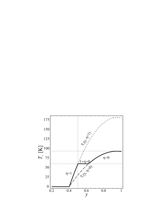
Figure 3: Construction of YBCO phase diagram within presented model: curves for $T_{c}\left(y,\,\eta\right)$ for disordered ($\eta=1$) and fully ordered ($\eta=0$) oxygen set limits for the actual phase diagram. For low dopings ($y<0.5$) interactions in the basal planes are isotropic and $T_{c}\left(y\right)$ dependence falls on $\eta=1$ curve. On the other hand, for $y=1$, all added oxygen atoms form chains and the critical temperature reaches the other limit of $\eta=0$. Plateau region is a crossover between those two regimes in which variable value of $\eta$ keeps $T_{c}$ conA. J. Leggett

Figure 4: Affiliation: Department of Physics, University of Illinois at Urbana-Champaign, Urbana, Illinois 61801, USAstant.

In order to realize this scenario within the presented model it is necessary to fix values of model parameters $J_{\|}$, $J_{\|}^{{}^{\prime}}$, $J_{\bot}$, $J_{\bot}^{{}^{\prime}}$ and find a dependence of $\eta$ on doping $y$, which would results in constant critical temperature in the plateau region of the phase diagram. We assume that doping dependence of $J_{\|}$ and $J_{\|}^{{}^{\prime}}$ are given by Eq. (e21), and, for simplicity, $J_{\bot}\equiv J_{\bot}^{{}^{\prime}}$. Experimental data for anisotropy of penetration depth in YBCO provide us with ratio of $J_{\bot}/J_{\|}=\lambda_{ab}^{2}/\lambda_{c}^{2}\simeq 100$.PenetrationDepth Furthermore, values of $J_{\|}$ and $J_{\|}^{{}^{\prime}}$ can be deduced from the ratio of expressions for the critical temperatures (see, Fig. 4) for plateau ($60K$) and optimum doping ($93K$):

$$\frac{T_{c}\left(J_{\|,}\,J_{\|}^{{}^{\prime}},\,y=0.5,\,\eta=1\right)}{T_{c}\left(J_{\|,}\,J_{\|}^{{}^{\prime}},\,y=0.95,\,\eta=0\right)}=\frac{60}{93}.$$ (22)

Finally, dependence of oxygen ordering on doping $\eta\left(\delta\right)$ can be found numerically for calculated values of model parameters ($J_{\|}=19.32\textrm{meV}$, $J_{\|}^{{}^{\prime}}=33.81\mathrm{meV}$, $J_{\bot}=J_{\bot}^{{}^{\prime}}=0.58\mathrm{meV}$) and it can by approximated by the expression:

$$\eta\left(\delta\right)=\frac{1}{3}\left[\left(2-2\delta\right)^{15.2}+\left(2-2\delta\right)^{7.9}+\left(2-2\delta\right)^{3.6}\right].$$ (23)

The resulting phase diagram is presented in Fig. 5 (thick solid line) along with experimental results, for comparison. It is clearly seen that the procedure reproduces characteristic features of YBCO phase diagram: 60-K plateau, 93K maximum critical temperature with small overdoped region. However, trying to fit experimental data better, we have performed more exact (non-linear) approximation of data from Ref. [GenericBehaviorYBCO, ] that lead to doping dependence of in-plane phase stiffness $J_{\|}\left(y\right)$. Corresponding phase diagram is also presented in Fig. 5 as thick dashed line. It does not provide any new quality increasing the width of 60-K plateau only very slightly, thus it is reasonable to use simpler form of $J_{\|}\left(y\right)$ dependence, as in Eq. (21). It can be also noticed that the model predicts 60-K plateau to be a little bit narrower and moved toward lower doping region than experimental results show. It can be argued that since it is very hard to control the amount of oxygen in YBCO precisely, some measurements, especially based on multigrain powder samples, can be inaccurate. However newer results are based on un-twinned single crystals and seem to be reliable, also because of good consistence among different research groups.

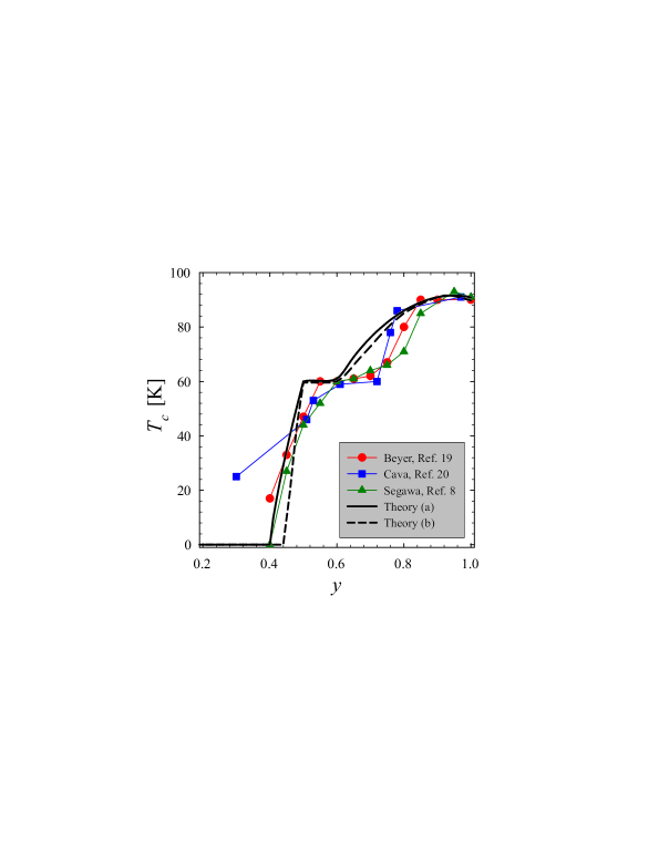
Figure 5: (Color online) Comparison of experimental phase diagrams of YBCO with results of the presented model for a) linear and b) non-linear (more exact) approximation of data of Tallon, et al. (see, Ref GenericBehaviorYBCO, ).

Unfortunately, the most serious flaw in the presented scenario are the actual values of model parameters required to reproduce experimental phase diagram. It is necessary for basal plane in-plane microscopic phase stiffness $J_{\|}^{{}^{\prime}}$ to be almost two times bigger than CuO₂ planes coupling $J_{\|}$. For more reasonable values $J_{\|}>J_{\|}^{{}^{\prime}},\,J_{\bot},\,J_{\bot}^{{}^{\prime}}$, the influence of anisotropy in basal planes is almost negligible. For example for $J_{||}=J_{\|}^{{}^{\prime}}=J$, $J_{\bot}^{{}^{\prime}}=0.1J$ and $J_{\bot}=0.01J$ with $J=19.3\mathrm{meV}$, the ratio of critical temperatures for systems with anisotropic ($\eta=0$) and isotropic ($\eta=1$) interactions in basal planes reads:

$$\frac{T_{c}\left(\eta=0\right)}{T_{c}\left(\eta=1\right)}=0.949.$$ (24)

Similarly, for $J_{||}=J_{\|}^{{}^{\prime}}=J$, $J_{\bot}^{{}^{\prime}}=0.1J$ and $J_{||}=J$, $J_{||}^{{}^{\prime}}=J_{\bot}^{{}^{\prime}}=0.5J$ and $J_{\bot}=0.1J$ the ratio is $0.983$. The influence of basal plane anisotropy is too small to noticeably change the critical temperature until in-plane phase stiffness $J_{\|}^{{}^{\prime}}$ is increased to be higher than $J_{\|}$. This, however, does not seem to be reasonable from physical point of view. Evolution of the phase diagram with changing ratio of $J_{\|}^{{}^{\prime}}/J_{\|}$ is presented in Fig. 6. When the ratio is being decreased, the plateau region is disappearing. To summarize, we find it rather unlikely that oxygen ordering into chains alone can explain the existence of 60-K plateau.

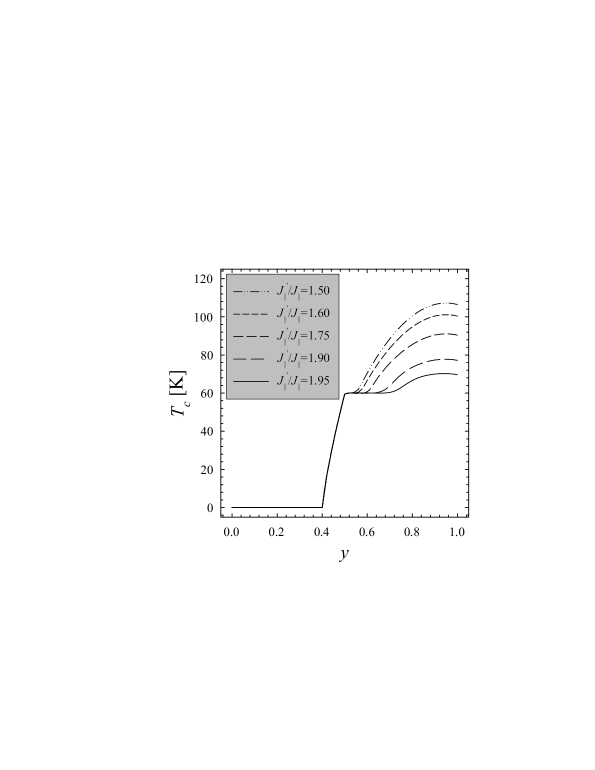
Figure 6: Comparison of phase diagrams for various ratios of $J_{\|}^{{}^{\prime}}/J_{\|}$. Plots are normalized to have the critical temperature of the plateau region equal to $60\mathrm{K}$.

IV Influence of doping imbalance on the critical temperature

YBCO can be doped not only by adding the oxygen atoms, but also by substituting three-valent Yttrium atoms with two-valent Calciums. This introduces holes directly to CuO₂ planes leaving apical and chain sites untouched:Apical_oxygen even though the charge concentration within copper-oxide planes is high enough, lack of doping of apical sites results in interplane coupling being small and the onset of superconductivity is not reached. This suggests that charge concentration within apical sites along with basal plane sites and CuO₂ layers can be significantly different. Similarly, as Yttrium substitution can lead to introduction of holes exclusively into CuO₂ planes, one can imagine that increasing of oxygen amounts changes charge concentration primarily in the chain regions and only some of the charges are transported to the copper-oxide layers. In fact, this scenario has been confirmed by means of site-specific X-ray absorption spectroscopy.Apical_oxygen Because overdoping of some regions of YBCO could provide a factor decreasing the critical temperature with increasing oxygen doping and thus leading to the 60-K plateau, we want to investigate such a possibility within presented model.

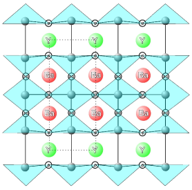
Figure 7: (Color online) YBa₂Cu₃O₇ structure with copper-oxide chains fully formed.

First, we want to emphasize the high significance of apical site doping. Analyzing a projection of the YBCO structure on $a-c$ plane (presented in Fig. 7), it can be noticed that a set of chains differs from full copper-oxide layer only by a lack of oxygens between CuO₂ planes. Thus one can expect that the microscopic phase stiffnesses $J_{\bot}^{{}^{\prime}}$ related to apical sites and the one within basal planes $J_{\|}^{{}^{\prime}}$ are of the order of CuO₂ in-plane phase stiffness $J_{\|}$. This suggests it is reasonable to investigate the role of doping of apical and basal sites on the phase diagram of YBCO. To investigate this , we want to determine values of $J_{\|}^{{}^{\prime}}$ and $J_{\bot}^{{}^{\prime}}$ that would result in $T_{c}\left(y\right)$ dependence observed experimentally. For clarity, we assume that oxygen is fully ordered in chains to study the effect of charge imbalance alone. It is also necessary to model an influence of the number of vacancies in basal planes for $y<1$ on the in-plane phase stiffness $J_{\|}^{{}^{\prime}}$. This relation is unfortunately not obvious and it is hard to find any hint about it specific form. Thus, we start with a simple linear dependence $h\left(y\right)=y$, so : $J_{\|effective}^{{}^{\prime}}\left(y\right)=y^{\gamma}J_{\|}^{{}^{\prime}}\left(y\right)$ with $\gamma=1$.OxygenVacanciesComment Later, we choose different value of $\gamma=3/2$ and notice that although specific values of $J_{\|}^{{}^{\prime}}$ and $J_{\bot}^{{}^{\prime}}$ change, the qualitative results are the same and in reasonable agreement with experimental data.

Our procedure is as follows: we assume that anisotropy ratio between in-plane and inter-plane coupling among CuO₂ planes is equal to $J_{\bot}/J_{\|}=0.0136$,OurPrevious $\eta$ parameter is equal to $0$ (oxygen in basal planes is ordered along $a$ direction) and values of $J_{\|}^{{}^{\prime}}$ and $J_{\bot}^{{}^{\prime}}$ are equal and of the order of $J_{\|}$ (however $J_{\|}^{{}^{\prime}}$ is modified by chosen factor $h\left(y\right)=y^{\gamma}$). Providing values of $J_{\|}$, $J_{\bot}$ and $\eta$ into Eq. (18) along with experimentally obtained critical temperatures based on resistivity measurements from Ref. [YBCO_transport, ], we determine doping dependence of basal and apical microscopic phase stiffnesses. The results are presented in Fig. 8. Using expression in Eq. (20) it is also possible to calculate doping dependence of corresponding charge concentration (see, Fig. 9). As it is apparent, almost in the whole region of oxygen doping in which YBCO is superconducting, basal planes along with apical sites are overdoped while simultaneously CuO₂ planes are underdoped. While oxygen content is increased, this provides two counteracting factors, which may lead to rise of 60K plateau. Although specific relation of $J_{\|}^{{}^{\prime}}$ and $J_{\bot}^{{}^{\prime}}$ on $y$ is dependent on assumed factor $h\left(y\right)=y^{\gamma}$, the results are qualitatively similar and in reasonable agreement with experimental data (see stars, in Fig. 9).

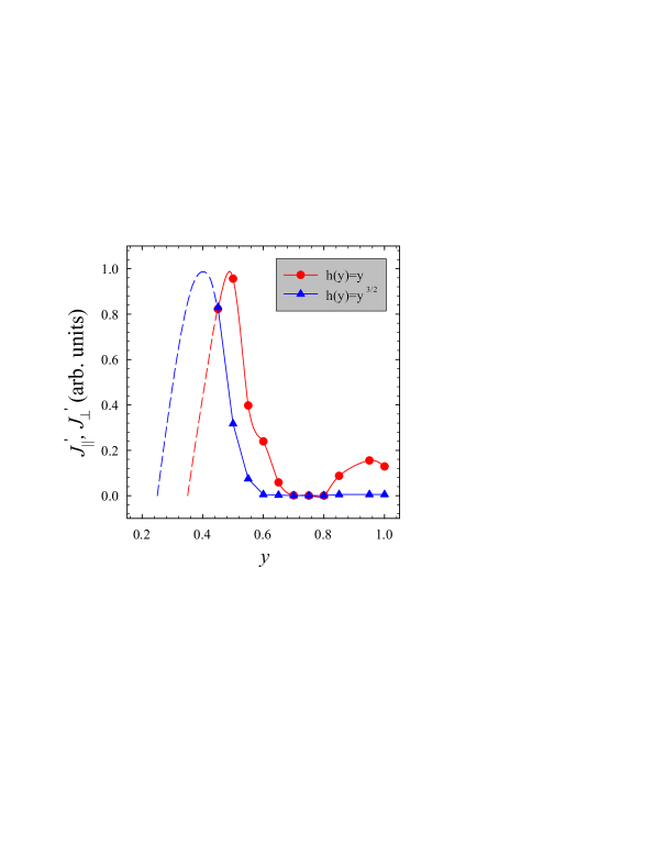
Figure 8: (Color online) Calculated dependence of $J_{\|}^{{}^{\prime}}$ and $J_{\bot}^{{}^{\prime}}$ on oxygen amount for various factors due to number of oxygen vacancies in copper-oxide chains. Dependences are normalized to have maximum value equal to 1. Dashed lines are guides for eye extending dependences beyond region where calculation was possible.

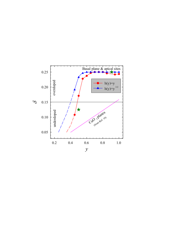
Figure 9: (Color online) Charge concentration within basal planes, apical sites and in CuO₂ planes. Stars denote experimental values of hole doping in basal planes and apical sites (from Ref. [Apical_oxygen, ]). Dashed lines are guides for eye extending dependences beyond region where calculation was possible.

V Summary and conclusions

We have considered a model of YBa₂Cu₃O_6+y to study the influence of oxygen ordering and doping imbalance on the critical temperature $T_{c}\left(y\right)$ and to elucidate a possible origin of well-known feature of YBCO phase diagram: the 60-K plateau. Motivated by the experimental evidence that the ordering of the phase degrees of freedom is responsible for the emergence of the superconducting state with long-range order, we focus on the “phase only” description of the high-temperature superconducting system. In our approach, the vanishing of the superconductivity with underdoping can be understood by the reduction of the in-plane phase stiffnesses and can be linked to the manifestation of Mott physics (no double occupancy due to the large Coulomb on-site repulsion) that leads to the loss of long-range phase coherence while moving toward half-filled limit ($y=0$). For doping $y=0$, the fixed electron number implies large fluctuations in the conjugate phase variable, which naturally translates into the reduction of the microscopic in-plane phase stiffnesses and destruction of the superconducting long-range order in this limit. In the opposite region of large $y$, the onset of a pair-breaking effect (at the pseudogap temperature $T^{*}$) can deplete the microscopic phase stiffnesses, thus reducing the critical temperature.

To this end, we have utilized a three-dimensional semi microscopic XY model with two-component vectors that involve phase variables and adjustable parameters representing microscopic phase stiffnesses and an anisotropy parameter. The model fully implements complicated energy scales present in YBCO also allowing for strong anisotropy within basal planes in order to simulate oxygen ordering. Applying spherical closure relation we have solved the phase XY model with the help of transfer matrix method and calculated $T_{c}$ for chosen system parameters. Furthermore, by making a physically justified assumption regarding the doping dependence of the microscopic phase stiffnesses we are able to recreate the phase diagram of YBCO and investigate the influence of oxygen ordering and doping imbalance on its shape. We determine that characteristic features of the phase diagram, i.e. 60-K plateau, can be recreated by effects of oxygen ordering. However, the specific values of the model parameters for which this result is obtained seem to be a little bit hard to justify. Furthermore, relying on experimental data unveiling that oxygen doping of YBCO may introduce significant charge imbalance between CuO₂ planes and other oxygen sites, we show that the former are underdoped, while the latter – strongly overdoped almost in the whole region of oxygen doping in which YBCO is superconducting. Increasing of the oxygen content provides then a natural mechanism of two counter acting factors that leads to emergence of 60-K plateau. Additionally, our result can provide an important contribution to solve a controversy of the symmetry of YBCO order parameter, for which various experiments give contradictory answers suggesting $d$ or $s$-wave (although the fact that YBCO is orthorhombic should also lead to order parameter being a mixture of $s$ and $d$-wave). OrderParam1 Furthermore, measurements of the complex conductivity of high quality YBCO crystals show a third peak in the normal conductivity at 80K along with enhanced pair conductivity below $\sim 60\mathrm{K}$.OrderParam2 Authors show that a single $d$-wave order parameter is insufficient to describe the data and successfully consider two-component model of superconductivity in YBCO. They claim that it would be tempting to assign the two superconducting components with the associated condensates residing on CuO₂ planes and chains, respectively, however they do not see any justification of such situation. Thus, our result can provide a natural answer for plausibility of such a scenario, in which $s$-wave component comes from overdoped chains and $d$-wave one – from underdoped CuO₂ planes.

- (1) M.K. Wu, J.R. Ashburn, C.J. Torng, P.H. Hor, R.L. Meng, L. Gao, Z.J. Huang, Y.Q. Wang, and C.W. Chu, Phys. Rev. Lett. 58, 908 (1987).
- (2) J.M.S. Skakle, Mater. Sci. Eng. R23, 1 (1998).
- (3) M. Merz, N. Nücker, P. Schweiss, S. Schuppler, C. T. Chen, V. Chakarian, J. Freeland, Y. U. Idzerda, M. Kläser, G. Müller-Vogt, and Th. Wolf, Phys. Rev. Lett. 80, 5192 (1998).
- (4) A. Ourmazd, J.C.H. Spence, Nature (London) 329, 425 (1987).
- (5) C. Chaillout, M.A. Alario-Franco, J.J. Capponi, J. Chenavas, J.L. Hodeau, and M. Marezio, Phys. Rev. B 36, 7118 (1987).
- (6) H.F. Poulsen, N.H. Andersen, J.V. Andersen, H. Bohrt, and O.G. Mouritsen, Nature (London) 349, 594 (1991).
- (7) Y. Yan, M.G. Blanchin, C. Picard, P. Gerdanian, J. Mater. Chem. 3, 603 (1993).
- (8) K. Segawa and Y. Ando, J. Low Temp. Phys. 131, 822 (2003).
- (9) V.J. Emery, and S.A. Kivelson, Nature (London) 374, 434 (1995).
- (10) J. Corson, R. Mallozzi, J. Orenstein, J. N. Eckstein, and I. Bozovic, Nature (London) 398, 221 (1999).
- (11) T.K. Kopeć, Phys. Rev. B 70, 054518 (2004).
- (12) T.A. Zaleski and T.K. Kopeć, Phys. Rev. B 71, 014519 (2005).
- (13) V. J. Emery, S. A. Kivelson, Nature 374, 434 (1995).
- (14) T. H. Berlin and M. Kac, Phys. Rev. 86, 821 (1952); H. E. Stanley, ibid. 176, 718 (1968); G. S. Joyce, Phys. Rev. 146, 349 (1966); G. S. Joyce, in Phase Transitions and Critical Phenomena, edited by C. Domb and M. S. Green (Academic, New York, 1972), Vol. 2, p. 375.
- (15) S. Fishman, T. A. L. Ziman, Phys. Rev. B 26, 1258 (1982).
- (16) J.L. Tallon, C. Bernhard, H. Shaked, R.L. Hitterman, and J.D. Jorgensen, Phys. Rev. B 51, R12911 (1995).
- (17) L. Li, S. Cao, F. Liu, W. Li, C. Chi, C. Jing, and J. Zhan, Physica C 418, 43 (2005).
- (18) C. Panagopoulos, J.R. Cooper, T. Xiang, G.B. Peacock, I. Gameson, P.P. Edwards, W. Schmidbauer, and J.W. Hodby, Physica C 282-287, 145 (1997).
- (19) R. Beyers, B.T. Ahn, G. Gorman, V.Y. Lee, S.S.P. Parkin, M.L. Ramirez, K.P. Roche, J.E. Vazquez, T.M. Gür, and R.A. Huggins, Nature (London) 340, 619 (1989).
- (20) R.J. Cava, B.Batlogg, C.H. Chen, E.A. Rietman, S.M. Zahurak, and D. Werder, Nature (London) 329, 423 (1987).
- (21) In order to find exact influence of number of oxygen vacancies in chains on it would be necessary to calculate doping-dependent anisotropic penetration depth and fine tune it to experimental results.
- (22) R. Combescot and X. Leyronas, Phys. Rev. Lett. 75, 3732 (1995), and references therein.
- (23) H. Srikanth, B.A. Willemsen, T. Jacobs, S. Sridhar, A. Erb, E. Walker, and R. Flükiger, Phys. Rev. B 55, R14733 (1997).