On different $q$-systems in nonextensive thermostatistics

Abstract

It is known that the nonextensive statistics was originally formulated for the systems composed of subsystems having same $q$. In this paper, the existence of composite system with different $q$ subsystems is investigated by fitting the power law degree distribution of air networks with $q$-exponential distribution. Then a possible extension the nonextensive statistics to different $q$ systems is provided on the basis of an entropy nonadditivity rule and an unnormalized expectation of energy.

PACS : 02.50.-r; 05.20.-y; 05.70.-a

1 Introduction

The starting point of the nonextensive statistics (NS) of Tsallis[1] is the entropy given by

$$S_{q}=\frac{\sum_{i=1}^{w}p_{i}^{q}-1}{1-q}$$ (1)

where the physical states are labelled by $i=1,2,...,w$, $q$ is a parameter characterizing the nonextensivity of the theory, and $p_{i}$ is the probability for the system to be found at state $i$. The application of the principle of maximum entropy under appropriate constraints can lead to power law distributions characterized by the so called $q$-exponential functionals[1, 2]. For example, for canonical ensemble under the constraints associated with probability normalization and average energy, we can have :

$$p_{i}=\frac{1}{Z_{q}}[1-(1-q)\beta E_{i}]^{1/1-q}\;\;\;[\cdot]>0$$ (2)

where $Z_{q}$ is the partition function, $E_{i}$ is the energy of a microstate $i$, and $\beta=\frac{\partial S_{q}}{\partial U_{q}}$ is the Lagrange multiplier associated with the average energy $U_{q}$. It is worth noticing that, due to the different formalisms of NS proposed in the past 15 years, the inverse temperature $\beta$ has been given several definitions in different formulation of NS. A comment on this subject was given in ref.[3]. In the present work, we consider the formulation with $\sum_{i=1}^{w}p_{i}=1$ and $U_{q}=\sum_{i=1}^{w}p_{i}^{q}E_{i}$ leading to the $q$-exponential distribution given by Eq.(2).

For a composite system $(A+B)$ whose joint probability $p_{i}(A+B)$ is given by the product of the probabilities of its subsystems having the same $q$, i.e., $p_{ij}(A+B)=p_{i}(A)p_{j}(B)$ (product joint probability-PJP), we have, from Eq.(1)

$$S_{q}(A+B)=S_{q}(A)+S_{q}(B)+(1-q)S_{q}(A)S_{q}(B)$$ (3)

and, from Eq.(2)

$$E_{ij}(A+B)=E_{i}(A)+E_{j}(B)+(q-1)\beta E_{i}(A)E_{j}(B)$$ (4)

Eqs.(3) and (4) prescribe the class of nonextensive systems to which NS may be applied. They are analogs (or generalizations) of the entropy and energy additivity in the conventional Boltzmann-Gibbs statistics (BGS) and can be considered as starting hypothesis of NS. It has been proved that[4, 5] Eq.(3) uniquely determines Tsallis entropy (given PJP) and that[6, 7] Eqs.(3) and (4) are a group of necessary conditions for the existence of thermal equilibrium and stationarity between nonextensive systems.

Among the fundamental questions about NS, an interesting one is about its validity for the systems containing subsystems with different $q$’s, as has been recently discussed by several authors[8, 9, 10]. The debate turns around the establishment of the zeroth law for nonextensive systems. As is well known, for equilibrium (and local equilibrium) systems, this law allows one to measure intensive variables like temperature and pressure and to relate them to other thermodynamic variables and functions. For other nonequilibrium systems, a relationship between intensive variables like zeroth law may also be necessary in order to maintain the links between different parts of a system through thermodynamic functions.

The applications of NS during the last years were often carried out for systems considered as a whole[11, 12, 13, 14]. So the question of composition of different $q$ subsystems did not arise. From theoretical point of view, hierarchically invariant NS, just like BGS, should have its place for the hierarchies that have about the same space-time scale and include essentially the same physics. An example is the networks to which application of NS has been considered[15]. Indeed, in the study the scientific collaboration networks[16] for example, if NS is successful for an international collaboration network, it is hoped that it holds also for the national or regional collaboration networks which compose the international one and possibly have different $q$’s. The reader will find below an example of this situation with the airline networks.

A possible extension of NS was briefly mentioned in [3]. In what follows, after demonstration of the existence of different $q$ subsystems and composite systems all obeying $q$-exponential distribution given by Eq.(2), a detailed development of this extension is given by replacing Eq.(3) with a new nonadditivity rule and by establishing the zeroth law with the unnormalized expectation of energy as mentioned above. It is expected that this result may serves as a possible mathematical complement of the work of [8, 17] where the authors studied the possibility of measuring the dynamical temperature of a non Boltzmannian systems ($q\neq 1$) in stationary states with a Boltzmannian thermometer ($q=1$). This work is not complete as a generalization of the whole NS theory to different $q$ systems because the validity of this approach for the normalized expectation based on escort probability[2], widely usd in NS, is still open for investigation.

2 An example of different $q$-systems

Here we present an application of NS to both a total system and its subsystems, in order to show that the two subsystems and the composite system all have $q$-exponential distribution but with different $q$’s. Two subsystems are China air network and US air network. The composite system is the air network which includes the airports in both countries.

In the air network, airports are viewed as nodes. The connections between airports are simply represented by flights. In the terminology of network, the degree $k$ of a certain airport means it has flights with $k$ other airports in the same network. A very important quantity is the distribution of $k$, $p(k)$, called degree distribution, which tells the probability of finding an airport with degree $k$. Apparently, the degree distribution specifies the topology of the network investigated. For example, there are many different types of networks, classified by their respective degree distributions, scale-free, random, and so on.

China air network consists of 128 major airports [18] and for US air network, that number is 215 [19]. Hence the composite system of China and US air network has 343 major airports. Besides all the flights of the two original subsystems, the newly composed system also includes a few international flights, such as the one from Beijing to New York, etc. Since the number of international flights is much less than that of national ones, constructing the composite system can be viewed as adding two independent subsystems.

Two main reasons may account for why we can use the Tsallis distribution to fit the degree distribution. First, the air network is not a system which can reach the state of equilibrium. Like many other complex systems in evolution, the air network consists of many units having complicated interplay (interactions). Second, the observations from [18] and [19] have suggested that the degree distributions behave more like power-laws (in two regimes). As we know, Tsallis statistics provides a way to generate naturally power-law distribution and has been satisfactorily used for fitting certain distribution functions of complex systems[20, 21].

Our first idea was to fit the observed degree distributions separately in the two regimes with the following function

$$p(k)=\frac{[1-(1-q_{i})\beta_{i}k]^{\frac{1}{1-q_{i}}}}{\sum_{k}[1-(1-q_{i})\beta_{i}k]^{\frac{1}{1-q_{i}}}},i=1,2$$ (5)

where $q_{1},\beta_{1}$ and $q_{2},\beta_{2}$ are the parameters for the small $k$ and large $k$ regimes, respectively. $(\beta_{1},\beta_{2})$ are (0.46$\pm$0.005, 2.85$\pm$0.01), (0.67$\pm$0.003, 3.34$\pm$0.02) and (0.61$\pm$0.003, 4.05$\pm$0.02), for China air network, US air network and the composite air network, respectively. The corresponding values of $(q_{1},q_{2})$ are (3.16$\pm$0.01, 1.35$\pm$0.007), (2.49$\pm$0.01, 1.30$\pm$0.005) and (2.65$\pm$0.01, 1.25$\pm$0.006). The fittings are plotted in Figure 1. The result is rather satisfactory especially for the small $k$ regime. It is in this regime that the $q$’s are considerably different for the three networks. For the large $k$ regime, the three $q$’s are roughly the same.

A question naturally arises as to whether one can fit the two regime degree distributions at the same time in one step instead of doing it separately for the two regimes as shown above. A possible method for this global fitting was proposed in [20, 21]. Four parameters (instead of two for each fitting) were introduced through a mathematical consideration leading to the following differential equation of probability :

$$\frac{dp(k)}{dk}=-\mu_{r}p^{r}(k)-(\lambda_{q}-\mu_{r})p^{q}(k),$$ (6)

with $r\leq q$. Here $\mu_{r}$, $\lambda_{q}$, $q$ and $r$ are parameters. The solution of the above equation is

$$k=\int_{p(k)}^{1}\frac{dx}{\mu_{r}x^{r}+(\lambda_{q}-\mu_{r})x^{q}}.$$ (7)

Further calculation using Mathematica of Eq. (7) leads to

$$k = \frac{1}{\mu_{r}}\{\frac{p^{1-r}(k)-1}{r-1}-\frac{\lambda_{q}/\mu_{r}-1}{1+q-2r}$$ (8)

$$\times[H(1;q-2r,q-r,(\lambda_{q}/\mu_{r}-1))$$

$$-H(p(k);q-2r,q-r,(\lambda_{q}/\mu_{r}-1))]\},$$

where $H(x;a,b,c)=x^{1+a}F(\frac{1+a}{b},1;\frac{1+a+b}{c};-x^{b}c)$, with $F$ being the hypergeometric function.

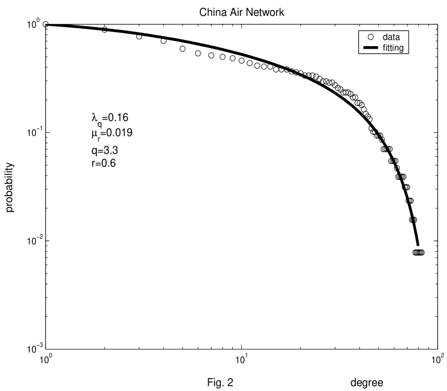
Figure 2: Degree distribution (points) of China air network. The line comes from the fitting using Eq. (7) where the four parameters $\mu_{r}$, $\lambda_{q}$, $q$ and $r$ were estimated directly from the data points.

As described in [20], the values of $\mu_{r}$, $\lambda_{q}$, $q$ and $r$ are first estimated directly from the curves depicted by the original data. Then using Eq. (7) and treating the observed values of $p(k)$ as inputs, the values of $k$ are fitted. The results are plotted in figure 2 to 4. The values of $q$ for the three networks are of same order as $q_{1}$’s from the separate fitting described above, while the values of $r$ are all 0.6 and very different from $q_{2}$’s. As in the separate fitting, the $q$ value for the composite network China+US is smaller than the $q$ value for China network and larger than the $q$ for US network. The fittings are globally fine, but with a small deviation observed at the “knee” between the two regimes: the theoretical curves do not have knees as distinct as the observed curves. The above fitting procedures as well as other techniques[22] we checked for fitting these two regime degree distributions will be described in details in another paper.

Although the above fittings are not perfect, we can say that Tsallis distribution function can, with the actually used mathematics, offer a satisfactory description of the observed laws. One of the consequences of these calculations is: systems obeying NS and composed of different $q$ subsystems all obeying NS exist. As a matter of fact, this existence is evident by a simple reasoning. Suppose there is a unique $q$ in the Universe, then it must be $q=1$ because we know there are systems in the Universe that obey BGS. This contradicts the starting hypothesis of the necessity of NS. Clearly, in general, Eq.(3) can not exist. In what follows, we propose an extension of it, the first one as far as we know.

3 An alternative nonadditivity rule of entropy

The aim of the following sections is to provide a possible formulation of NS which allows this kind of complicated system composition. For this purpose, PJP is abandoned as basic postulate. We take the entropy $S_{q}$ and the nonadditive rule of entropy as two basic hypothesis of the theory.

Now let us consider $A$ and $B$, two nonextensive subsystems of a composite nonextensive system $A+B$. It has been proved[6] that the most general pseudoadditivity (or composability) of entropy or energy prescribed by zeroth law is the following :

$$H[Q(A+B)]=H[Q(A)]+H[Q(B)]+\lambda_{Q}H[Q(A)]H[Q(B)],$$ (9)

which is in fact a very weak condition where $H[Q]$ is just certain differentiable function satisfying $H[0]=0$, $\lambda_{Q}$ is a constant, and $Q$ is either entropy $S$ or internal energy $U$[7]. As shown in [7], for a given relationship $Q=f(N)$ where $N$ is the (additive) number of elements of the system, the finding of $H(Q)$ is trivial. Eq.(9) has been established[6, 7] for the class of systems containing subsystems having same $q$. The generalization of it to the systems whose subsystems have different $q$’s is straightforward if we replace the Eq.(1) of reference [6], i.e., $S(A+B)=f\{S(A),S(B)\}$ for uniform $q$, by $H_{q}[S_{q}(A+B)]=f\{H_{q_{A}}[S_{q_{A}}(A)],H_{q_{B}}[S_{q_{B}}(B)]\}$ (or by $H_{q}[S_{q}(A+B)]=H_{q_{A}}[S_{q_{A}}(A)]+H_{q_{B}}[S_{q_{B}}(B)]+g\{H_{q_{A}}[S_{q_{A}}(A)],H_{q_{B}}[S_{q_{B}}(B)]\}$) where $H_{q}(S_{q})$ is a functional depending on $q$’s in the same way for the composite system as for the subsystems, where $q$, $q_{A}$ and $q_{B}$ are the parameters of the composite system $A+B$, the subsystems $A$ and $B$, respectively. The function $f$ (or $g$) is to be determined by the consideration of the zeroth law. Now repeating the mathematical treatments described in the references [6, 7], we find

$$H_{q}[Q(A+B)]=H_{q_{A}}[Q(A)]+H_{q_{B}}[Q(B)]+\lambda_{Q}H_{q_{A}}[Q(A)]H_{q_{B}}[Q(B)].$$ (10)

Eq.(9) turns out to be a special case of Eq.(10) for same $q$ systems. In view of the form of Tsallis entropy, a possible choice is $H_{q}(S_{q})=\sum_{i=1}^{w}p_{i}^{q}-1=(1-q)S_{q}$ in Eq.(10) as proposed in [3]. This implies :

$$(1-q)S_{q}(A+B) = (1-q_{A})S_{q_{A}}(A)+(1-q_{B})S_{q_{B}}(B)$$

$$+ \lambda_{S}(1-q_{A})(1-q_{B})S_{q_{A}}(A)S_{q_{B}}(B)$$

Note that Eq.(3) is not derived from Eq.(9) but only postulated as a possible pseudoadditivity of Tsallis entropy. As stated in reference [23], Unless the (probability) composition law is specified, the question whether an entropy is or is not extensive has no sense. Here we apply this reasoning inversely, i.e., we specify a nonadditivity rule of entropy and look for the corresponding probability composition rule. Let $\lambda_{S}=1$, Eq.(3) implies[3] :

$$p_{ij}^{q}(A+B)=p_{i}^{q_{A}}(A)p_{i}^{q_{B}}(B)$$ (12)

which can be called the extended factorization of joint probability for the systems of different $q$’s. Eq.(12) can be $formally$ written as the usual PJP $p_{ij}(A+B)=p_{i}(A)p_{j}(B)$ if and only if $q_{A}=q_{B}$. This extended PJP is nothing but the consequence of a kind of dependence of the subsystems. It is only one composition law of probability among many other possible ones corresponding to different additivity and nonadditivity of entropy, as indicated in [23]. The physical or effective probability is now $p_{i}^{q}$ instead of $p_{i}$. This interpretation may help to understand why $p_{i}^{q}$ or the escort probability $p_{i}^{q}/\sum_{i}p_{i}^{q}$[2] should be used for defining expectation in the same way for both the composite systems and the subsystems.

We would like to emphasize that Eq.(12) is only a result of the postulated nonadditivity rule Eq.(3). The proposition of this rule is in fact inspired by a study of nonequilibrium systems evolving in hierarchically heterogeneous phase space[24]. It has been shown that the above chosen functional form $H_{q}(S_{q})=\sum_{i=1}^{w}p_{i}^{q}-1$ is a measure of the variation of information (dynamical uncertainty) during the evolution if the normal rule $\sum_{i=1}^{w}p_{i}=1$ holds, and that $q$ is a ratio between the Hausdorff dimension and the topological dimension of the phase space if the latter is fractal. So the choice of Eq.(3) is relevant at least in this case where Tsallis formula can be used to measure entropy change in time.

4 Determination of the composite $q$

Eq.(12) allows one to determine uniquely the parameter $q$ for the composite system if $q_{A}$, $q_{B}$, $p_{i}(A)$ and $p_{j}(B)$ are given. By the normalization of the joint probability, we obtain the following relationship :

$$\sum_{i=1}^{w_{A}}p_{i}^{q_{A}/q}(A)\sum_{j=1}^{w_{B}}p_{j}^{q_{B}/q}(B)=1$$ (13)

which means $q_{A}<q<q_{B}$ if $q_{A}<q_{B}$ and $q=q_{A}=q_{B}$ if $q_{A}=q_{B}$. In this way, for a composite system containing $N$ subsystems (k=1,2,…,N) having different $q_{k}$, the parameter $q$ is determined by

$$\prod_{k=1}^{N}\sum_{i_{k}=1}^{w_{k}}p_{i_{k}}^{q_{k}/q}=1,$$ (14)

from which we can say that $mini(q_{k})<q<maxi(q_{k})$. In order to see more clearly the method, we suppose equiprobability for each subsystems, i.e., $p_{i_{k}}=(\frac{1}{w_{k}})^{1/q_{k}}$. In this case, we have

$$\prod_{k=1}^{N}\sum_{i_{k}=1}^{w_{k}}\left(\frac{1}{w_{k}}\right)^{q_{k}/q}=1,$$ (15)

which means

$$\prod_{k=1}^{N}\left(\frac{1}{w_{k}}\right)^{q_{k}}=\prod_{k=1}^{N}\left(\frac{1}{w_{k}}\right)^{q}$$ (16)

or

$$q=\sum_{k=1}^{N}q_{k}\ln{w_{k}}/\sum_{k=1}^{N}\ln{w_{k}}.$$ (17)

$q$ is a kind of barycenter of the sub $q$ values. If $w_{1}=w_{2}=...=w_{N}$, Eq.(17) becomes

$$q=\frac{1}{N}\sum_{k=1}^{N}q_{k}.$$ (18)

5 Temperature definition through zeroth law

A zeroth law for different $q$ systems has been briefly discussed in [3] with the help of a deformed entropy and energy. Following is a recapitulation of that method using directly the entropy $S_{q}$ and energy $U_{q}$. If $(A+B)$ is at equilibrium or stationary state optimizing Tsallis entropy $dS_{q}(A+B)=0$, considering Eq.(3), we get :

$$\frac{(1-q_{A})dS_{q_{A}}(A)}{1+(1-q_{A})S_{q_{A}}(A)}+\frac{(1-q_{B})dS_{q_{B}}(B)}{1+(1-q_{B})S_{q_{B}}(B)}=0$$ (19)

Notice the difference between this relation and $\frac{dS_{q}(A)}{1+(1-q)S_{q}(A)}+\frac{dS_{q}(B)}{1+(1-q)S_{q}(B)}=0$ which has been used for the systems of same $q$.

In order to find the suitable nonadditive rule of energy, we consider Eq.(12) and the relationship $\sum_{i}p_{i}^{q}=Z_{q}^{1-q}+(1-q)\beta U_{q}$ calculated from the distribution Eq.(2) and the unnormalized expectation $U_{q}$, we get

$$Z_{q}^{1-q}(A+B)+(1-q)\beta(A+B)U_{q}(A+B)$$ (20)

$$=[Z_{q_{A}}^{1-q_{A}}(A)+(1-q_{A})\beta(A)U_{q_{A}}(A)][Z_{q_{B}}^{1-q_{B}}(B)+(1-q_{B})\beta(B)U_{q_{B}}(B)].$$

Then the total energy conservation $dU_{q}(A+B)=0$ leads to

$$\frac{(1-q_{A})\beta(A)dU_{q_{A}}(A)}{\sum_{i}p_{i}^{q_{A}}(A)}+\frac{(1-q_{B})\beta(B)dU_{q_{B}}(B)}{\sum_{i}p_{i}^{q_{B}}(B)}=0$$ (21)

which suggests following energy nonadditivity

$$\frac{(1-q_{A})dU_{q_{A}}(A)}{\sum_{i}p_{i}^{q_{A}}(A)}+\frac{(1-q_{B})dU_{q_{B}}(B)}{\sum_{i}p_{i}^{q_{B}}(B)}=0$$ (22)

as the analog of the additive energy $dU(A)+dU(B)=0$ of BGS. From Eq.(22) and Eq.(19) follows

$$\frac{\partial S_{q_{A}}(A)}{\partial U_{q_{A}}(A)}=\frac{\partial S_{q_{B}}(B)}{\partial U_{q_{B}}(B)}$$ (23)

so the inverse temperature can be defined by $\beta=\frac{\partial S_{q}}{\partial U_{q}}$ for any system with whatever $q$.

We would like to emphasize here that Eq.(23) allows us to measure the temperature of a system with a thermometer having different $q$ values, as far as the system and the thermometer are in thermal equilibrium or local thermal equilibrium at the point of contact. This result mathematically supports a previous numerical work of [8, 17] showing the possibility to measure the temperature of a non Boltzmannian nonequilibrium system with a Boltzmannian thermometer.

It should be noticed that the present result is obtained with the unnormalized expectation of energy. In view of the important role of the escort probability in NS, an extension of NS to different $q$ system with the expectation defined with escort probability is indeed necessary. This possibility will be investigated in our future work on the basis of the extended PJP.

6 Concluding remarks

In the first part of this work, we fitted the power law degree distribution in two regimes of some airport networks with the $q$-exponential distribution of nonextensive statistics. The results prove with sufficient exactitude the existence of different $q$ subnetworks and composite networks all obeying $q$-exponential distribution. This situation requires formulation of NS allowing the composition of different $q$ systems. A crucial step is to show that temperature can be uniform in the nonextensive systems at equilibrium or local equilibrium states optimizing Tsallis entropy, independently of whether or not the systems contain subsystems with different $q$ values.

This formulation is constructed on the basis of an extended nonadditivity rule of entropy taken as a basic hypothesis of the theory. In this case, the conventional PJP is replaced by an extended PJP which signifies a kind of dependence between subsystems. Even when PJP is recovered in the special case of unique $q$, it has nothing to do with the independence of subsystems in the context of nonextensive and nonadditive systems. This is an idea expressed in a previous discussion [23]. As indicated above, this is only one of the possible formulations of NS with a pseudoadditivity rule. Further investigation is necessary to see the physics behind each possible composition law of entropy and probability.

We would like to mention here that the extended PJP and the usual normalization condition together prescribe two possible ways for generalizing NS to different $q$ systems: the first is with the unnormalized expectation as has be done in the present work; the second is with the normalized expectation given by the escort probability. These two definitions of expectation allow simple composition rules of expectation of physical quantities. The possibility of generalizing NS with the escort probability is actually under investigation.

Figure 1: Degree distributions (circles) of China airline network (top panel), US airline network (middle panel), and airline network of China plus US (bottom panel). The straight lines are fittings of the observed laws with the q-distribution given by Eq.(5). In order to show the deviation of the observed two regime distribution from exponential law, this latter is represented in the figure by curved lines.

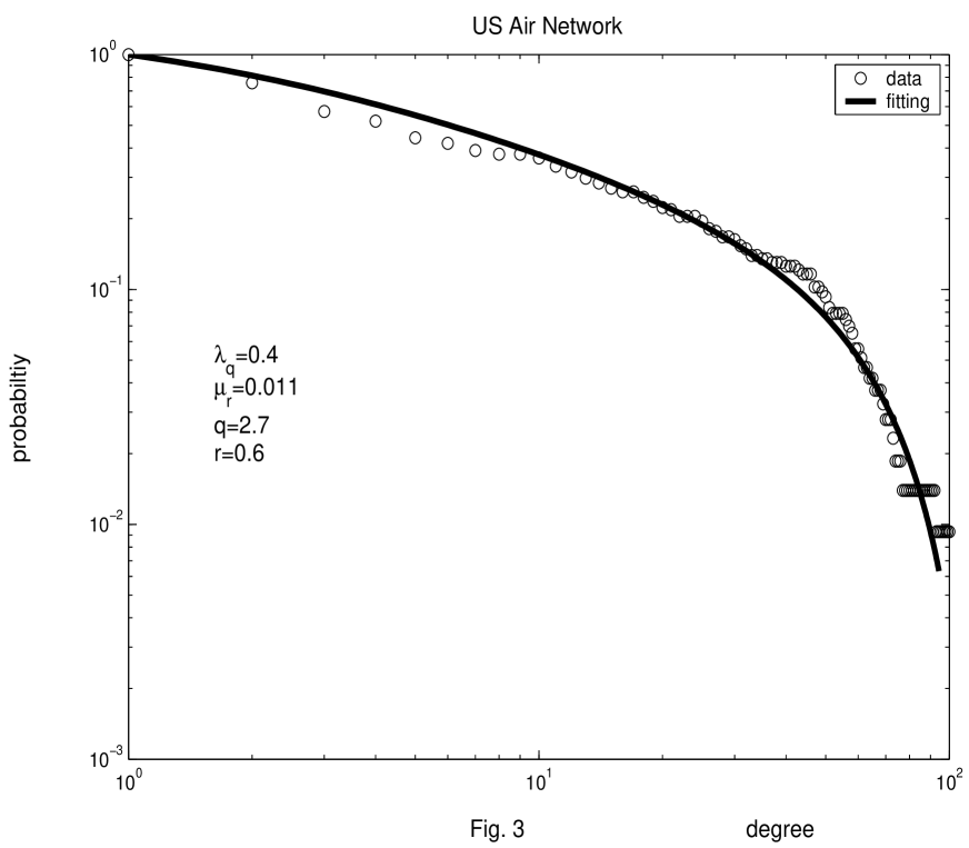
Figure 3: Degree distribution (points) of US air network. The line comes from the fitting using Eq. (7) where the four parameters $\mu_{r}$, $\lambda_{q}$, $q$ and $r$ were estimated directly from the data points.

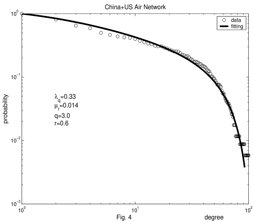
Figure 4: Degree distribution (points) of China+US air network. The line comes from the fitting using Eq. (7) where the four parameters $\mu_{r}$, $\lambda_{q}$, $q$ and $r$ were estimated directly from the data points.

References

- [1] C. Tsallis, J. Stat. Phys., 52,479(1988)
- [2] C. Tsallis, R.S. Mendes and A.R. Plastino, Physica A, 261,534(1999)
- [3] Q.A. Wang, L. Nivanen, A. Le Mehaute and M. Pezeril, Europhys. Lett., 65(2004)606
- [4] R. J. V. dos Santos, J. Math. Phys. 38 (1997) 4104;
- [5] S. Abe, Phys. Lett. A, 271,74(2000)
- [6] S. Abe, Phys. Rev. E, 63,061105(2001)
- [7] Q.A. Wang, L. Nivanen, A. Le Méhauté and M. Pezeril, J. Phys. A, 35,7003(2002)
- [8] C. Tsallis, Comment on ”A Critique of -entropy for thermal statistics” by M. Nauenberg, Phys. Rev. E, 69,038101(2004); cond-mat/0304696
- [9] K. Sasaki and M. Hotta, Chaos, Solitons Fractals, 13,513(2002)
- [10] M. Nauenberg, Phys. Rev. E, 67,036114(2002); Reply to C. Tsallis’ “Comment on critique of -entropy for thermal statistics by M. Nauenberg”, cond-mat/0305365v1
- [11] C. Beck, Physica A,277(2000)115
- [12] A.R. Plastino, A Plastino and Tsallis,J. Phys. A : Math. Gen.,27(1994)5707; C. Tsallis, News trends in magnetic materials and their applications, ed. J. L. Morán-López and J.M. Sánchez(New York, Plenum); A.R. Plastino and A. Plastino, Phys. Lett.A,174(1993)384
- [13] A. Lavagno, G. Kaniadakis, M. Rego-Monteiro, P. Quarati, and C. Tsallis, Astro. Lett. and Commun.,35(1998)449
- [14] G. Kaniadakis, A. Lavagno and P. Quarati, Phys. Lett.B,369(1993)308
- [15] D.J.B. Soares, C. Tsallis, A.M. Mariz and L.R. da Silva, cond-mat/0410459
- [16] A.L. Barabasi H. Jeong, Z. Neda, E. Ravasz, A. Schubert, T. Vicsek, Physica A, 311(2002)590
- [17] L.G. Moyano, F. Baldovin, C. Tsallis, Zeroth principle of thermodynamics in ageing quasistationary states, cond-mat/0305091
- [18] W. Li and X. Cai, Physical Review E 69, (2004)046106
- [19] L.P. Chi et al, Chin. Phys. Lett. 20 (No.8), (2003)1393
- [20] C. Tsallis, G. Bemski, and R.S. Mendes, Phys. Lett.A, 257, 93 (1999).
- [21] C. Tsallis, J.C. Anjos, and E.P. Borges, Phys. Lett.A,310(2003)372
- [22] Alain Le Méhauté, Annales du Centre de Recherche d’Urbanisme, (1974)141
- [23] C. Tsallis, Is the entropy S extensive or nonextensive? To appear in the Proceedings of the 31st Workshop of the Inter-national School of Solid State Physics Complexity, Metastability and Nonextensivity, held at the Ettore Majorana Foundation and Centre for Scientific Culture, Erice (Sicily) in 20-26 July 2004, eds. C. Beck, A. Rapisarda and C. Tsallis (World Scientific, Singapore, 2005); cond-mat/0410459
- [24] Q.A. Wang, Maximum entropy change and least action principle for nonequilibrium systems, Astrophysics and Space Science, (2005) in press; Q.A. Wang, A. Le M haut , L. Nivanen, M. Pezeril, Physica A, 340(2004)117