Probing Non-Abelian Statistics with Quasiparticle Interferometry

Abstract

We examine interferometric experiments in systems that exhibit non-Abelian braiding statistics, expressing outcomes in terms of the modular S-matrix. In particular, this result applies to FQH interferometry, and we give a detailed treatment of the Read-Rezayi states, providing explicit predictions for the recently observed $\nu=12/5$ plateau.

Quantum systems in two spatial dimensions allow for exotic exchange statistics, characterized by a unitary representation of the braid group Leinaas and Myrheim (1977); Wilczek (1982). This representation may be non-Abelian, acting on a multi-dimensional internal Hilbert space Goldin et al. (1985); Fröhlich (1988). So far, experimental evidence for the existence of such anyonic statistics has only recently been found in the (Abelian) Laughlin states of Fractional Quantum Hall (FQH) systems Camino et al. (2005a, b). However, the prospect of non-Abelian statistics is far more exciting, especially in light of its potential application in topologically fault-tolerant quantum computation Kitaev (2003); Freedman et al. (2002). There are currently several observed FQH states, at filling fractions $\nu=5/2,7/2,12/5$ Willett et al. (1987); Pan et al. (1999); Xia et al. (2004) (and possibly $\nu=3/8,19/8$), that are expected to possess non-Abelian statistics. Numerical studies Morf (1998); Rezayi and Haldane (2000); Read and Rezayi (1999) suggest that the $\nu=5/2,12/5$ states should be described respectively by the Moore-Read (MR) state Moore and Read (1991) and the $k=3,M=1$ Read-Rezayi (RR) state Read and Rezayi (1999). Clearly, as experimental capabilities progress, it becomes increasingly important to understand how to probe and correctly identify the braiding statistics of quasiparticles. In this Letter, we explain how, for any system described by a topological quantum field theory (TQFT) in the infrared limit (e.g. FQH systems), knowledge of modular S-matrices may be used to extract this information from interferometry experiments, or, inversely, to predict the outcomes of such experiments. As an example relevant to current experimental interests, we obtain explicit results for the RR states.

The topological properties of 2D quantum systems with an energy gap can be described using TQFTs (or “modular tensor categories” in mathematicians’ terminology, see e.g. Preskill (2004); Kitaev (2006); Turaev (1994); Kassel (1995)), often abstracted from conformal field theories (CFTs, see Di Francesco et al. (1997) and references therein). Such an anyon model is defined by (i) a finite set $\mathcal{C}$ of particle types or “anyonic charges,” (ii) fusion rules specifying how these particle types may combine or split, and (iii) braiding rules dictating the behavior under exchange of two particles (all subject to certain consistency conditions). The “vacuum” charge is given the label $\openone$. The anti-particle or “charge conjugate” of a particle type $a$ is denoted $\overline{a}$, and is the unique charge that can fuse with $a$ to give $\openone$. Fusion of particle types generalizes the addition of charges or angular momenta and the (commutative and associative) fusion rules are specified as $a\!\times b=\sum_{c\in\,\mathcal{C}}N_{ab}^{c}\,c$, where the integer $N_{ab}^{c}$ is the dimension of the Hilbert space of particles of type $a$ and $b$ restricted to have total anyonic charge $c$. Fusion and braiding can be represented diagrammatically on oriented, labeled particle worldlines, and are unaffected by smooth deformations in which the lines do not intersect. Charge conjugation is represented by reversal of wordline orientation. We will refer to only one braiding relation, known as the modular S-matrix, defined by the following diagram:

$$S_{ab}=\frac{1}{D}\pspicture[0.5](68.28658pt,36.98856pt){\psset{linewidth=1.0pt,linecolor=black,arrows=<-,arrowscale=1.5,arrowinset=0.15}\psarc{<-}(45.52438pt,19.91692pt){14.22636pt}{165.0}{363.0}}{\psset{linewidth=1.0pt,linecolor=black}\psarc(25.60747pt,19.91692pt){14.22636pt}{0.0}{180.0}}{\psset{linewidth=1.0pt,linecolor=black,border=3pt,arrows=->,arrowscale=1.5,arrowinset=0.15}\psarc{->}(25.60747pt,19.91692pt){14.22636pt}{180.0}{375.0}}{\psset{linewidth=1.0pt,linecolor=black,border=3pt}\psarc(45.52438pt,19.91692pt){14.22636pt}{0.0}{160.0}}{\psset{linewidth=1.0pt,linecolor=black}\psarc(45.52438pt,19.91692pt){14.22636pt}{155.0}{170.0}}\rput[bl]{0.0}(4.2679pt,8.53581pt){$a$}\rput[bl]{0.0}(61.17339pt,8.53581pt){$b$}\endpspicture.$$ (1)

Here $D=\sqrt{\sum\nolimits_{a}d_{a}^{2}}=1/S_{\openone\openone}$ is the total quantum dimension, where $d_{a}$, the quantum dimension of particle type $a$, is the value of a single loop of that type,

$$d_{a}=\pspicture[0.5](42.67911pt,36.98856pt){\psset{linewidth=1.0pt,linecolor=black,arrows=->,arrowscale=1.5,arrowinset=0.15}\psarc{->}(19.91692pt,19.91692pt){14.22636pt}{0.0}{373.0}}\rput[bl]{0.0}(35.56592pt,8.53581pt){$a$}\endpspicture=DS_{{\openone}a}\,.$$ (2)

Some useful properties of the S-matrix are

$$S_{ab}=S_{ba}=\overline{(S^{-1})}_{ab}=\overline{S}_{\overline{a}b}\,.$$ (3)

The importance of the S-matrix becomes clear when one envisions interferometry experiments for these systems in which a particle has two possible paths that it may take around another particle, the two paths combining to form a closed loop. This is typical of Mach-Zender, two-slit, FQH two-point-contact, etc. experiments Verlinde (1991); Lo and Preskill (1993); Bais et al. (1992, 1993); de C. Chamon et al. (1997); Fradkin et al. (1998); Overbosch and Bais (2001); Das Sarma et al. (2005); Stern and Halperin (2006); Bonderson et al. (2006). In such experiments, an interference term arises that can be written as

$$\left\langle\Psi_{ab}\right|U_{1}^{-1}U_{2}\left|\Psi_{ab}\right\rangle=e^{i\alpha_{ab}}\left\langle\Psi_{ab}\right|\mathbb{M}\left|\Psi_{ab}\right\rangle=e^{i\alpha_{ab}}M_{ab}$$ (4)

where $\left|\Psi_{ab}\right\rangle$ is the initial state of particles $a$ and $b$, and $U_{1},U_{2}$ are the unitary evolution operators for the particle $a$ traveling around the particle $b$ via the two respective paths. It has been rewritten in terms of the monodromy operator $\mathbb{M}$ that contains only the contribution from adiabatically transporting particle $a$ around particle $b$ (i.e. braiding), and a phase $e^{i\alpha_{ab}}$ that absorbs all other contributions (i.e. it contains the free particle dynamics and the Aharonov-Bohm phase from a background magnetic flux). For simplicity, we let the two particles have definite anyonic charge, however it is a straightforward generalization to allow superpositions of particle type. If the theory only has Abelian statistics, then $\left|M_{ab}\right|=1$, but with non-Abelian statistics, $\left|M_{ab}\right|$ can be less than $1$ and must be calculated by TQFT methods. The braiding term is diagrammatically represented by winding the worldline of particle $a$ around that of particle $b$, taking the standard closure (where the worldline of each particle is closed back on itself in a manner that introduces no additional braiding) and dividing by the quantum dimension of the two particle types . Thus, the resulting monodromy matrix element can be written entirely in terms of the S-matrix:

$$M_{ab}=\frac{1}{d_{a}d_{b}}\pspicture[0.5](68.28658pt,36.98856pt){\psset{linewidth=1.0pt,linecolor=black,arrows=<-,arrowscale=1.5,arrowinset=0.15}\psarc{<-}(45.52438pt,19.91692pt){14.22636pt}{165.0}{363.0}}{\psset{linewidth=1.0pt,linecolor=black}\psarc(25.60747pt,19.91692pt){14.22636pt}{0.0}{180.0}}{\psset{linewidth=1.0pt,linecolor=black,border=3pt,arrows=->,arrowscale=1.5,arrowinset=0.15}\psarc{->}(25.60747pt,19.91692pt){14.22636pt}{180.0}{375.0}}{\psset{linewidth=1.0pt,linecolor=black,border=3pt}\psarc(45.52438pt,19.91692pt){14.22636pt}{0.0}{160.0}}{\psset{linewidth=1.0pt,linecolor=black}\psarc(45.52438pt,19.91692pt){14.22636pt}{155.0}{170.0}}\rput[bl]{0.0}(4.2679pt,8.53581pt){$a$}\rput[bl]{0.0}(61.17339pt,8.53581pt){$b$}\endpspicture=\frac{S_{ab}S_{\openone\openone}}{S_{{\openone}a}S_{{\openone}b}}\,.$$ (5)

This result is particularly nice because the S-matrix is typically more readily computable than the complete set of braiding/fusion rules, and, in fact, has already been computed for most physically relevant theories. In particular, this applies to the class of theories described by CFTs generated as products and cosets of Wess-Zumino-Witten theories, which includes all proposed non-Abelian FQH states (see Fröhlich et al. (2001); Wen (1991); Ardonne and Schoutens (1999); Ardonne et al. (2002)). In the case of the product of two CFTs or TQFTs, the particle types are denoted by pairs of particle labels, one from each theory, and the S-matrix of the product theory is the tensor product of the S-matrices of the parent theories. In the ${G}_{k}/{H}_{l}$ coset theory, the new labels are also formed as pairs of labels from the parent ${G}_{k}$ and ${H}_{l}$ theories, but now there are branching rules which restrict the allowed pairings. Also, different pairs of labels may sometimes turn out to represent the same particle type, a phenomenon described by “field identifications”. This means that there will be only one row and column in the S-matrix for any set of identified labels. Despite these complications, the coset’s S-matrix elements are described by the simple formula Gepner (1989)

$$S^{(G/H)}_{(a,p)(b,q)}=c(G,H,k,l)\,S^{(G)}_{ab}\bar{S}^{(H)}_{pq}$$ (6)

where $a,b$ and $p,q$ are respectively labels of the ${G}_{k}$ and ${H}_{l}$ theories, and $c(G,H,k,l)$ is an overall normalization constant that enforces unitarity of the S-matrix (but is irrelevant in Eq. (5)).

We now focus specifically on FQH systems, because they are the only physical systems found to exhibit braid statistics thus far, and represent the most likely candidates for finding non-Abelian statistics. We consider the interferometry experiment originally proposed in de C. Chamon et al. (1997) for measuring braiding statistics in the Abelian FQH states, which was later adopted for the non-Abelian case in Fradkin et al. (1998) and addressed again in the context of the $\nu=5/2$ state in Stern and Halperin (2006); Bonderson et al. (2006). A somewhat similar experiment has recently been implemented to probe the Abelian $\nu=1/3$ state Camino et al. (2005a, b). The experimental setup is a two point-contact interferometer composed of a quantum Hall bar with two front gates on either side of an antidot (see Fig. 1). Biasing the front gates, one may create constrictions in the Hall bar, adjusting the tunneling amplitudes $t_{1}$ and $t_{2}$. Tunneling between the opposite edge currents leads to a deviation of $\sigma_{xy}$ from its quantized value, or equivalently, to the appearance of $\sigma_{xx}$. By measuring $\sigma_{xx}$ one effectively measures the interference between the two tunneling paths around the antidot. The tunneling amplitudes $t_{1}$ and $t_{2}$ must be kept small, to ensure that the tunneling current is completely due to quasiholes rather than higher charge composites , and to allow us to restrict our attention to the lowest order winding term.

In order to be able to influence the resulting interference pattern, we envision several experimentally variable parameters: (i) the central gate voltage allowing one to control the number $n$ of quasiholes on the antidot, (ii) the perpendicular magnetic field $B$, (iii) the back gate voltage controlling the uniform electron density, and (iv) the side gate that can be used to modify the shape of the edge inside the interferometric loop Stern and Halperin (2006). The intention is to be able to separately affect the Abelian Aharonov-Bohm phase and the number of quasiholes on the antidot; from this point of view having all these controls is redundant, but may be found beneficial for experimental success.

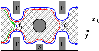
Figure 1: A two point-contact interferometer for measuring braiding statistics. The hatched region contains an incompressible FQH liquid. The front gates (F) are used to bring the opposite edge currents (indicated by arrows) close to each other to form two tunneling junctions. Applying voltage to the central gate creates an antidot in the middle and controls the number $n$ of quasiholes contained there. An additional side gate (S) can be used to change the shape and the length of one of the paths in the interferometer.

The longitudinal conductivity is proportional to the probability that current entering the bottom edge will leave through the top edge, which to lowest order is:

$$\sigma_{xx} \propto \left|t_{1}\right|^{2}+\left|t_{2}\right|^{2}+2\text{Re}\left\{t_{1}^{\ast}t_{2}\left\langle\Psi_{ab}\right|U_{1}^{-1}U_{2}\left|\Psi_{ab}\right\rangle\right\}$$ (7)

$$= \left|t_{1}\right|^{2}+\left|t_{2}\right|^{2}+2\left|t_{1}t_{2}\right|\left|M_{ab}\right|\cos\left(\beta+\theta_{ab}\right)\,.$$

In this equation $\beta=\alpha_{ab}+\arg\left(t_{2}/t_{1}\right)$ can be varied by changing B (keeping the quasihole number fixed), the relative tunneling phase, and/or the edge shape around the central region. We have written $M_{ab}=\left|M_{ab}\right|e^{i\theta_{ab}}$, and will be interested in the elements where the particle $a$ which tunnels carries the anyonic charge of a quasihole, while the “particle” $b$ is a composite of $n$ quasiholes on the antidot, carrying an anyonic charge allowed by the fusion rules .

We will now apply this formalism to the RR states and, in particular, look more closely at the $k=3,M=1$ case, which, by a particle-hole transformation (which generally inverts the statistics and has the effect of conjugating the S-matrix), is the expected description of $\nu=12/5$. The anyon theory for RR states at $\nu=k/(kM+2)$ can be described as $\text{RR}_{k,M}=\text{U}(1)_{k,M}\times\text{Pf}_{k}$ where $\text{U}(1)_{k,M}$ is due to the electric charge and $\text{Pf}_{k}$ represents the $\mathbb{Z}_{k}$-parafermion theory Zamolodchikov and Fateev (1985); Gepner and Qiu (1987). The $\text{U}(1)_{k,M}$ part of this theory is a simple Abelian contribution, essentially labeled by integral multiples of the charge/flux unit $\left(\frac{e}{kM+2},\frac{2\pi}{ke}\right)$, where $-e$ is the electron charge and $\frac{2\pi}{e}=\Phi_{0}$ is the magnetic flux quantum (in units $\hbar=c=1$). The fusion rules for these labels are just addition of charge/flux and the S-matrix is $S_{n_{a}n_{b}}=e^{in_{a}n_{b}\frac{2\pi}{k\left(kM+2\right)}}/\sqrt{k(kM+2)}$.

The $\text{Pf}_{k}$ part of this theory requires more explanation (for a discussion of its braiding, see Slingerland and Bais (2001)). Essentially, we use that the theory is equivalent to the coset ${\text{SU}(2)}_{k}/{\text{U}(1)}_{k}$. As a consequence, the $\mathbb{Z}_{k}$-parafermion sector’s anyonic charge can be labeled by the corresponding CFT fields $\Phi_{\lambda}^{\Lambda}$, where $\Lambda\in\left\{0,1,\ldots,k\right\}$ and $\lambda\in\mathbb{Z}$, subject to the identifications $\Phi_{\lambda}^{\Lambda}=\Phi_{\lambda+2k}^{\Lambda}=\Phi_{\lambda-k}^{k-\Lambda}$ and the restriction $\Lambda+\lambda\equiv 0\left(\text{mod}2\right)$ (giving a total of $\frac{1}{2}k\left(k+1\right)$ fields). The fusion rules for this sector are (as for the CFT fields):

$$\Phi_{\lambda_{a}}^{\Lambda_{a}}\times\Phi_{\lambda_{b}}^{\Lambda_{b}}=\sum\limits_{\Lambda=\left|\Lambda_{a}-\Lambda_{b}\right|}^{\min\left\{\Lambda_{a}+\Lambda_{b},2k-\Lambda_{a}-\Lambda_{b}\right\}}\Phi_{\lambda_{a}+\lambda_{b}}^{\Lambda}\,.$$ (8)

Their quantum dimensions are

$$d_{\Phi_{\lambda}^{\Lambda}}=\sin\left(\frac{\left(\Lambda+1\right)\pi}{k+2}\right)\mbox{\LARGE$/$}\sin\left(\frac{\pi}{k+2}\right)\,.$$ (9)

Special fields in this theory are the vacuum ${\openone}\equiv\Phi_{0}^{0}$, the $\mathbb{Z}_{k}$-parafermions $\psi_{l}\equiv\Phi_{2l}^{0}$, the primary fields $\sigma_{l}\equiv\Phi_{l}^{l}$, and the $\mathbb{Z}_{k}$-neutral excitations $\varepsilon_{j}\equiv\Phi_{0}^{2j}$, where $l=1,\ldots,k-1$ and $j=1,\ldots,\left\lfloor\left(k-1\right)/2\right\rfloor$. From (6) we find that the S-matrix for $\text{Pf}_{k}$ is

$$S_{\Phi_{\lambda_{a}}^{\Lambda_{a}}\Phi_{\lambda_{b}}^{\Lambda_{b}}}=\frac{\sin\left(\frac{\left(\Lambda_{a}+1\right)\left(\Lambda_{b}+1\right)\pi}{k+2}\right)}{D\sin\left(\frac{\pi}{k+2}\right)}e^{-i\lambda_{a}\lambda_{b}\pi/k}.$$ (10)

The $\text{U}(1)_{k,M}$ and $\text{Pf}_{k}$ sectors combine so that the anyonic charges in the $\text{RR}_{k,M}$ theory are (defining a shorthand) $\hat{\Lambda}_{n}\!\!\!\!\equiv\!\!\!\!\left(\frac{ne}{kM+2},\frac{n2\pi}{ke},\Phi_{n}^{\Lambda_{n}}\right)$, where we have $n\!\!\!\!\in\!\!\!\!\mathbb{Z}$ and $\Lambda_{n}\in\left\{0,1,\ldots,k\right\}$ such that $\Lambda_{n}+n\equiv 0\left(\text{mod}2\right)$. Quasiholes carry charge $\hat{1}_{1}=\left(\frac{e}{kM+2},\frac{2\pi}{ke},\sigma_{1}\right)$. The S-matrix for RR anyons is obtained by multiplying the S-matrix elements of the two sectors for anyons $a$ and $b$, and renormalizing by some overall constant $c$ (which we will not need explicitly):

$$S_{ab}=c\sin\left(\frac{\left(\Lambda_{n_{a}}+1\right)\left(\Lambda_{n_{b}}+1\right)\pi}{k+2}\right)e^{-in_{a}n_{b}\frac{M\pi}{kM+2}}.$$ (11)

Since the tunneling current is dominated by quasiholes , we only need the monodromy matrix elements

$$M_{\hat{1}_{1},\hat{\Lambda}_{n}}\!\!=\frac{\cos\left(\frac{\left(\Lambda_{n}+1\right)\pi}{k+2}\right)}{\cos\left(\frac{\pi}{k+2}\right)}e^{-in\frac{M\pi}{kM+2}}.$$ (12)

We note that RR_2,1 is the MR state, and we can easily check that this exactly matches the results of Fradkin et al. (1998); Bonderson et al. (2006).

We now turn to the $\text{RR}_{3,1}$ theory for $\nu=12/5$. The $\text{Pf}_{3}$ theory has six fields: $\openone$, $\psi_{1}$, $\psi_{2}$, which have quantum dimension $1$, and $\sigma_{1}$, $\sigma_{2}$, $\varepsilon$, which have quantum dimension $\phi=2\cos\frac{\pi}{5}=\frac{1+\sqrt{5}}{2}$ (the golden ratio). The total quantum dimension is $D=\sqrt{3\left(\phi+2\right)}$ and the S-matrix is

$$S=\frac{1}{D}\left[\begin{array}[]{cccccc}1&1&1&\phi&\phi&\phi\\ 1&e^{i\frac{2\pi}{3}}&e^{-i\frac{2\pi}{3}}&\phi e^{-i\frac{2\pi}{3}}&\phi e^{i\frac{2\pi}{3}}&\phi\\ 1&e^{-i\frac{2\pi}{3}}&e^{i\frac{2\pi}{3}}&\phi e^{i\frac{2\pi}{3}}&\phi e^{-i\frac{2\pi}{3}}&\phi\\ \phi&\phi e^{-i\frac{2\pi}{3}}&\phi e^{i\frac{2\pi}{3}}&e^{-i\frac{\pi}{3}}&e^{i\frac{\pi}{3}}&-1\\ \phi&\phi e^{i\frac{2\pi}{3}}&\phi e^{-i\frac{2\pi}{3}}&e^{i\frac{\pi}{3}}&e^{-i\frac{\pi}{3}}&-1\\ \phi&\phi&\phi&-1&-1&-1\end{array}\right]$$

where the columns and rows are in the order: $\openone$, $\psi_{1}$, $\psi_{2}$, $\sigma_{1}$, $\sigma_{2}$, $\varepsilon$. Quasiholes in the RR_3,1 theory have anyonic charge $\left(\frac{e}{5},\frac{2\pi}{3e},\sigma_{1}\right)$. It is useful to consider a Bratteli diagram (which has periodicity 6 in $n$) to keep track of the allowed $\text{Pf}_{3}$ charge for a corresponding value of $n$:

$$\begin{array}[]{ccccccccc}&3&\vrule\lx@intercol\hfil\lx@intercol&\psi_{2}&&\openone&&\psi_{1}&\\ &2&\vrule\lx@intercol\hskip 5.69054pt\varepsilon\hfil\lx@intercol&&\sigma_{2}&&\sigma_{1}&&\varepsilon\\ \Lambda_{n}&1&\vrule\lx@intercol\hfil\lx@intercol&\sigma_{1}&&\varepsilon&&\sigma_{2}&\\ &0&\vrule\lx@intercol\hskip 5.69054pt\openone\hfil\lx@intercol&&\psi_{1}&&\psi_{2}&&\openone\\[4.0pt] \cline{2-9}\cr&&\lx@intercol\hfil\lx@intercol&&&&&&\\[-8.53581pt] &n\rightarrow&\hskip 5.69054pt0&1&2&3&4&5&6\\ \end{array}$$

The longitudinal conductivity in the interferometry experiment will be

$$\sigma_{xx}\propto\left|t_{1}\right|^{2}\!+\left|t_{2}\right|^{2}\!+2\left|t_{1}t_{2}\right|\left(-\phi^{-2}\right)^{N_{\phi}}\!\cos\!\left(\beta+n\frac{4\pi}{5}\right)$$ (13)

where $N_{\phi}=1$ if the $n$ quasihole composite on the antidot has Pf₃ charge with quantum dimension $\phi$ (i.e. $\sigma_{1}$, $\sigma_{2}$, or $\varepsilon$) and $N_{\phi}=0$ if the composite has quantum dimension $1$ (i.e. $\openone$, $\psi_{1}$, or $\psi_{2}$). Thus, depending on the total Pf₃ charge on the antidot, one of two possible conductivity values will be observed. The Pf₃ charge may then be determined by varying $\beta$ (using the side gate) to measure the interference fringe amplitude, which is suppressed by a factor of $\phi^{-2}\approx.38$ when $N_{\phi}=1$. This behavior indicates the presence of non-Abelian statistics, and distinguishes this state from other proposals for the same filling fraction (e.g. composite fermions). To describe $\nu=12/5$, we apply a particle-hole transformation to $RR_{3,1}$, replacing $S$ with $\overline{S}$ (hence, $M$ with $\overline{M}$), which changes the sign in front of $n$ in Eq. (13) . In more general scenarios where composites of quasiholes/quasielectrons may be used instead of the single tunneling quasiholes, identical behavior (up to the phase) will be exhibited by quantum dimension $\phi$ composites, while quantum dimension $1$ composites exhibit a single unsuppressed interference pattern at any $n$.

We conclude with a few remarks explaining that despite the relatively simple nature of these interferometry experiments, they provide a surprisingly large amount of information about the system being probed. This is because the experiments essentially measure the S-matrix of the TQFT that describes the system. The S-matrix fully determines the fusion rules through the Verlinde formula Verlinde (1988): $N_{ab}^{c}=\sum_{x\in\,\mathcal{C}}S_{ax}S_{bx}S_{\overline{c}x}/S_{{\openone}x}$. Additionally, a theorem known as “Ocneanu rigidity” states that, given a set of fusion rules, there are only finitely many corresponding TQFTs with these rules Etingof et al. (2005). In other words, knowledge of the S-matrix is sufficient to pin down the topological order of the state to a finite number of possibilities. Clearly, it may be difficult to measure all elements of the S-matrix by the methods described here. It appears particularly challenging to invoke tunneling of anyonic charges different from that of the quasihole, though one may speculate on techniques that may eventually prove successful, such as resonant effects with intermediate antidots of tunable geometry and capacity on the tunneling arms. Still, the S-matrix has many special properties and so even a partial measurement of fairly low accuracy may be sufficient to determine it. In addition to Eq. (3), any S-matrix must satisfy a set of constraints coming from the Verlinde formula and the fact that the fusion coefficients are integers. Also, the first row of the S-matrix must be real and positive, because of its relation to the quantum dimensions (and in fact, all elements are numbers with special algebraic properties). Finally, given an S-matrix, there must be a diagonal matrix $T$ which together with $S$ generates a representation of the modular group $\text{SL}(2,\mathbb{Z})$, implying that $(ST)^{3}=S^{2}$. For any fixed number of particle types, only finitely many different S-matrices are known (and it is conjectured that only finitely many exist). Hence, once some the S-matrix elements and the number of different charges are known from measurements, one may look at the finite list of known S-matrices and hope to identify one that matches. In conclusion, for any two-dimensional system, interference experiments as described here can in principle determine the fusion rules and even a finite set of TQFTs, one of which will fully describe the topological order.