Renormalization group calculation of the uniform susceptibilities in low-dimensional systems

Abstract

We analyze the one-dimensional (1D) and the two-dimensional (2D) repulsive Hubbard models (HM) for densities slightly away from half-filling through the behavior of two central quantities of a system: the uniform charge and spin susceptibilities. We point out that a consistent renormalization group treatment of them can only be achieved within a two-loop approach or beyond. In the 1D HM, we show that this scheme reproduces correctly the metallic behavior given by the well-known Luttinger liquid fixed-point result. Then, we use the same approach to deal with the more complicated 2D HM. In this case, we are able to show that both uniform susceptibilities become suppressed for moderate interaction parameters as one take the system towards the Fermi surface. Therefore, this result adds further support to the interpretation that those systems are in fact insulating spin liquids. Later, we perform the same calculations in 2D using the conventional random phase approximation, and establish clearly a comparison between the two schemes.

1 Introduction

The anomalous electronic properties of the metallic phase of the copper-oxide high-Tc superconductors are widely believed to be linked to the manifestation of a non-Fermi liquid state arising from the two-dimensional (2D) character of those compounds. Motivated by this, physicists have then been trying to understand theoretically what are the precise conditions in which Landau’s Fermi liquid paradigm [1, 2] (i.e. the scheme based on the concept of low-lying electronic quasiparticles in the system) breaks down in 2D models.

There are a number of approaches for accomplishing that task in 2D systems. The most direct route is through Landau’s theory of spontaneous breaking of a continuous symmetry, often induced by an instability with respect to a relevant external perturbation. That case usually leads to a phase transition scenario accompanied by the realization of a long-range ordered state in the system. Moreover, it implies the onset of gapless low-energy elementary excitations: the so-called Goldstone modes (see Goldstone’s theorem in Refs. [3, 4]). This theory provides the framework for understanding, among several other examples, the long-range magnetic order realized in the Mott insulating state of the 2D Hubbard model (HM) exactly at half-filling, and the resulting emergence of gapless antiferromagnetic magnon excitations, which manifest themselves solely through the spontaneous breaking of the spin rotation symmetry in the system.

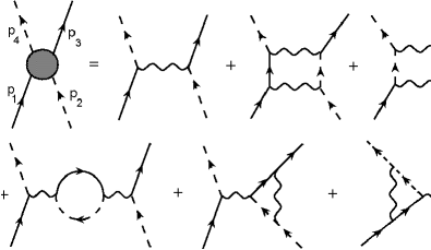
Figure 1: The Feynman diagrams for the one-particle irreducible four-point function $\Gamma^{(4)}(p_{1},p_{2},p_{3},p_{4})$ in the backscattering channel up to two-loop order (third order). The free propagators are represented by either solid or dashed lines according to their association with the corresponding branches.

Alternatively, another viable approach for that is produced quantum-mechanically by the disordering induced by strong fluctuations resulting from low-dimensionality effects themselves or by frustration effects in 2D models. These interacting regimes in turn do not have any broken symmetry realized in the ground state and, as a result, all the correlations are purely short-ranged in real space. In view of this, in principle, there can be no gapless excitations in those cases, since Goldstone’s theorem does not apply anymore. These exotic states cannot be described by the conventional Landau’s theory mentioned before, and are commonly referred to as spin liquid ground states. Their existence was first predicted by Anderson long ago in the context of a Heisenberg model defined on a 2D triangular lattice [5], and in [6] a decade later, and they might possibly hold the key for the appropriate theoretical explanation of the underlying mechanism of the high-Tc superconductors.

To understand these issues better, theorists have been generally looking for similar physics in simpler models. For instance, in strictly one-dimensional (1D) systems, the situation is far more understood in that respect [7, 8, 9]. It is by now very well-established that Landau’s Fermi liquid description breaks down completely in those particular cases. In fact, the appropriate effective low-energy theory for the 1D metallic state is instead the so-called Luttinger liquid. This happens due to specific features associated with 1D, i.e, the always nested Fermi surface (FS) consisting of only two discrete points ($+k_{F}$ and $-k_{F}$), and the very restricted phase space available for the elementary excitations above the corresponding ground state. Consequently, the low-energy excitation spectrum becomes fundamentally dominated by bosonic collective excitations given by two types: the holons and the spinons excitations. These particles in turn imply an exact separation of the charge and spin degrees of freedom in the system. As a result, they are most effective in destroying completely the fundamental picture of well-defined low-lying quasiparticles, which are the basis of Fermi liquid theory.

In this paper, it is our main goal to investigate the low-energy properties of the well-known 2D repulsive HM for densities slightly away from half-filling. To do this, we analyze two central quantities of the model: the uniform charge and spin susceptibilities. We choose these two physical quantities in view of the fact that they naturally provide important information about the existence or not of low-lying excitations in the system. As will become clear soon, to perform a full renormalization group (RG) calculation of those quantities, it is essential to set up at least a two-loop order RG calculation for it. As a testing ground of this approach, we first calculate these quantities in the 1D repulsive HM away from half-filling. In this case, we show that both quantities approach finite values, and the resulting low-energy description is indeed a metallic phase (in fact a Luttinger liquid) in agreement with well-known exact results (Bethe ansatz, bosonization, etc). Later, we apply the same considerations to the more complicated 2D HM, which is the case we are mainly interested here. We point out that there is an interaction regime, where both quantities become strongly suppressed as one approaches the low-energy limit, thus adding further support to the interpretation that the resulting effective theory should be given by an insulating spin liquid state [10]. Then, we compare these results with the conventional random phase approximation (RPA) case, and show that this latter approximation is not able to detect clearly such an exotic ground state in the system. Finally, we discuss the physical origins of the discrepancies of those two results.

2 Testing ground: The 1D repulsive Hubbard model

First of all, we define the Hubbard model (HM) defined on an 1D lattice here. This model describes a system of tight-binding electrons hopping only to nearest neighbor sites, and interacting mutually through a local (in real space) repulsive interaction parametrized by $U>0$. The corresponding Hamiltonian given in momentum space is

$$H=\sum_{k,\sigma}\xi_{k}\psi^{\dagger}_{k\sigma}\psi_{k\sigma}+\left(\frac{U}{N_{sites}}\right)\sum_{p,k,q}\psi^{\dagger}_{p+k-q\uparrow}\psi^{\dagger}_{q\downarrow}\psi_{k\downarrow}\psi_{p\uparrow},$$ (1)

where the single-particle energy dispersion is simply $\xi_{k}=-2t\cos ka-\mu$, and $\psi^{\dagger}_{k\sigma}$ and $\psi_{k\sigma}$ are the usual creation and annihilation operators of electrons with momentum $k$ and spin projection ${\sigma}=\uparrow,\downarrow$. Besides, $\mu$ stands for the chemical potential, $a$ is the lattice spacing, and $N_{sites}$ is the total number of lattice sites. Another important parameter here is the width of the noninteracting band, which is given by $W=4t$.

The FS of the noninteracting system is given by two discrete points ($+k_{F}$ and $-k_{F}$). Since we are mostly interested in the low-energy properties of this model, we linearize the energy dispersion about the two Fermi points, i.e., $\xi_{k}=v_{F}\left(\left|k\right|-k_{F}\right)$, where $v_{F}=(\partial\xi_{k}/\partial k)|_{k=k_{F}}$ is the Fermi velocity of the system. We restrict the allowed single-particle states to lie within the interval $k_{F}-\lambda\leq\left|k\right|\leq k_{F}+\lambda$, where $\lambda$ is a fixed ultraviolet (UV) microscopic momentum cut-off, and $\Omega$ is the corresponding energy cutoff given by $\Omega=2v_{F}\lambda$. As a result, we are able to identify two different regions in k-space: the “+” branch linearized about $k=+k_{F}$, and the “–” branch linearized about $k=-k_{F}$. Thus, the corresponding free propagators may be represented by two different lines in the Feynman diagrams: solid line for the former, and dashed line for the latter. In addition, regarding the interaction term, we use the standard g-ology parametrization [7], namely, the interaction processes involving large momentum transfers (near $2k_{F}$) are described by the $g_{1}$ coupling, whereas the processes involving small momentum transfers between particles located at different branches are described by the $g_{2}$ coupling. The former interactions are usually called backscattering processes, while the latter are referred to as forward scattering processes. In what follows, we will deliberately neglect the contributions due to the so-called Umklapp processes, which are described by the coupling $g_{3}$, in view of the fact that we will not consider here the exceptional case of an exact half-filled band in the model. Moreover, we will make one further approximation and neglect forward scattering pocesses between particles belonging to the same branch, which are conventionally described by the coupling constant $g_{4}$.

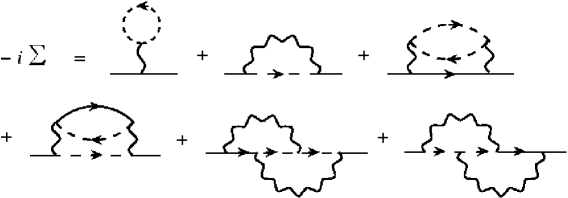
Figure 2: The self-energy diagrams up to two-loop order. The one-loop order (first order) diagrams are the nonsingular Hartree-Fock terms. The first nonanalyticity comes from the two-loop order (second order) diagrams.

In the following, we will use the so-called field-theoretical RG strategy to tackle this problem. In view of this, it is more convenient to work here with the Lagrangian of the model instead of the Hamiltonian. Thus, we write down the Lagrangian of the 1D HM as

$$L=\sum_{k,\sigma,a=\pm}\psi_{(a)\sigma}^{\dagger}\left(k,t\right)\left[i\partial_{t}-v_{F}\left(\left|k\right|-k_{F}\right)\right]\psi_{(a)\sigma}\left(k,t\right)$$

$$-\frac{1}{V}\sum_{p,q,k}\sum_{\alpha,\beta,\delta,\gamma}\left[g_{2}\delta_{\alpha\delta}\delta_{\beta\gamma}-g_{1}\delta_{\alpha\gamma}\delta_{\beta\delta}\right]\psi_{\left(+\right)\delta}^{\dagger}\left(p+q-k,t\right)\psi_{\left(-\right)\gamma}^{\dagger}\left(k,t\right)\psi_{\left(-\right)\beta}\left(q,t\right)\psi_{\left(+\right)\alpha}\left(p,t\right),$$

(2)

where $\psi^{\dagger}_{(\pm)}$ and $\psi_{(\pm)}$ are now fermionic fields associated to electrons located at the $\pm$ branches. The summation over momenta must be appropriately understood as $\sum_{p}=V/(2\pi)\int dp$ in the thermodynamic limit, where $V$ is the “volume” of the 1D system. Since this should represent the 1D HM, the Lagrangian is written in a manifestly $SU(2)$ invariant form and, in addition to this, the couplings are initially defined as $g_{1}=g_{2}=(V/4N_{sites})U$.

Since the HM is microscopic, the couplings and the fermionic fields in the Lagrangian are defined at a scale of a few lattice spacings in real space (i.e at the UV cutoff scale in momentum space). These parameters are usually inaccessible to every day experiments, since the latter probe only the low-energy dynamics of the system. In RG theory, these unobserved quantities are known as the bare parameters. In fact, when one tries to construct naive perturbative calculations with such quantities, one is immediately confronted with several Feynman diagrams, which turn out to be singular in the low-energy limit. These are the so-called infrared (IR) divergences in field theory. They appear in both backscattering and forward scattering four-point vertex corrections (see, for instance, Fig. 1), and in the calculation of the self-energy alike (Fig. 2). Those divergences do not imply necessarily that perturbation theory is simply unable to give any reliable prediction of the low-energy properties of the model, but only that the way it is formulated is not the appropriate one for this case. Therefore, one must generalize the perturbative approach so as to eliminate such singularities in the calculations. This is the strategy of the so-called renormalized perturbation theory, i.e, one rewrites all unobserved bare parameters in terms of the associated renormalized (or observable) quantities. The difference between them will be given by the so-called counterterms, whose essential role is to absorb all divergences up to a given order in perturbation theory. If this program is successfully accomplished, then the theory is said to be properly renormalized.

Following this, we have

$$\psi_{(a)\sigma} \rightarrow\psi_{(a)\sigma}^{R}+\Delta\psi_{(a)\sigma}^{R}=Z^{1/2}\psi_{(a)\sigma}^{R},$$ (3)

$$g_{i} \rightarrow Z^{-2}\left(g_{iR}+\Delta g_{iR}\right),\hskip 14.22636pt(i=1,2),$$ (4)

where $\psi_{(a)\sigma}^{R}$ and $g_{iR}$ are, respectively, the renormalized fields and couplings, whereas $\Delta\psi_{(a)\sigma}^{R}$ and $\Delta g_{iR}$ are the corresponding counterterms. Besides, $Z$ is the quasiparticle weight and measures the coherence of the quasiparticle picture in the effective (renormalized) description. As we explained in our previous paper [11], this parameter is related to the self-energy effects, and as such is essential for a consistent two-loop renormalization group analysis of the model.

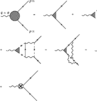
Figure 3: The Feynman diagrams for the uniform response function $\Gamma^{(2,1)}(p,q\approx 0)$ up to two-loop order. The triangular vertices stand for the renormalized response function, whereas the diagram with a cross represents the counterterm.

Nevertheless, there are still many ways to define the appropriate counterterms using the above prescription. In order to solve this ambiguity, we must establish a renormalization condition for the observable parameters. We use here the one-particle irreducible four-point and two-point functions (for standard definitions see, for instance, Ref. [12]). Therefore, we have

$$\Gamma^{(4)}(p_{01}+p_{02}=p_{03}-p_{01}=\omega,p_{1}=p_{3}=k_{F},p_{2}=p_{4}=-k_{F})=-ig_{1R}(\omega),$$ (5)

$$\Gamma^{(4)}(p_{01}+p_{02}=p_{03}-p_{01}=\omega,p_{1}=p_{4}=k_{F},p_{2}=p_{3}=-k_{F})=-ig_{2R}(\omega),$$ (6)

and

$$\Gamma^{(2)}(k_{0}=\omega,k=k_{F})=\omega,$$ (7)

where the subscript “0” just means that we are dealing with the energy component associated with the external legs. Besides, $\omega$ is an energy scale which denotes the proximity of the renormalized theory to the FS. In this way, to flow towards the FS, we let $\omega\rightarrow 0$.

To compute the RG flow of the renormalized couplings, one needs to consider that the original theory (i.e. the bare theory) does not know anything about the extrinsic scale $\omega$. In other words, the bare couplings are independent of $\omega$. Thus, using the RG condition $\omega dg_{i}/d\omega=0$, we obtain

$$\omega\frac{dg_{1R}}{d\omega} = \frac{g_{1R}^{2}}{\pi v_{F}}+\frac{g_{1R}^{3}}{2\pi^{2}v_{F}^{2}}$$ (8)

$$\omega\frac{dg_{2R}}{d\omega} = \frac{g_{1R}^{2}}{2\pi v_{F}}+\frac{g_{1R}^{3}}{4\pi^{2}v_{F}^{2}}.$$ (9)

In these equations, we note that there are two possibilities of flow as one approaches the FS. First, for models defined with an initially repulsive backscattering coupling (i.e. $g_{1}>0$), the low-energy effective theory naturally scales to a line of fixed points given by $g_{1R}^{*}=0$ and $g_{2R}^{*}\neq 0$. Therefore, these systems are in the same universality class of the so-called Tomonaga-Luttinger model where backscattering processes are neglected altogether. For this reason, they are often referred to as Luttinger liquids. This is the case for the 1D HM, in which we are mainly interested here since it will provide a testing ground for our later analysis of the 2D HM. We note, in passing, that there is another possibility of flow which happens when the initial model includes a backscattering coupling which is attractive (i.e. $g_{1}<0$). In this case, the backscattering coupling becomes relevant in the RG sense, and the resulting theory is in the same universality class of another well-known model in 1D, which goes under the name of Luther-Emery model. For simplicity, we will only deal with the first case scenario in this paper.

We next derive a flow equation to analyze the quasiparticle weight $Z$ of the Luttinger liquid universality class as one approach the FS. Calculating the Feynman diagrams of Fig. 2, and using the renormalization condition of Eq. (7), we obtain

$$\omega\frac{d\ln Z}{d\omega}=\frac{1}{4\pi^{2}v_{F}^{2}}(g_{1R}^{2}+g_{2R}^{2}-g_{1R}g_{2R})\equiv\gamma$$ (10)

where $\gamma$ is the so-called anomalous dimension. In the vicinity of the fixed point $g_{1R}^{*}=0$ and $g_{2R}^{*}\neq 0$, the quasiparticle weight scales as $Z\sim(\omega/\Omega)^{\gamma^{*}}$. Since $\gamma^{*}>0$, Z becomes suppressed at the FS if we let $\omega\rightarrow 0$ . This result asserts that there are no coherent low-lying quasiparticles in these systems.

In order to obtain the uniform susceptibilities of the system, we must first calculate the linear response function due to an infinitesimal uniform external field, which couples with the occupation number operator. Thus, we add to the Lagrangian the new term

$$-h_{external}\sum_{p,a=\pm}\mathcal{T}_{\alpha}\psi_{(a)\alpha}^{\dagger}(p,t)\psi_{(a)\alpha}(p,t),$$ (11)

where, again, everything is written in terms of the bare parameters of the model. This will generate an additional vertex (the one-particle irreducible uniform response function $\Gamma^{(2,1)}(p,q\approx 0)$), which will in turn contain new IR divergent diagrams but only at two-loop order or beyond in perturbation theory. As we will point out later in the paper, at one-loop order, there are no singular diagrams present in this calculation. Therefore, these contributions do not need to be regularized and, as a result, do not enter in the RG flow equations. For this reason, they are usually dealt with by other means such as the RPA approximation. On the other hand, at two-loop order, one can verify the existence of several divergent diagrams in the calculation of the uniform response functions (see Fig. 3). This important result will, in fact, allow a direct computation of their associated RG flow equations, which will eventually describe how these parameters vary as we take the physical system towards the FS of the system.

Analogously, we rewrite the bare uniform response function $\mathcal{T}_{\alpha}$ in terms of its renormalized counterpart $\mathcal{T}^{R}_{\alpha}$ and the appropriate counterterm $\Delta\mathcal{T}^{R}_{\alpha}$ in the following way

$$\mathcal{T}_{\alpha}=Z^{-1}\left[\mathcal{T}^{R}_{\alpha}+\Delta\mathcal{T}^{R}_{\alpha}\right].$$ (12)

As we pointed out above, one still needs to establish how the experimentally observable response are to be defined. We choose the canonical renormalization condition, i.e., $\Gamma^{(2,1)}(p_{0}=\omega,p=k_{F},q\approx 0)=-i\mathcal{T}^{R}_{\alpha}(\omega)$, where the scale $\omega$ plays the same role explained earlier.

Now, we can define the two different types of uniform response functions, which simply arise from a symmetrization of the object $\mathcal{T}^{R}_{\alpha}$ with respect to the spin projection $\alpha$, namely

$$\mathcal{T}^{R}_{Charge}(\omega) = \mathcal{T}^{R}_{\uparrow}(\omega)+\mathcal{T}^{R}_{\downarrow}(\omega),$$ (13)

$$\mathcal{T}^{R}_{Spin}(\omega) = \mathcal{T}^{R}_{\uparrow}(\omega)-\mathcal{T}^{R}_{\downarrow}(\omega),$$ (14)

where $\mathcal{T}^{R}_{Charge}$ and $\mathcal{T}^{R}_{Spin}$ are the uniform response functions in the charge and spin channels, respectively. To derive the corresponding flow equations, we recall that $\omega d\mathcal{T}_{\alpha}/d\omega=0$. Thus

$$\omega\frac{d}{d\omega}\mathcal{T}^{R}_{Charge} = \left(\frac{g_{1R}g_{2R}}{4\pi^{2}v_{F}^{2}}\right)\mathcal{T}^{R}_{Charge}$$ (15)

$$\omega\frac{d}{d\omega}\mathcal{T}^{R}_{Spin} = \left(\frac{g_{1R}g_{2R}}{4\pi^{2}v_{F}^{2}}\right)\mathcal{T}^{R}_{Spin},$$ (16)

We observe here that the RG flow equations associated with the charge and spin uniform susceptibilities are identical in form. This has a simple interpretation, i.e, there is no separation of the charge and spin degrees of freedom in our current model. In other words, the holons and the spinons elementary excitations known to exist in these systems have the same velocity of propagation here. This result can be traced back to our initial Lagrangian, where we left out from our analysis the so-called $g_{4}$ processes associated with forward scattering processes between particles from the same branch. These interaction processes are interesting in their own right, but they are widely recognized to be extremely difficult to be incorporated consistently in a full RG scheme [7]. Nevertheless, as we will see next, it is still possible to extract important information from our model concerning the low-energy properties of the Luttinger liquid universality class.

As we saw earlier, the Luttinger liquid fixed point is defined by the Tomonaga-Luttinger model, i.e., $g_{1R}^{*}=0$ and $g_{2R}^{*}\neq 0$. Due to the limitations associated with a two-loop order truncation in the present RG scheme, such a fixed point is reached only logarithmically in the RG flow. On the other hand, it can be proven by other means, i.e. by using the so-called Ward identities associated with an exact conservation of left and right particles, that this fixed point indeed holds to all orders of perturbation theory [13]. For this reason, this result is fundamentally nonperturbative in character. Thus, in order to properly take the physical system towards the Luttinger liquid regime in our approach, we must set from the start the backscattering coupling $g_{1R}$ equal to zero in Eqs. (15) and (16). Therefore, we obtain:

$$\omega\frac{d}{d\omega}\mathcal{T}^{R}_{Charge} = 0$$ (17)

$$\omega\frac{d}{d\omega}\mathcal{T}^{R}_{Spin} = 0,$$ (18)

This means that both uniform response functions satisfy trivially the RG invariance condition at the Luttinger liquid fixed point. In addition to that, the corresponding uniform susceptibilities (see also Fig. 4) are given by

$$\chi_{Charge(Spin)}^{R}(\omega)=\frac{1}{2\pi v_{F}}\left[\mathcal{T}^{R}_{Charge(Spin)}(\omega)\right]^{2}.$$ (19)

Thus, since the uniform response functions are RG invariant quantities at the Luttinger liquid fixed point, so will be the corresponding uniform susceptibilities of the system in the same regime. This is related to the fact that the low-energy effective theory indeed contains both gapless charge and spin collective excitations, which are indicative of a metallic ground state. In this way, we can conclude that the two-loop RG approach is able to reproduce, quite simply, some very important aspects of the so-called Luttinger liquids, namely, that its fixed point corresponds to a metallic state with no fermionic quasiparticles excitations, and the resulting dynamics being dominated exclusively by bosonic charge and spin collective excitations [7, 8, 9].

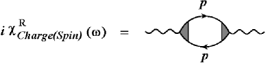
Figure 4: The Feynman diagram associated with the renormalized uniform charge and spin susceptibilities.

3 The 2D repulsive Hubbard model

3.1 The two-loop RG approach

Our two-loop RG calculation worked quite well in reproducing some low-energy properties of the 1D HM such as the gapless nature of the resulting in both charge and spin excitation spectra. This result encourages us to try to apply the same approach for problems, in which there are no known exact solutions to this present date. This is what happens very generally in strongly correlated 2D models, due to the fact that well-known analytical techniques such as the bosonization and the Bethe ansatz are not easily extendable to such higher-dimensional systems. Here, we discuss the application of the two-loop RG method developed earlier to the 2D repulsive HM slightly away from half-filling.

In 2D, the repulsive ($U>0$) Hubbard Hamiltonian defined on a square lattice is given in momentum space by

$$H=\sum_{\mathbf{k},\sigma}\xi_{\mathbf{k}}\psi^{\dagger}_{\mathbf{k}\sigma}\psi_{\mathbf{k}\sigma}+\left(\frac{U}{N_{sites}}\right)\sum_{\mathbf{p},\mathbf{k},\mathbf{q}}\psi^{\dagger}_{\mathbf{p}+\mathbf{k}-\mathbf{q}\uparrow}\psi^{\dagger}_{\mathbf{q}\downarrow}\psi_{\mathbf{k}\downarrow}\psi_{\mathbf{p}\uparrow},$$ (20)

where the energy dispersion is given by $\xi_{\mathbf{k}}=-2t\left[\cos(k_{x}a)+\cos(k_{y}a)\right]-\mu$, and $\psi^{\dagger}_{\mathbf{k}\sigma}$ and $\psi_{\mathbf{k}\sigma}$ are the creation and annihilation operators of electrons with momentum $\mathbf{k}=(k_{x},k_{y})$ and spin projection ${\sigma}=\uparrow,\downarrow$. The other definitions follow those of the 1D model, i.e., $\mu$ stands for the chemical potential, $N_{sites}$ is the number of total sites, and $a$ is the spacing of the 2D lattice. A very important difference here is the width of the noninteracting band, which is now given by $W=8t$.

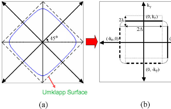
Figure 5: (a) The half-filled Fermi surface (FS) of the 2D Hubbard model (dashed line), the lightly hole-doped FS (solid line), and (b) the latter FS after a rotation of the axes by $45^{o}$ degrees.

The electron band filling of the system is controlled by the ratio $\mu/t$. When $\mu/t=0$ the model is exactly at half-filling condition. As we start doping it with holes, $\mu/t$ takes slightly negative values. As we can see from Fig. 5 (a), the FS of such lightly doped system is nearly flat, and contains no van Hove singularities in it. That FS will be our starting point for the two-loop RG approach. However, this 2D problem has additional complications compared to the 1D case, since we need now two momenta $k_{x}$ and $k_{y}$ to prescribe a renormalization procedure towards the FS. To simplify the calculations, we can perform a simple rotation of the axes by $45^{o}$ degrees, and change these two components by a component parallel ($k_{\parallel}$) and another perpendicular ($k_{\perp}$) to the FS. As a result of this, the 2D problem will bear a more transparent resemblance to the 1D case (see Fig. 5 (b)), and we can use the machinery developed in the previous section with some minor adaptations. To emphasize further the similarities of both problems, we divide the 2D FS into four different regions (two sets of solid and dashed line patches). Here, we restrict the momenta at the FS to the flat parts only. Analogously to the 1D problem, the interaction processes connecting parallel patches of the FS are always logarithmically IR divergent due to quantum fluctuations. In contrast, those connecting perpendicular patches always remain finite, and do not contribute to the RG flow equations in our approach. For convenience, we restrict ourselves to one-electron states labeled by the momenta $k_{\parallel}=k_{x}$ and $k_{\perp}=k_{y}$ associated with one of the two sets of perpendicular patches. The momenta parallel to the FS are restricted to the interval $-\Delta\leq k_{\parallel}\leq\Delta$, with $2\Delta$ being essentially the size of the flat patches. The energy dispersion of the single-particle states is given by $\xi_{\mathbf{k}}=v_{F}\left(\left|k_{\perp}\right|-k_{F}\right)$, and depends only on the momenta perpendicular to the FS. We define a label $a=\pm$ which refers to the flat sectors at $k_{\perp}=\pm k_{F}$, respectively. In addition, we take $k_{F}-\lambda\leq\left|k_{\perp}\right|\leq k_{F}+\lambda$, where $\lambda$ is the fixed ultraviolet (UV) microscopic momentum cut-off with $\Omega=2v_{F}\lambda$.

In the same spirit as before, we now write down the Lagrangian of the 2D HM as

$$L=\sum_{\textbf{k},\sigma,a=\pm}\psi_{(a)\sigma}^{\dagger}\left(\textbf{k},t\right)\left[i\partial_{t}-v_{F}\left(\left|k_{\perp}\right|-k_{F}\right)\right]\psi_{(a)\sigma}\left(\textbf{k},t\right)$$

$$-\frac{1}{V}\sum_{\textbf{p},\textbf{q},\textbf{k}}\sum_{\alpha,\beta,\gamma,\delta}\left[g_{2}\delta_{\alpha\delta}\delta_{\beta\gamma}-g_{1}\delta_{\alpha\gamma}\delta_{\beta\delta}\right]\psi_{\left(+\right)\delta}^{\dagger}\left(\textbf{p}+\textbf{q}-\textbf{k},t\right)\psi_{\left(-\right)\gamma}^{\dagger}\left(\textbf{k},t\right)\psi_{\left(-\right)\beta}\left(\textbf{q},t\right)\psi_{\left(+\right)\alpha}\left(\textbf{p},t\right),$$

(21)

where all the definitions follow the 1D HM case with $\psi^{\dagger}_{(\pm)}$ and $\psi_{(\pm)}$ being fermionic fields associated to electrons located at the $\pm$ patches and the summation over momenta being appropriately understood as $\sum_{\mathbf{p}}=V/(2\pi)^{2}\int d^{2}\mathbf{p}$ in the thermodynamic limit. Since this should represent the 2D HM, the Lagrangian is also written in a manifestly $SU(2)$ invariant form and the couplings are initially defined as $g_{1}=g_{2}=(V/4N_{sites})U$. In addition, we again neglect Umklapp processes here. This choice is related to the fact that we are mainly interested in dealing with the HM slightly away from half-filling and, therefore, our FS does not intersect the so-called Umklapp surface at any point (see again Fig. 5 (a)).

Apart from its physical importance especially regarding the possible explanation of high-Tc superconductivity, this 2D model is also very interesting from an exclusive RG point of view. In fact, when one deals with this FS model, the counterterms needed to renormalize the theory turn out to be continuous functions of the momenta parallel to the FS, rather than being simply infinite shifts. As a result, the couplings initially defined as constants in the 2D Hubbard Lagrangian acquire a momentum dependence and become renormalized functions of the three parallel momenta when one takes the system towards the FS. Thus, the new prescriptions become

$$\psi_{(a)\sigma} \rightarrow\psi_{(a)\sigma}^{R}+\Delta\psi_{(a)\sigma}^{R}(k_{\parallel})=Z^{1/2}(k_{\parallel})\psi_{(a)\sigma}^{R},$$ (22)

$$g_{i} \rightarrow\prod_{i=1}^{4}Z^{-1/2}(p_{i\parallel})\left[g_{iR}(p_{1\parallel},p_{2\parallel},p_{3\parallel})+\Delta g_{iR}(p_{1\parallel},p_{2\parallel},p_{3\parallel})\right].$$ (23)

where $p_{4\parallel}=p_{1\parallel}+p_{2\parallel}-p_{3\parallel}$. As before, there are still several ways to define the appropriate counterterms using the above prescription. In order to solve this, we establish renormalization conditions for the one-particle irreducible four-point functions as follows [11]

$$\Gamma^{(4)}(p_{1\parallel},p_{2\parallel},p_{3\parallel},p_{01}+p_{02}=p_{03}-p_{01}=\omega,p_{1}=p_{3}=-p_{2}=-p_{4}=k_{F})=-ig_{1R}(p_{1\parallel},p_{2\parallel},p_{3\parallel};\omega),$$ (24)

$$\Gamma^{(4)}(p_{1\parallel},p_{2\parallel},p_{3\parallel},p_{01}+p_{02}=p_{03}-p_{01}=\omega,p_{1}=p_{4}=-p_{2}=-p_{3}=k_{F})=-ig_{2R}(p_{1\parallel},p_{2\parallel},p_{3\parallel};\omega),$$ (25)

and also for the one-particle irreducible two-point function as

$$\Gamma^{(2)}(k_{0}=\omega,k=k_{F},k_{\parallel})=\omega,$$ (26)

where $\omega$ is again the energy scale which denotes the proximity of the renormalized theory to the FS.

Following the same procedure explained before, the corresponding RG flow equations for the couplings and quasiparticle weight of this 2D problem become coupled integro-differential equations, which are impossible to solve analytically. Therefore, one must solve them using a numerical approach. We choose here the standard fourth-order Runge-Kutta method. We refer the reader to our paper [11] for more details.

When one considers moderate initial interactions, the corresponding quasiparticle weight $Z$ becomes suppressed as one approaches the FS. This is a strong indicative that the resulting low-energy effective theory does not contain low-lying electronic quasiparticles in the system. In addition to this, instead of the renormalized coupling functions diverging as happens in well-known one-loop RG flows, they flow, for some particular choices of momenta, to strong coupling plateau values. This result means that those systems belong to the same universality class of a strongly coupled theory, whose detailed information must be determined from a consistent RG calculation of other quantities such as the uniform susceptibilities as we have done explicitly for the 1D HM case. In fact, we will see here that the suppression of the quasiparticle weight of the system will produce interesting effects in the RG flows of those quantities [14].

First, we must calculate the linear response due to an infinitesimal external field perturbation as before. Again, we add to the Lagrangian the following term

$$-h_{external}\sum_{\mathbf{p},a=\pm}\mathcal{T}_{\alpha}(\mathbf{p})\psi_{(a)\alpha}^{B\dagger}\left(\mathbf{p}\right)\psi^{B}_{(a)\alpha}\left(\mathbf{p}\right),$$ (27)

This will generate an additional vertex (the one-particle irreducible uniform response function $\Gamma^{(2,1)}(\mathbf{p},\mathbf{q}\approx 0)$), which will in turn be afflicted by divergences given by the Feynman diagrams of Fig. 3 as in the 1D case. Therefore, we rewrite the bare quantity $\mathcal{T}_{\alpha}$ in terms of its renormalized parameter $\mathcal{T}_{\alpha}$ and an appropriate counterterm $\Delta\mathcal{T}_{\alpha}$ as follows

$$\mathcal{T}_{\alpha}(p_{\parallel})=Z^{-1}(p_{\parallel})\left[\mathcal{T}^{R}_{\alpha}(p_{\parallel})+\Delta\mathcal{T}^{R}_{\alpha}(p_{\parallel})\right].$$ (28)

where the Z function is given by [11]

$$Z(p_{\parallel})=1-\frac{1}{32\pi^{4}v_{F}^{2}}\int dk_{\parallel}dq_{\parallel}[2g_{2R}\circ g_{2R}+2g_{1R}\circ g_{1R}-g_{1R}\circ g_{2R}-g_{2R}\circ g_{1R}]\ln\left(\frac{\Omega}{\omega}\right).$$ (29)

where the sign $\circ$ means that we are omitting the momentum dependence of the renormalized coupling functions. As was already mentioned, $\Delta\mathcal{T}_{\alpha}$ must absorb the divergences generated by the Feynman diagrams of Fig. 3. However, we may still define that counterterm in several ways. To solve this ambiguity, we make a prescription establishing precisely that the $\mathcal{T}^{R}_{\alpha}$ is the experimentally observable response, i.e., $\Gamma^{(2,1)}(p_{\parallel},p_{0}=\omega,p_{\perp}=k_{F};\textbf{q}\approx 0)=-i\mathcal{T}^{R}_{\alpha}(p_{\parallel},\omega)$, where $\omega$ is the RG energy scale parameter.

Now we turn to the definition of the two different types of uniform response functions, which arise from the symmetrization with respect to the spin projection $\alpha$, i.e.

$$\mathcal{T}^{R}_{Charge}(p_{\parallel},\omega) = \mathcal{T}^{R}_{\uparrow}(p_{\parallel},\omega)+\mathcal{T}^{R}_{\downarrow}(p_{\parallel},\omega),$$ (30)

$$\mathcal{T}^{R}_{Spin}(p_{\parallel},\omega) = \mathcal{T}^{R}_{\uparrow}(p_{\parallel},\omega)-\mathcal{T}^{R}_{\downarrow}(p_{\parallel},\omega),$$ (31)

where $\mathcal{T}^{R}_{Charge}$ and $\mathcal{T}^{R}_{Spin}$ are the uniform response functions associated with the charge and spin channels, respectively. To compute the RG flow equations of these response functions, one needs to recall that the bare parameters are independent of the renormalization scale $\omega$. Thus, using the RG condition $\omega d\mathcal{T}_{\alpha}/d\omega=0$, we obtain [14]

$$\omega\frac{d}{d\omega}\mathcal{T}^{R}_{Charge}(p_{\parallel})=\frac{1}{32\pi^{4}v_{F}^{2}}\bigg{(}\int dk_{\parallel}dq_{\parallel}[2g_{2R}\circ g_{2R}+2g_{1R}\circ g_{1R}+g_{1R}\circ g_{2R}+g_{2R}\circ g_{1R}$$

$$+g_{1R}\circ g_{2R}+g_{2R}\circ g_{1R}-2g_{2R}\circ g_{2R}-2g_{1R}\circ g_{1R}-2g_{2R}\circ g_{2R}-2g_{1R}\circ g_{1R}]\mathcal{T}^{R}_{Charge}(q_{\parallel})$$

$$+\int dk_{\parallel}dq_{\parallel}[2g_{2R}\circ g_{2R}+2g_{1R}\circ g_{1R}-g_{1R}\circ g_{2R}-g_{2R}\circ g_{1R}]\mathcal{T}^{R}_{Charge}(p_{\parallel})\bigg{)},$$ (32)

$$\omega\frac{d}{d\omega}\mathcal{T}^{R}_{Spin}(p_{\parallel})=\frac{1}{32\pi^{4}v_{F}^{2}}\bigg{(}\int dk_{\parallel}dq_{\parallel}[g_{1R}\circ g_{2R}+g_{2R}\circ g_{1R}+g_{1R}\circ g_{2R}+g_{2R}\circ g_{1R}$$

$$-2g_{2R}\circ g_{2R}-2g_{1R}\circ g_{1R}-2g_{2R}\circ g_{2R}-2g_{1R}\circ g_{1R}]\mathcal{T}^{R}_{Spin}(q_{\parallel})+\mathcal{T}^{R}_{Spin}(p_{\parallel})$$

$$\times\int dk_{\parallel}dq_{\parallel}[2g_{2R}\circ g_{2R}+2g_{1R}\circ g_{1R}-g_{1R}\circ g_{2R}-g_{2R}\circ g_{1R}]\bigg{)},$$ (33)

where the sign $\circ$ represents again the momentum dependence of the renormalized coupling functions which were omitted for convenience. To find the solutions for these RG equations, we resort to the same numerical method as described before.

Finally, once the response functions are obtained, we can calculate the flow of the uniform charge and spin susceptibilities of the system. They are given by the same diagram as in the 1D case (Fig. 4). Therefore, we have

$$\chi^{R}_{Charge(Spin)}(\omega)=\frac{1}{4\pi^{2}v_{F}}\int_{-\Delta}^{\Delta}dp_{\parallel}\left[\mathcal{T}^{R}_{Charge(Spin)}(p_{\parallel},\omega)\right]^{2}.\\$$ (34)

Once more, we use the same numerical procedure to estimate those quantities. Our results are displayed in Fig. 6. We note in this plot that both uniform susceptibilities flow at the same rate as we approach the FS. As a result, again, there is no spin-charge separation effects in this model. One way to possibly circumvent this would be to add $g_{4}$-type interaction contributions and work hard to implement an appropriate RG scheme in this system (for this question, see also Ref. [15] for a discussion of a closely related problem in 1D). Notice that, for moderate initial couplings with $Z$ going to zero, the susceptibilities become strongly suppressed in the same low-energy limit in markedly contrast to the 1D case, where they remain finite. Therefore, our result adds further support to the interpretation that the low-energy effective theory for those cases should be a fully gapped state in both charge and spin excitation spectra [14]. Since such an effective theory has only gapful excitations present, it cannot be related to any spontaneously broken symmetry state. Consequently, it should stay in a liquid phase-like state associated with a short-range order in the system. These effects become even more transparent when we calculate the susceptibilities associated with several order parameters (see Ref. [16]). There, we show that all susceptibilities are finite as we vary the RG energy scale. Thus, it is not possible to any given order to become long-range correlated in this 2D system. This unusual quantum state predicted long ago by Anderson is commonly referred to as an insulating spin liquid (ISL), and it is widely believed to play a central role in the appropriate explanation of the underlying mechanism of high-Tc superconductivity.

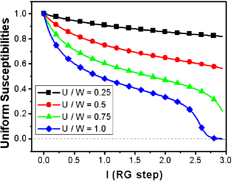
Figure 6: The RG flow of the uniform charge and spin susceptibilities as we increase the bare interaction strength given by $U=(g/\pi v_{F})t$. Our RG step $l$ is given by $l=\ln(\Omega/\omega)$.

3.2 The RPA approach

We now compare the two-loop RG result with another approach for calculating the uniform susceptibilities that appears widely in the literature [17, 18], i.e., the random phase approximation (RPA). This method is used for estimating those quantities at an one-loop RG level. At this order, the renormalized couplings are known to diverge at finite energy scales, below which the RG is simply unable to access. The approximation consists of the assumption that the remaining information is given by the one-loop diagrams of the uniform response functions (see Fig. 7). However, since these diagrams are not IR divergent, it is not possible to derive RG flow equations for those quantities at this order. The resulting equations will be integral equations which must be solved self-consistently in strong contrast to our previous two-loop RG approach, which allowed us to derive proper flow equations.

Let us consider Eq. (26). If one goes only up to one-loop order, the quasiparticle weight $Z$ must be equal to unity, since one is not taking into account self-energy corrections in the calculations. In this way, we have

$$\mathcal{T}_{\alpha}(p_{\parallel})=\mathcal{T}^{R}_{\alpha}(p_{\parallel})+\Delta\mathcal{T}^{R}_{\alpha}(p_{\parallel}).$$ (35)

Now, calculating the Feynman diagrams of Fig. 7 and establishing the same renormalization condition used in the previous section, i.e., $\Gamma^{(2,1)}(p_{\parallel},p_{0}=\omega,p_{\perp}=k_{F};\textbf{q}\approx 0)=-i\mathcal{T}^{R}_{\alpha}(p_{\parallel},\omega)$, we obtain the following expression

$$\mathcal{T}^{R}_{\alpha}(p_{\parallel})=\mathcal{T}_{\alpha}(p_{\parallel})+\frac{1}{2\pi v_{F}}\int_{-\Delta}^{\Delta}dk_{\parallel}\left[\mathcal{T}^{R}_{\alpha}(k_{\parallel})g_{1R}(p_{\parallel},k_{\parallel},p_{\parallel})-\sum_{\sigma}\mathcal{T}^{R}_{\sigma}(k_{\parallel})g_{2R}(p_{\parallel},k_{\parallel},k_{\parallel})\right].$$ (36)

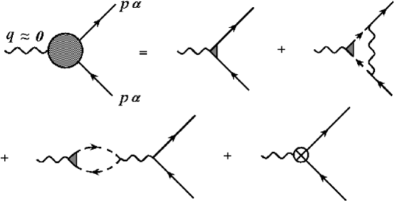
Figure 7: The Feynman diagrams for the calculation of the uniform response functions within the RPA approach.

We note here that this equation is indeed not a RG flow equation. Thus, symmetrizing this quantity with respect to the spin projection $\alpha$, i.e.

$$\mathcal{T}^{R}_{Charge}(p_{\parallel},\omega) = \mathcal{T}^{R}_{\uparrow}(p_{\parallel},\omega)+\mathcal{T}^{R}_{\downarrow}(p_{\parallel},\omega),$$ (37)

$$\mathcal{T}^{R}_{Spin}(p_{\parallel},\omega) = \mathcal{T}^{R}_{\uparrow}(p_{\parallel},\omega)-\mathcal{T}^{R}_{\downarrow}(p_{\parallel},\omega),$$ (38)

we obtain for the uniform charge and spin response functions the following equations

$$\mathcal{T}^{R}_{Charge}(p_{\parallel};\omega) = \mathcal{T}_{Charge}(p_{\parallel})+\frac{1}{2\pi v_{F}}\int_{-\Delta}^{\Delta}dk_{\parallel}\mathcal{T}^{R}_{Charge}(k_{\parallel})$$

$$\times\left[g_{1R}(p_{\parallel},k_{\parallel},p_{\parallel};\omega)-2g_{2R}(p_{\parallel},k_{\parallel},k_{\parallel};\omega)\right],$$

$$\mathcal{T}^{R}_{Spin}(p_{\parallel};\omega) = \mathcal{T}_{Spin}(p_{\parallel})+\frac{1}{2\pi v_{F}}\int_{-\Delta}^{\Delta}dk_{\parallel}\mathcal{T}^{R}_{Spin}(k_{\parallel})g_{1R}(p_{\parallel},k_{\parallel},p_{\parallel};\omega).$$

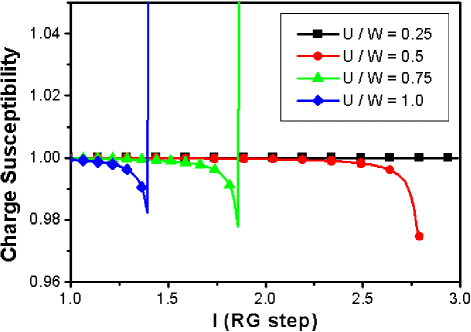
Figure 8: The RG flow of the uniform charge susceptibility as we increase the bare interaction strength given by $U=(g/\pi v_{F})t$ within the RPA approach. Our RG step $l$ is given by $l=\ln(\Omega/\omega)$.

which now must be calculated self-consistently. Here, we discretize the FS in exactly the same way as explained in the previous section.

Once these quantities are estimated, we can calculate the uniform susceptibilities in the RPA approximation, i.e.

$$\chi^{(RPA)}_{Charge(Spin)}(\omega)=\frac{1}{4\pi^{2}v_{F}}\int_{-\Delta}^{\Delta}dp_{\parallel}\left[\mathcal{T}^{R}_{Charge(Spin)}(p_{\parallel},\omega)\right]^{2}.\\$$ (41)

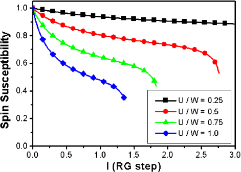
Figure 9: The RG flow of the uniform spin susceptibility as we increase the bare interaction strength given by $U=(g/\pi v_{F})t$ within the RPA approach. Our RG step $l$ is given by $l=\ln(\Omega/\omega)$.

The results for these quantities are displayed in Figs. 8 and 9. In the charge susceptibility plot, although the initial flow gives the impression that it becomes somewhat suppressed as we approach the FS, we observe in fact a strong upturn of the flow towards infinity in qualitative agreement with other numerical results [17, 18]. As for the uniform spin susceptibility, we note a tendency to flow to zero in the low-energy limit as we increase the initial coupling $U$. Therefore, even though one might argue that the RPA approach captures an initial tendency of both quantities to become suppressed, this is in fact rather approximate. As a result, one is not able to detect clearly the formation of the ISL state in this 2D model within this approximation.

In contrast, our two-loop RG calculation provided a more solid evidence that the natural candidate for the low-energy effective description of the 2D HM slightly away from half-filling is indeed the ISL. The underlying reason for the different behavior of the two approaches lies in the following physical principle. Quantum fluctuation effects are well-known to be very effective in destroying long-range correlations especially in low-dimensional systems. In fact, the more fluctuations are taken into account, the more likely long-range ordered states are transformed into short-range ordered ones. This also becomes clear as a result of our work. In accordance with this, we can infer that if we were to consider higher-order fluctuations such as a three-loop RG calculation or beyond, we would approach the ISL state even more rapidly in this 2D HM system.

4 Conclusions

Here we investigated the renormalization of the uniform charge and spin susceptibilities of the 2D HM slightly away from half-filling within a two-loop RG approach. In our calculations, we took into account simultaneously both the renormalization of the couplings and self-energy effects. As a warm-up example, we first applied this approach to the 1D HM away from half-filling and reproduced several features associated with the Luttinger liquid fixed-point: the irrelevance in the RG sense of the so-called backscattering interaction processes, the complete absence of low-lying quasiparticles in the vicinity of the FS, and finally the finiteness of the both charge and spin uniform susceptibilities indicating that the resulting state is indeed metallic.

Once the RG technique was explained in detail, we moved on to the problem we were mostly interested in, i.e., the 2D HM for densities slightly away from half-filling condition. We emphasized the strong similarities to the 1D case, and adapted the technique to deal properly with this 2D model. We pointed out that, for moderate bare interaction $U$, the coupling functions flow to strong-coupling plateau values for particular choices of the external momenta. Besides, this regime is also characterized by a strongly suppressed quasiparticle weight $Z$, which is a strong indicative of the absence of low-lying electronic quasiparticles in the resulting low-energy effective theory. Then, in order to extract further information about this state, we calculated the uniform susceptibilities associated with the charge and spin degrees of freedom, and showed that both quantities renormalize to zero in the low-energy limit. This result implies that both charge and spin excitation spectra are fully gapped, and the resulting state should be given by an insulating spin liquid.

In order to compare our result with other numerical estimates encountered in the literature, we derived a RPA approach to calculate the uniform susceptibilities within a one-loop RG scheme. As a result, we reproduced the well-known one-loop results, and showed that they were in fact not sufficient to obtain in a clear way the ISL low-energy effective theory in this case. This should be contrasted with the two-loop RG approach, where we do observe this state. We explained that the physical reason for the discrepancies of both results is that, in this particular 2D problem, one must add more quantum fluctuations in order to effectively remove every single instability that could potentially develop into long-range order in the system. Therefore, if one could go beyond two-loop RG order, one would not change this picture qualitatively, and might well approach the ISL state even more rapidly.

This work was partially supported by the Fundação de Empreendimentos Científicos e Tecnológicos (FINATEC) and by the Conselho Nacional de Desenvolvimento Científico e Tecnológico (CNPq).

References

- [1] Landau L D 1957 Sov. Phys. - JETP 3 920; 5 101; 1959 Sov. Phys. - JETP 8 70
- [2] Nozieres P 1964 Interacting Fermi Systems (New York: Benjamin)
- [3] Nambu Y 1960 Phys. Rev. Lett. 4 380
- [4] Goldstone J 1961 Nuovo Cimento 19 154
- [5] Anderson P W 1973 Mater. Res. Bull. 8 153; Fazekas P and Anderson P W 1974 Philos. Mag. 30 432
- [6] Anderson P W 1987 Science 235 1196
- [7] Solyom J 1979 Adv. Phys. 28 201
- [8] Haldane F D M 1981 J. Phys. C: Solid State Phys. 14 2585
- [9] Voit J 1995 Rep. Prog. Phys. 58 977
- [10] The name insulating spin liquid refers to a liquid phase-like state, which is fully gapped in both charge and spin excitation spectra. Therefore, it cannot be related to any broken symmetry state and, as a consequence, should possess only short-range order.
- [11] Freire H, Correa E and Ferraz A 2005 Phys. Rev. B 71 165113
- [12] Peskin M E and Schroeder D V 1995, “An Introduction to Quantum Field Theory” (Reading, Massachusetts: Perseus Books)
- [13] Benfatto G and Mostropietro V 2005, Commun. Math. Phys. 258 609
- [14] Freire H, Correa E and Ferraz A 2006, Phys. Rev. B 73, 073103
- [15] See, e.g., Ferraz A, arXiv:cond-mat/0512098 (to appear in J. Phys. A: Math. and Gen.)
- [16] Correa E, Freire H and Ferraz A, arXiv:cond-mat/0512626
- [17] Halboth C J and Metzner W 2000 Phys. Rev. B 61 7364
- [18] Honerkamp C, Salmhofer M, Furukawa N and Rice T M 2001 Phys. Rev. B 63 35109