The dynamic impedance of a sphere oscillating in an elastic medium is considered. Oestreicher’s [1] formula for the impedance of a sphere bonded to the surrounding medium can be expressed simply in terms of three lumped impedances associated with the displaced mass and the longitudinal and transverse waves. If the surface of the sphere slips while the normal velocity remains continuous, the impedance formula is modified by adjusting the definition of the transverse impedance to include the interfacial impedance.

Short title: Thermoelastic thin plates

Contact:
norris@rutgers.edu
ph. 1.732.445.3818
fax 1.732.445.3124

1 Introduction

The dynamic impedance of a spherical particle embedded in a medium is important for acoustical measurement and imaging. The impedance is used, for instance, in measurement of the mechanical properties of tissue, e.g. [2], and is intimately related to the radiation forcing on particles [3]. The latter is the basis for imaging techniques such as vibro-acoustography which has considerable potential in mammography for detection of microcalcifications in breast tissue [4]. Oestreicher [1] derived the impedance for a rigid sphere oscillating in a viscoelastic medium over 50 years ago. Although it was derived for a sphere in an infinite medium, Oestreicher’s formula is also applicable, with minor modification [5], to dynamical indentation techniques where the particle is in contact with the surface of the specimen, see Zhang et al. [6] for a review of related work. Chen et al. [7] recently validated Oestreicher’s formula experimentally by measuring the dynamic radiation force on a sphere in a fluid. The impedance formula is based on perfect no slip conditions between the spherical inclusion and its surroundings. This may not always be a valid assumption, e.g., in circumstances where a foreign object is embedded in soft material. This was precisely the situation in recent measurements of the viscosity of DNA cross-linked gels by magnetic forcing on a small steel sphere [8]. This paper generalizes the impedance formula to include the possibility of dynamic slip.

Two related results are derived in this paper. The first is a modified form of Oestreicher’s formula which enables it to be interpreted in terms of lumped parameter impedances. This leads to a simple means to consider the more general case of a sphere oscillating in a viscoelastic medium which is permitted to slip relative to its surroundings. The slip is characterized by an interfacial impedance which relates the shear stress to the discontinuity in tangential velocities. This generalization includes Oestreicher’s original formula as the limit of infinite interfacial impedance, and agrees with previous results for the static stiffness of a spherical inclusion with and without slip [9].

2 Summary of results

A sphere undergoes time harmonic oscillatory motion of amplitude $u_{0}$ in the direction $\hat{\mathchoice{\mbox{\boldmath$\displaystyle\mathbf{x}$}}{\mbox{\boldmath$\textstyle\mathbf{x}$}}{\mbox{\boldmath$\scriptstyle\mathbf{x}$}}{\mbox{\boldmath$\scriptscriptstyle\mathbf{x}$}}}$,

$${\mathchoice{\mbox{\boldmath$\displaystyle\mathbf{u}$}}{\mbox{\boldmath$\textstyle\mathbf{u}$}}{\mbox{\boldmath$\scriptstyle\mathbf{u}$}}{\mbox{\boldmath$\scriptscriptstyle\mathbf{u}$}}}^{\text{s}phere}=u_{0}\,e^{-i\omega t}\,\hat{\mathchoice{\mbox{\boldmath$\displaystyle\mathbf{x}$}}{\mbox{\boldmath$\textstyle\mathbf{x}$}}{\mbox{\boldmath$\scriptstyle\mathbf{x}$}}{\mbox{\boldmath$\scriptscriptstyle\mathbf{x}$}}}.$$ (1)

The time harmonic factor $e^{-i\omega t}$ is omitted but understood in future expressions. The sphere, which is assumed to be rigid and of radius $a$, is embedded in an elastic medium of infinite extent with mass density $\rho$ and Lamé moduli $\lambda$ and $\mu$. The moduli may be real or complex, corresponding to an elastic or viscoelastic solid. We will later consider complex shear modulus $\mu=\mu_{1}-i\omega\mu_{2}$, where the imaginary term dominates in a viscous medium. The force exerted on the sphere by the surrounding medium acts in the $\hat{\mathchoice{\mbox{\boldmath$\displaystyle\mathbf{x}$}}{\mbox{\boldmath$\textstyle\mathbf{x}$}}{\mbox{\boldmath$\scriptstyle\mathbf{x}$}}{\mbox{\boldmath$\scriptscriptstyle\mathbf{x}$}}}$-direction, and is defined by

$$F\hat{\mathchoice{\mbox{\boldmath$\displaystyle\mathbf{x}$}}{\mbox{\boldmath$\textstyle\mathbf{x}$}}{\mbox{\boldmath$\scriptstyle\mathbf{x}$}}{\mbox{\boldmath$\scriptscriptstyle\mathbf{x}$}}}=\int\limits_{r=a}{\mathchoice{\mbox{\boldmath$\displaystyle\mathbf{T}$}}{\mbox{\boldmath$\textstyle\mathbf{T}$}}{\mbox{\boldmath$\scriptstyle\mathbf{T}$}}{\mbox{\boldmath$\scriptscriptstyle\mathbf{T}$}}}\,{\text{d}}s\,,$$ (2)

where $\textstyle\mathbf{T}$ is the traction vector on the surface. The sphere impedance is defined

$$Z=\frac{F}{-i\omega u_{0}}.$$ (3)

Oestreicher’s expression for the impedance of a sphere that does not slip relative to the elastic medium is [1]

$$Z=\frac{4}{3}\pi a^{3}\rho\,i\omega\,\bigg{[}\bigr{(}1+\frac{3i}{ah}-\frac{3}{a^{2}h^{2}}\bigr{)}-2\bigr{(}\frac{-i}{ah}+\frac{1}{a^{2}h^{2}}\bigr{)}\bigr{(}3-\frac{a^{2}k^{2}}{1-iak}\bigr{)}\bigg{]}\bigg{/}$$

$$\qquad\qquad\qquad\qquad\bigg{[}\bigr{(}\frac{-i}{ah}+\frac{1}{a^{2}h^{2}}\bigr{)}\frac{a^{2}k^{2}}{1-iak}+\bigr{(}2-\frac{a^{2}k^{2}}{1-iak}\bigr{)}\bigg{]}\,.$$ (4)

Here $k$ and $h$ are, respectively, the longitudinal and transverse wavenumbers, $k=\omega/c_{L}$, $h=\omega/c_{T}$ with $c_{L}=\sqrt{(\lambda+2\mu)/\rho}$ and $c_{T}=\sqrt{\mu/\rho}$.

Noting that Oestreicher’s formula can be rewritten

$$Z=\frac{4}{3}\pi a^{3}\rho\,i\omega\,\bigg{\{}-1+\bigg{[}\frac{1}{3}\bigr{(}1-\frac{3(1-ika)}{k^{2}a^{2}}\bigr{)}^{-1}+\frac{2}{3}\bigr{(}1-\frac{3(1-iha)}{h^{2}a^{2}}\bigr{)}^{-1}\bigg{]}^{-1}\bigg{\}}\,,$$ (5)

implies our first result, that the impedance satisfies

$$\frac{3}{Z+Z_{\text{m}}}=\frac{1}{Z_{L}+Z_{\text{m}}}+\frac{2}{Z_{T}+Z_{\text{m}}}\,,$$ (6)

where the three additional impedances are defined as

$$Z_{\text{m}} =i\omega\,\frac{4}{3}\pi a^{3}\rho,$$ (7a)

$$Z_{L} =(i\omega)^{-1}4\pi a(\lambda+2\mu)\,(1-ika),$$ (7b)

$$Z_{T} =(i\omega)^{-1}\,4\pi a\mu(1-iha).$$ (7c)

The second result is that if the sphere is allowed to slip relative to the elastic medium then the general form of eq. (6) is preserved with $Z_{T}$ modified. Specifically, suppose the tangential component of the traction satisfies

$${\mathchoice{\mbox{\boldmath$\displaystyle\mathbf{T}$}}{\mbox{\boldmath$\textstyle\mathbf{T}$}}{\mbox{\boldmath$\scriptstyle\mathbf{T}$}}{\mbox{\boldmath$\scriptscriptstyle\mathbf{T}$}}}\cdot\hat{\mathchoice{\mbox{\boldmath$\displaystyle\mathbf{t}$}}{\mbox{\boldmath$\textstyle\mathbf{t}$}}{\mbox{\boldmath$\scriptstyle\mathbf{t}$}}{\mbox{\boldmath$\scriptscriptstyle\mathbf{t}$}}}=z_{I}\,(\dot{\mathchoice{\mbox{\boldmath$\displaystyle\mathbf{u}$}}{\mbox{\boldmath$\textstyle\mathbf{u}$}}{\mbox{\boldmath$\scriptstyle\mathbf{u}$}}{\mbox{\boldmath$\scriptscriptstyle\mathbf{u}$}}}^{\text{s}phere}-{\mathchoice{\mbox{\boldmath$\displaystyle\mathbf{v}$}}{\mbox{\boldmath$\textstyle\mathbf{v}$}}{\mbox{\boldmath$\scriptstyle\mathbf{v}$}}{\mbox{\boldmath$\scriptscriptstyle\mathbf{v}$}}})\cdot\hat{\mathchoice{\mbox{\boldmath$\displaystyle\mathbf{t}$}}{\mbox{\boldmath$\textstyle\mathbf{t}$}}{\mbox{\boldmath$\scriptstyle\mathbf{t}$}}{\mbox{\boldmath$\scriptscriptstyle\mathbf{t}$}}},\qquad r=a,$$ (8)

where $\hat{\mathchoice{\mbox{\boldmath$\displaystyle\mathbf{t}$}}{\mbox{\boldmath$\textstyle\mathbf{t}$}}{\mbox{\boldmath$\scriptstyle\mathbf{t}$}}{\mbox{\boldmath$\scriptscriptstyle\mathbf{t}$}}}$ is a unit tangent vector, $\textstyle\mathbf{v}$ the velocity of the elastic medium adjacent to the sphere, and $z_{I}$ is an interfacial impedance, discussed later. Equation (8) holds at each point on the interface $r=a$. We find that $Z$ now satisfies

$$\frac{3}{Z+Z_{\text{m}}}=\frac{1}{Z_{L}+Z_{\text{m}}}+\frac{2}{Z_{S}+Z_{\text{m}}}\,,$$ (9)

where the new impedance $Z_{S}$ is given by

$$\frac{1}{Z_{S}}=\frac{1}{Z_{T}}+\frac{1}{4\pi a^{2}z_{I}+(i\omega)^{-1}\,8\pi a\mu}\,.$$ (10)

These results are derived in the next Section and discussed in Section 4.

3 Analysis

We use Oestreicher’s [1] representation for the elastic field outside the sphere,

$${\mathchoice{\mbox{\boldmath$\displaystyle\mathbf{u}$}}{\mbox{\boldmath$\textstyle\mathbf{u}$}}{\mbox{\boldmath$\scriptstyle\mathbf{u}$}}{\mbox{\boldmath$\scriptscriptstyle\mathbf{u}$}}}=-A_{1}\operatorname{grad}\big{(}\frac{h_{1}(kr)}{kr}x\big{)}+B_{1}\big{[}2h_{0}(hr)\operatorname{grad}x-h_{2}(hr)r^{3}\operatorname{grad}\frac{x}{r^{3}}\big{]},\qquad r\geq a,$$ (11)

where $r=|{\mathchoice{\mbox{\boldmath$\displaystyle\mathbf{r}$}}{\mbox{\boldmath$\textstyle\mathbf{r}$}}{\mbox{\boldmath$\scriptstyle\mathbf{r}$}}{\mbox{\boldmath$\scriptscriptstyle\mathbf{r}$}}}|$ is the spherical radius and $x$ is the component of $\textstyle\mathbf{r}$ in the $\hat{\mathchoice{\mbox{\boldmath$\displaystyle\mathbf{x}$}}{\mbox{\boldmath$\textstyle\mathbf{x}$}}{\mbox{\boldmath$\scriptstyle\mathbf{x}$}}{\mbox{\boldmath$\scriptscriptstyle\mathbf{x}$}}}-$direction, both with origin at the center of the sphere. Also, $h_{n}$ are spherical Hankel functions of the first kind [10]. Let $\hat{\mathchoice{\mbox{\boldmath$\displaystyle\mathbf{r}$}}{\mbox{\boldmath$\textstyle\mathbf{r}$}}{\mbox{\boldmath$\scriptstyle\mathbf{r}$}}{\mbox{\boldmath$\scriptscriptstyle\mathbf{r}$}}}=r^{-1}{\mathchoice{\mbox{\boldmath$\displaystyle\mathbf{r}$}}{\mbox{\boldmath$\textstyle\mathbf{r}$}}{\mbox{\boldmath$\scriptstyle\mathbf{r}$}}{\mbox{\boldmath$\scriptscriptstyle\mathbf{r}$}}}$ denote the unit radial vector, then

$${\mathchoice{\mbox{\boldmath$\displaystyle\mathbf{u}$}}{\mbox{\boldmath$\textstyle\mathbf{u}$}}{\mbox{\boldmath$\scriptstyle\mathbf{u}$}}{\mbox{\boldmath$\scriptscriptstyle\mathbf{u}$}}}=-A_{1}\big{[}\frac{h_{1}(kr)}{kr}\hat{\mathchoice{\mbox{\boldmath$\displaystyle\mathbf{x}$}}{\mbox{\boldmath$\textstyle\mathbf{x}$}}{\mbox{\boldmath$\scriptstyle\mathbf{x}$}}{\mbox{\boldmath$\scriptscriptstyle\mathbf{x}$}}}-h_{2}(kr)\frac{x}{r}\hat{\mathchoice{\mbox{\boldmath$\displaystyle\mathbf{r}$}}{\mbox{\boldmath$\textstyle\mathbf{r}$}}{\mbox{\boldmath$\scriptstyle\mathbf{r}$}}{\mbox{\boldmath$\scriptscriptstyle\mathbf{r}$}}}\big{]}+B_{1}\big{[}2h_{0}(hr)\hat{\mathchoice{\mbox{\boldmath$\displaystyle\mathbf{x}$}}{\mbox{\boldmath$\textstyle\mathbf{x}$}}{\mbox{\boldmath$\scriptstyle\mathbf{x}$}}{\mbox{\boldmath$\scriptscriptstyle\mathbf{x}$}}}-h_{2}(hr)(\hat{\mathchoice{\mbox{\boldmath$\displaystyle\mathbf{x}$}}{\mbox{\boldmath$\textstyle\mathbf{x}$}}{\mbox{\boldmath$\scriptstyle\mathbf{x}$}}{\mbox{\boldmath$\scriptscriptstyle\mathbf{x}$}}}-3\frac{x}{r}\hat{\mathchoice{\mbox{\boldmath$\displaystyle\mathbf{r}$}}{\mbox{\boldmath$\textstyle\mathbf{r}$}}{\mbox{\boldmath$\scriptstyle\mathbf{r}$}}{\mbox{\boldmath$\scriptscriptstyle\mathbf{r}$}}})\big{]}.$$ (12)

The surface traction is ${\mathchoice{\mbox{\boldmath$\displaystyle\mathbf{T}$}}{\mbox{\boldmath$\textstyle\mathbf{T}$}}{\mbox{\boldmath$\scriptstyle\mathbf{T}$}}{\mbox{\boldmath$\scriptscriptstyle\mathbf{T}$}}}={\mathchoice{\mbox{\boldmath$\displaystyle\mathbf{\sigma}$}}{\mbox{\boldmath$\textstyle\mathbf{\sigma}$}}{\mbox{\boldmath$\scriptstyle\mathbf{\sigma}$}}{\mbox{\boldmath$\scriptscriptstyle\mathbf{\sigma}$}}}\hat{\mathchoice{\mbox{\boldmath$\displaystyle\mathbf{r}$}}{\mbox{\boldmath$\textstyle\mathbf{r}$}}{\mbox{\boldmath$\scriptstyle\mathbf{r}$}}{\mbox{\boldmath$\scriptscriptstyle\mathbf{r}$}}}$ where $\textstyle\mathbf{\sigma}$ is the stress tensor. The traction can be calculated from (12) and the following identity [1] for an isotropic solid,

$${\mathchoice{\mbox{\boldmath$\displaystyle\mathbf{T}$}}{\mbox{\boldmath$\textstyle\mathbf{T}$}}{\mbox{\boldmath$\scriptstyle\mathbf{T}$}}{\mbox{\boldmath$\scriptscriptstyle\mathbf{T}$}}}=\hat{\mathchoice{\mbox{\boldmath$\displaystyle\mathbf{r}$}}{\mbox{\boldmath$\textstyle\mathbf{r}$}}{\mbox{\boldmath$\scriptstyle\mathbf{r}$}}{\mbox{\boldmath$\scriptscriptstyle\mathbf{r}$}}}\lambda\operatorname{div}{\mathchoice{\mbox{\boldmath$\displaystyle\mathbf{u}$}}{\mbox{\boldmath$\textstyle\mathbf{u}$}}{\mbox{\boldmath$\scriptstyle\mathbf{u}$}}{\mbox{\boldmath$\scriptscriptstyle\mathbf{u}$}}}+\frac{\mu}{r}\operatorname{grad}{\mathchoice{\mbox{\boldmath$\displaystyle\mathbf{r}$}}{\mbox{\boldmath$\textstyle\mathbf{r}$}}{\mbox{\boldmath$\scriptstyle\mathbf{r}$}}{\mbox{\boldmath$\scriptscriptstyle\mathbf{r}$}}}\cdot{\mathchoice{\mbox{\boldmath$\displaystyle\mathbf{u}$}}{\mbox{\boldmath$\textstyle\mathbf{u}$}}{\mbox{\boldmath$\scriptstyle\mathbf{u}$}}{\mbox{\boldmath$\scriptscriptstyle\mathbf{u}$}}}+\mu\big{(}\frac{\partial}{\partial r}-\frac{1}{r}\big{)}{\mathchoice{\mbox{\boldmath$\displaystyle\mathbf{u}$}}{\mbox{\boldmath$\textstyle\mathbf{u}$}}{\mbox{\boldmath$\scriptstyle\mathbf{u}$}}{\mbox{\boldmath$\scriptscriptstyle\mathbf{u}$}}}\,.$$ (13)

Thus, referring to (2), we have

$${\mathchoice{\mbox{\boldmath$\displaystyle\mathbf{T}$}}{\mbox{\boldmath$\textstyle\mathbf{T}$}}{\mbox{\boldmath$\scriptstyle\mathbf{T}$}}{\mbox{\boldmath$\scriptscriptstyle\mathbf{T}$}}}\cdot\hat{\mathchoice{\mbox{\boldmath$\displaystyle\mathbf{x}$}}{\mbox{\boldmath$\textstyle\mathbf{x}$}}{\mbox{\boldmath$\scriptstyle\mathbf{x}$}}{\mbox{\boldmath$\scriptscriptstyle\mathbf{x}$}}}= \big{[}2\mu h_{2}(kr)\big{(}1-3\frac{x^{2}}{r^{2}}\big{)}+(\lambda+2\mu)krh_{1}(kr)\frac{x^{2}}{r^{2}}\big{]}\,\frac{A_{1}}{r}$$

$$+\big{[}2h_{2}(hr)\big{(}1-3\frac{x^{2}}{r^{2}}\big{)}-hrh_{1}(hr)\big{(}1-\frac{x^{2}}{r^{2}}\big{)}\big{]}\,3\mu\frac{B_{1}}{r}\,.$$ (14)

Integrating over the sphere surface, the resultant is

$$F=\frac{4}{3}\pi a^{3}\rho\omega^{2}\,\big{[}A_{1}\frac{h_{1}(ka)}{ka}-6B_{1}\frac{h_{1}(ha)}{ha}\big{]}\,.$$ (15)

The coefficients $A_{1}$ and $B_{1}$ follow from the conditions describing the interaction of the sphere with its surroundings. These are the general slip condition (8) plus the requirement that the normal velocity is continuous. The conditions at the surface of the sphere are

$$\begin{split}{\mathchoice{\mbox{\boldmath$\displaystyle\mathbf{u}$}}{\mbox{\boldmath$\textstyle\mathbf{u}$}}{\mbox{\boldmath$\scriptstyle\mathbf{u}$}}{\mbox{\boldmath$\scriptscriptstyle\mathbf{u}$}}}\cdot\hat{\mathchoice{\mbox{\boldmath$\displaystyle\mathbf{r}$}}{\mbox{\boldmath$\textstyle\mathbf{r}$}}{\mbox{\boldmath$\scriptstyle\mathbf{r}$}}{\mbox{\boldmath$\scriptscriptstyle\mathbf{r}$}}}&=u_{0}\,\hat{\mathchoice{\mbox{\boldmath$\displaystyle\mathbf{x}$}}{\mbox{\boldmath$\textstyle\mathbf{x}$}}{\mbox{\boldmath$\scriptstyle\mathbf{x}$}}{\mbox{\boldmath$\scriptscriptstyle\mathbf{x}$}}}\cdot\hat{\mathchoice{\mbox{\boldmath$\displaystyle\mathbf{r}$}}{\mbox{\boldmath$\textstyle\mathbf{r}$}}{\mbox{\boldmath$\scriptstyle\mathbf{r}$}}{\mbox{\boldmath$\scriptscriptstyle\mathbf{r}$}}}\\ {\mathchoice{\mbox{\boldmath$\displaystyle\mathbf{T}$}}{\mbox{\boldmath$\textstyle\mathbf{T}$}}{\mbox{\boldmath$\scriptstyle\mathbf{T}$}}{\mbox{\boldmath$\scriptscriptstyle\mathbf{T}$}}}\cdot\hat{\mathchoice{\mbox{\boldmath$\displaystyle\mathbf{t}$}}{\mbox{\boldmath$\textstyle\mathbf{t}$}}{\mbox{\boldmath$\scriptstyle\mathbf{t}$}}{\mbox{\boldmath$\scriptscriptstyle\mathbf{t}$}}}&=i\omega z_{I}\,({\mathchoice{\mbox{\boldmath$\displaystyle\mathbf{u}$}}{\mbox{\boldmath$\textstyle\mathbf{u}$}}{\mbox{\boldmath$\scriptstyle\mathbf{u}$}}{\mbox{\boldmath$\scriptscriptstyle\mathbf{u}$}}}-u_{0}\hat{\mathchoice{\mbox{\boldmath$\displaystyle\mathbf{x}$}}{\mbox{\boldmath$\textstyle\mathbf{x}$}}{\mbox{\boldmath$\scriptstyle\mathbf{x}$}}{\mbox{\boldmath$\scriptscriptstyle\mathbf{x}$}}})\cdot\hat{\mathchoice{\mbox{\boldmath$\displaystyle\mathbf{t}$}}{\mbox{\boldmath$\textstyle\mathbf{t}$}}{\mbox{\boldmath$\scriptstyle\mathbf{t}$}}{\mbox{\boldmath$\scriptscriptstyle\mathbf{t}$}}}\end{split}\,\,\Biggr{\}}\qquad r=a.$$ (16)

By symmetry, the only non-zero tangential component is in the plane of $\hat{\mathchoice{\mbox{\boldmath$\displaystyle\mathbf{r}$}}{\mbox{\boldmath$\textstyle\mathbf{r}$}}{\mbox{\boldmath$\scriptstyle\mathbf{r}$}}{\mbox{\boldmath$\scriptscriptstyle\mathbf{r}$}}}$ and $\hat{\mathchoice{\mbox{\boldmath$\displaystyle\mathbf{x}$}}{\mbox{\boldmath$\textstyle\mathbf{x}$}}{\mbox{\boldmath$\scriptstyle\mathbf{x}$}}{\mbox{\boldmath$\scriptscriptstyle\mathbf{x}$}}}$, and we therefore set $\hat{\mathchoice{\mbox{\boldmath$\displaystyle\mathbf{t}$}}{\mbox{\boldmath$\textstyle\mathbf{t}$}}{\mbox{\boldmath$\scriptstyle\mathbf{t}$}}{\mbox{\boldmath$\scriptscriptstyle\mathbf{t}$}}}=\hat{\mathchoice{\mbox{\boldmath$\displaystyle\mathbf{\theta}$}}{\mbox{\boldmath$\textstyle\mathbf{\theta}$}}{\mbox{\boldmath$\scriptstyle\mathbf{\theta}$}}{\mbox{\boldmath$\scriptscriptstyle\mathbf{\theta}$}}}\equiv(\hat{\mathchoice{\mbox{\boldmath$\displaystyle\mathbf{r}$}}{\mbox{\boldmath$\textstyle\mathbf{r}$}}{\mbox{\boldmath$\scriptstyle\mathbf{r}$}}{\mbox{\boldmath$\scriptscriptstyle\mathbf{r}$}}}\cos\theta-\hat{\mathchoice{\mbox{\boldmath$\displaystyle\mathbf{x}$}}{\mbox{\boldmath$\textstyle\mathbf{x}$}}{\mbox{\boldmath$\scriptstyle\mathbf{x}$}}{\mbox{\boldmath$\scriptscriptstyle\mathbf{x}$}}})/\sin\theta$ where $\theta=\arccos\hat{\mathchoice{\mbox{\boldmath$\displaystyle\mathbf{r}$}}{\mbox{\boldmath$\textstyle\mathbf{r}$}}{\mbox{\boldmath$\scriptstyle\mathbf{r}$}}{\mbox{\boldmath$\scriptscriptstyle\mathbf{r}$}}}\cdot\hat{\mathchoice{\mbox{\boldmath$\displaystyle\mathbf{x}$}}{\mbox{\boldmath$\textstyle\mathbf{x}$}}{\mbox{\boldmath$\scriptstyle\mathbf{x}$}}{\mbox{\boldmath$\scriptscriptstyle\mathbf{x}$}}}$ is the spherical polar angle. Using polar coordinates, ${\mathchoice{\mbox{\boldmath$\displaystyle\mathbf{u}$}}{\mbox{\boldmath$\textstyle\mathbf{u}$}}{\mbox{\boldmath$\scriptstyle\mathbf{u}$}}{\mbox{\boldmath$\scriptscriptstyle\mathbf{u}$}}}=u_{r}\hat{\mathchoice{\mbox{\boldmath$\displaystyle\mathbf{r}$}}{\mbox{\boldmath$\textstyle\mathbf{r}$}}{\mbox{\boldmath$\scriptstyle\mathbf{r}$}}{\mbox{\boldmath$\scriptscriptstyle\mathbf{r}$}}}+u_{\theta}\hat{\mathchoice{\mbox{\boldmath$\displaystyle\mathbf{\theta}$}}{\mbox{\boldmath$\textstyle\mathbf{\theta}$}}{\mbox{\boldmath$\scriptstyle\mathbf{\theta}$}}{\mbox{\boldmath$\scriptscriptstyle\mathbf{\theta}$}}}$ and ${\mathchoice{\mbox{\boldmath$\displaystyle\mathbf{T}$}}{\mbox{\boldmath$\textstyle\mathbf{T}$}}{\mbox{\boldmath$\scriptstyle\mathbf{T}$}}{\mbox{\boldmath$\scriptscriptstyle\mathbf{T}$}}}=\sigma_{rr}\hat{\mathchoice{\mbox{\boldmath$\displaystyle\mathbf{r}$}}{\mbox{\boldmath$\textstyle\mathbf{r}$}}{\mbox{\boldmath$\scriptstyle\mathbf{r}$}}{\mbox{\boldmath$\scriptscriptstyle\mathbf{r}$}}}+\sigma_{r\theta}\hat{\mathchoice{\mbox{\boldmath$\displaystyle\mathbf{\theta}$}}{\mbox{\boldmath$\textstyle\mathbf{\theta}$}}{\mbox{\boldmath$\scriptstyle\mathbf{\theta}$}}{\mbox{\boldmath$\scriptscriptstyle\mathbf{\theta}$}}}$, and (16) becomes

$$\begin{split}u_{r}&=u_{0}\,\cos\theta\\ \sigma_{r\theta}-i\omega z_{I}u_{\theta}&=i\omega z_{I}u_{o}\sin\theta\end{split}\,\,\Biggr{\}}\qquad r=a,\quad 0\leq\theta\leq\pi.$$ (17)

The shear stress follows from the identity

$$\sigma_{r\theta}=\mu\big{(}\frac{\partial u_{\theta}}{\partial r}+\frac{1}{r}\frac{\partial u_{r}}{\partial\theta}-\frac{u_{\theta}}{r}\big{)},$$ (18)

and the interface conditions (17) then imply, respectively,

$$\big{[}h_{2}(ka)-\frac{h_{1}(ka)}{ka}\big{]}\,A_{1}+6\frac{h_{1}(ha)}{ha}\,B_{1} =u_{0}.$$ (19a)

$$-\big{[}\frac{h_{1}(ka)}{ka}+\frac{2\mu h_{2}(ka)}{i\omega az_{I}}\big{]}\,A_{1}+\big{[}(2+\frac{\mu h^{2}a^{2}}{i\omega az_{I}})\frac{h_{1}(ha)}{ha}-(1+\frac{2\mu}{i\omega az_{I}})h_{2}(ha)\big{]}\,3B_{1} =u_{0}.$$ (19b)

Solving for $A_{1}$ and $B_{1}$, then substituting them into eqs. (15) and (3), and using the known forms for the spherical Hankel functions, yields

$$Z=-Z_{\text{m}}+3/\big{[}1/(Z_{L}+Z_{\text{m}})+2/(Z_{S}+Z_{\text{m}})\big{]}\,.$$ (20)

Equation (20) is identical to (9), which completes the derivation of the generalized impedance formula.

4 Discussion

It is useful to recall some basic properties of lumped parameter impedances. The impedance of a spring mass damper system of stiffness $K$, mass $M$ and damping $C$ is

$$Z=(i\omega)^{-1}K-C+i\omega M\,.$$ (21)

Two impedances $Z_{1}$ and $Z_{2}$ combined in series have an effective impedance $(Z_{1}^{-1}+Z_{2}^{-1})^{-1}$, while the result for the same pair in parallel is $(Z_{1}+Z_{2})$.

Referring to the definitions of eq. (7), it is clear that $Z_{\text{m}}$ is the impedance of the mass of the volume removed from the elastic medium. The impedance of a longitudinal or transverse plane wave is defined as the ratio of the stress (normal or shear) to particle velocity, and equals $z_{L}$, $z_{T}$, where

$$z_{L}=\rho c_{L},\qquad z_{T}=\rho c_{T}.$$ (22)

Thus, both $Z_{L}$ and $Z_{T}$ have the form

$$Z=\big{(}\frac{1}{i\kappa a}-1\big{)}\,4\pi a^{2}\,z,$$ (23)

where $\kappa$ is the wavenumber ($k$ or $h$). In particular, the impedances $Z_{L}$ and $Z_{T}$ have stiffness and damping, but no mass contribution. The damping can be ascribed to the radiation of longitudinal and transverse waves from the sphere.

The impedance $Z_{S}$ of eq. (10) corresponds to $Z_{T}$ in series with an impedance $Z_{I}$, where

$$Z_{I}=4\pi a^{2}z_{I}+\frac{8\pi a^{2}z_{T}}{iha}\,.$$ (24)

Thus, $Z_{I}$ can be interpreted as the total interfacial impedance for the surface area of the sphere in parallel with twice the stiffness part of $Z_{T}$.

The limit of a purely acoustic fluid is obtained by letting the shear modulus $\mu$ tend to zero with $\lambda$ finite, while an incompressible elastic or viscous medium is obtained in the limit as the bulk modulus $\lambda+\tfrac{2}{3}\mu$ becomes infinite with $\mu$ finite. The acoustic and incompressible limits follow from (20) as

$$Z=\begin{cases}\big{(}\frac{2}{Z_{\text{m}}}+\frac{3}{Z_{L}}\big{)}^{-1},&\qquad\text{acoustic medium},\\ &\\ \tfrac{1}{2}{Z_{\text{m}}}+\tfrac{3}{2}{Z_{S}},&\qquad\text{incompressible medium}.\end{cases}$$ (25)

Thus, $Z$ for the acoustic fluid comprises $\tfrac{1}{2}Z_{\text{m}}$ in series with $\tfrac{1}{3}Z_{L}$. Note that, as expected, the interfacial impedance $z_{I}$ is redundant in the acoustic limit. The impedance for the incompressible medium is $\tfrac{1}{2}Z_{\text{m}}$ and $\tfrac{3}{2}Z_{S}$ in parallel, and it depends upon the interfacial impedance.

In order to examine the role of $z_{I}$, we first express the impedance $Z$ of eq. (20) in a form similar to (5),

$$Z=\frac{4}{3}\pi a^{3}\rho\,i\omega\,\bigg{\{}-1+\bigg{[}\frac{1}{3}\bigr{(}1-\frac{3(1-ika)}{k^{2}a^{2}}\bigr{)}^{-1}+\frac{2}{3}\bigr{(}1-\frac{3(1-iha)}{h^{2}a^{2}[1+\frac{\chi}{2}(1-iha)]}\bigr{)}^{-1}\bigg{]}^{-1}\bigg{\}}\,,$$ (26)

where the influence of the interfacial impedance is represented through the non-dimensional parameter

$$\chi=\big{(}1+\frac{i\omega az_{I}}{2\mu}\big{)}^{-1}\,.$$ (27)

The form of $\chi$ is chosen so that it takes on the values zero or unity in the limit that the sphere is perfectly bonded or is perfectly lubricated,

$$\chi=\begin{cases}0,&\text{no slip},\quad z_{I}\rightarrow\infty,\\ 1,&\text{slip},\quad\quad\ z_{I}=0.\end{cases}$$ (28)

The acoustic and incompressible limits of (25) are explicitly

$$Z=\begin{cases}\frac{4}{3}\pi a^{3}\rho\,i\omega\,\frac{(1-ika)}{2(1-ika)-k^{2}a^{2}},&\qquad\text{acoustic},\\ &\\ \frac{6\pi a\mu}{i\omega}\,\big{[}\frac{1-iha}{1+\frac{\chi}{2}(1-iha)}-\frac{h^{2}a^{2}}{9}\big{]},&\qquad\text{incompressible}.\end{cases}$$ (29)

Oestreicher [1] showed that the original formula (2) provides the acoustic and incompressible limits for perfect bonding $(\chi=0)$. Ilinskii et al. [11] derived the impedance in the context of incompressible elasticity, also for the case of no slip.

The behavior of $Z$ at low and high frequencies depends upon how $z_{I}$ and hence $\chi$ behaves in these limits. For simplicity, let us consider $\chi$ as constant in each limit, equal to $\chi_{0}$ at low frequency, and $\chi_{\infty}$ at high frequency. Then,

$$Z=\begin{cases}(i\omega)^{-1}\,\frac{12\pi a\mu}{2+\chi_{0}+{c_{T}^{2}}/{c_{L}^{2}}}\,\big{[}1-iha\,\big{(}\frac{2+{c_{T}^{3}}/{c_{L}^{3}}}{2+\chi_{0}+{c_{T}^{2}}/{c_{L}^{2}}}\big{)}+{\text{O}}(h^{2}a^{2})\big{]}\,,\quad|ha|,|ka|\ll 1,\\ \\ \frac{4}{3}\pi a^{2}\rho c_{L}\bigr{[}-\big{(}1+2\tfrac{c_{T}}{c_{L}}(1-\chi_{\infty})\big{)}\,+\frac{1}{ika}\big{(}1-4\tfrac{c_{T}}{c_{L}}[1+(\tfrac{c_{T}}{c_{L}}-1)\chi_{\infty}]\big{)}\\ \qquad\qquad\qquad\qquad\qquad\qquad\qquad\qquad\quad+{\text{O}}\big{(}\frac{1}{k^{2}a^{2}}\big{)}\bigr{]}\,,\quad|ha|,|ka|\gg 1.\end{cases}$$ (30)

The leading order term at high frequency is a damping, associated with radiation from the sphere. The dominant effect at low frequency is, as one might expect, a stiffness, with the second term a damping. The low frequency stiffness is identical to that previously determined by Lin et al [9] who considered the static problem of a sphere in an elastic medium with an applied force. They derived the resulting displacement, and hence stiffness, under slip and no slip conditions. In order to compare with their results, we rewrite the leading order term as

$$Z=(i\omega)^{-1}\,\frac{24\pi a\mu(1-\nu)}{5-6\nu+2(1-\nu)\chi_{0}}\big{[}1+{\text{O}}\big{(}1\big{)}\big{]},$$ (31)

where $\nu$ is the Poisson’s ratio,

$$\nu=\frac{\frac{1}{2}c_{L}^{2}-c_{T}^{2}}{c_{L}^{2}-c_{T}^{2}}.$$ (32)

Equation (31) with $\chi_{0}=0$ and $\chi_{0}=1$ agrees with eqs. (40) and (41) of Lin et al. [9], respectively. In an incompressible viscous medium with $\nu\approx 1/2$ and $\mu=-i\omega\mu_{2}$, (31) becomes

$$Z\approx-\frac{6\pi a\mu_{2}}{1+\tfrac{1}{2}\chi_{0}},$$ (33)

which reduces to the Stokes [12] drag formula $F=-6\pi a\mu_{2}v$ for perfect bonding. When there is slip ($\chi_{0}=1$) the drag is reduced by one third, $F=-4\pi a\mu_{2}v$. It is interesting to note that one third of the contribution to the drag in Stokes’ formula is from pressure, $2\pi a\mu_{2}v$, the remained from shear acting on the sphere. However, under slip conditions, the shear force is absent and the total drag $4\pi a\mu_{2}v$ is caused by the pressure.

The simplest example of the interfacial impedance is a constant value, which is necessarily negative and corresponds to a damping, $z_{I}=-C$. For an elastic medium we have

$$\chi=\frac{1}{1-i\omega/\omega_{c}},\qquad\omega_{c}=\frac{2\mu}{aC},\qquad\text{ elastic medium},\,\,z_{I}=-C.$$ (34)

Hence, $\chi_{0}=1$ and $\chi_{\infty}=0$, corresponding to slip at low frequency and no slip at high frequency. The transition from the low to high frequency regime occurs for frequencies in the range of a characteristic frequency $\omega_{c}$. Alternatively, if the medium is purely viscous $\mu=-i\omega\mu_{2}$, again with constant $z_{I}$, the parameter $\chi$ becomes

$$\chi=\frac{1}{1+\frac{aC}{2\mu_{2}}},\qquad\text{ viscous medium},\,\,\mu=-i\omega\mu_{2},\,\,z_{I}=-C.$$ (35)

In this case $\chi$ is constant with a value between $0$ and $1$ that depends upon the ratio of the interfacial to bulk viscous damping coefficients, and also upon $a$. One can define a characteristic particle size $a_{c}=\mu_{2}/C$, such that spheres of radius $a\ll a_{C}$ ($a\gg a_{C}$) are effectively bonded (lubricated).

Figures 1 and 2 show the reactance and resistance of a sphere of radius $0.01$ m in a medium with the parameters considered by Oestreicher [1] based on measurements of human tissue, $\rho=1100\,$ kg/m³, $\mu_{1}=2.5\times 10^{3}\,$Pa, $\mu_{2}=15\,$Pa sec, $\lambda=2.6\times 10^{9}\,$ Pa. The perfectly bonded ($\chi=0$) and perfect slip ($\chi=1$) conditions are compared. Figure 1 indicates that the mass-like reactance is generally reduced by the slipping, and it also shows that the low frequency stiffness is two-thirds that of the bonded case, eq. (31). Interfacial slip leads to a significant decrease in the resistance, as evident from Figure 2 which shows a reduction for all frequencies.

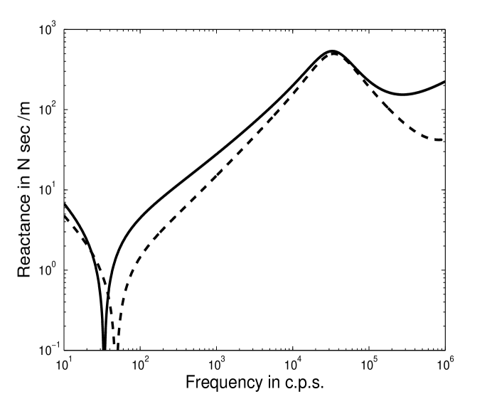
Figure 1: The reactance (real part of $Z$) for an oscillating sphere in a tissue-like material [1]. The solid and dashed curves correspond to a bonded ($\chi=0$) and slipping ($\chi=1$) spherical interface, respectively. The reactance is positive (mass-like) except for frequency below 30 c.p.s. (50 c.p.s. for the dashed curve) where it is negative (stiffness-like).

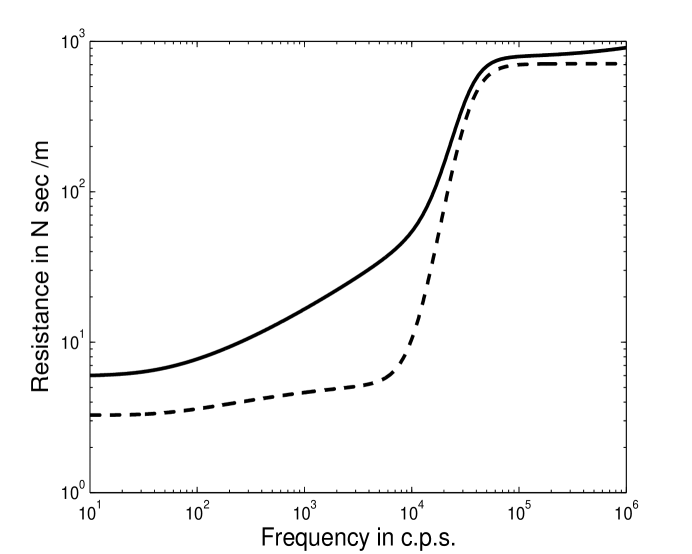
Figure 2: The resistance (imaginary part of $-Z$) for an oscillating sphere in a tissue-like material [1]. The solid and dashed curves correspond to a bonded ($\chi=0$) and slipping ($\chi=1$) spherical interface.