Voltage dependence of Landau-Lifshitz-Gilbert damping of a spin in a current driven tunnel junction

Abstract

We present a theory of Landau-Lifshitz-Gilbert damping $\alpha$ for a localized spin ${\vec{S}}$ in the junction coupled to the conduction electrons in both leads under an applied volatege $V$. We find the voltage dependence of the damping term reflecting the energy dependence of the density of states. We find the effect is linear in the voltage and cotrolled by particle-hole asymmetry of the leads.

I Introduction

Spintronics is an emerging subfield that holds the potential to replace conventional electronic devices with spintronic analogues where the manipulation, control, and readout of spins will enable novel functionality with no or little electronic charge dynamics spintronics . In order to realize this promise, the spin dynamics of the small scale devices needs to be well controlled. One of the most pressing questions concerns a set up which would preserve coherence and allow a manipulation of spins. In most systems, the relevant spin degrees of freedom are coupled to some bath, such as a fermionic bath of electrons. The detailed dynamics of single spins when in contact with such a bath plays a pivotal role in addressing decoherence in potential spintronic systems.

The conventional way to treat this problem is via a Caldeira-Leggett approach where the external bath is modeled by collective excitations which are capable of destroying coherent spin dynamics. Often, spin dynamics is described by a Landau-Lifshitz-Gilbert equation ll1 ; ll2 :

$${\frac{d{\vec{S}(t)}}{dt}}=-{\vec{S}(t)}\times{\vec{h}}-\alpha{\vec{S}(t)}\times{\frac{d{\vec{S}(t)}}{dt}},$$ (1)

where ${\vec{h}}$ is, up to constant prefactors, the external magnetic field and the coefficient $\alpha$ captures the damping due to the external bath. A caricature of the solution of this equation Chika is provided in Fig.1. There are standard methods to calculate $\alpha$ in an equilibrium situation when, say, one considers a spin in a Fermi liquid Heinrich ; Halperin .

In the current publication, we address a related novel question concerning the effect of an applied voltage bias on the Gilbert coefficient $\alpha$. Our work complements the recent results of Onoda wherein the effects of the “retarded” electronic contributions in the equations of motion for a system of spins were studied. Both such retarded correlations Zhu03 as well as additional “Keldysh” correlations generally manifest themselves in the single spin equations of motion, see e.g. nsabz for general spin equations of motion entailing the effects of both correlations. In the current work, we examine the voltage dependence of Gilbert damping. For the sake of clarity, we depart from the Keldysh contour formalism of Onoda ; Zhu03 ; nsabz , and use a Caldeira-Leggett approach.

In what follows, we consider the case of a junction between two electrodes that contains one spin $\vec{S}$, see Fig.2. This spin $\vec{S}$ may be the spin of a single magnetic impurity or it may portray the spin of a cluster at low temperature when the spins in the cluster are locked. Upon applying a finite bias between the electrodes of Fig.1, a current flow is generated. Thereafter, at long times, the system is at a steady but non-equilibrium state so long as the voltage bias $V$ is applied. We will focus on the voltage dependence of the damping term $\alpha(V)$ in Eq.(1). We find that the change in the density of states associated with the chemical potential gradient across the junction triggers a modification to the damping $\alpha$ that is linear in voltage and is proportional to the particle-hole assymmetry of the density of states. The scale of the correction is set by the Fermi energy of the metal in the leads $E_{F}$ and by particle-hole asymmetry in the density of states:

$$\alpha(V)=\alpha_{0}+\alpha_{1}(V)=\alpha_{0}(1+O(1)eV/E_{F}).$$ (2)

This result vividly illustrates the presence of voltage induced damping in such junctions. Spin unpolarized electrons tunneling across the junction interact via exchange interaction with the spin $\vec{S}$ and produce random magnetic fields that disorder the local spin. This noise augments that already present equilibrium magnetic noise in a Fermi liquid bath. Such a behavior of $\alpha(V)$ with the external voltage is in line with the works of hooley . An analysis of a related single spin problem in a Josephson junction (instead of the normal junction studied here) was advanced in Zhu03 ; nsabz ; bulaevskii .

We will shortly derive the effective single spin action from which the principle equation of motion of Eq.(1) follows. Several technical details of our derivation are given in the appendices.

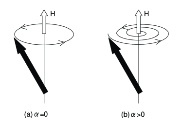
Figure 1: Sketch of the dissipative spin dynamics. Panel (a) depicts a cartoon of the Larmor precession of the spin about the direction of an applied magnetic field (B). In panel (b), a caricature of the spin dynamics in the presence of Landau-Lifshitz-Gilbert damping is shown.

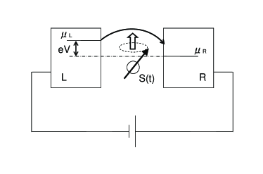
Figure 2: Magnetic impurity coupled to two electrodes. $\mu_{\rm L}$ and $\mu_{\rm R}$ denotes the chemical potentials of the left and right leads respectively. The voltage drop across the two electrodes is $eV=\mu_{L}-\mu_{R}$.

II THE SYSTEM AND OUR PRINCIPLE RESULTS

The physical system under consideration in this publication is illustrated in Fig.2. It consists of two (left(L) and right(R)) electrodes across which a voltage bias is applied; a magnetic impurity ($\vec{S}$) is situated in between (or lies on one of) the electrodes. An external magnetic field ${\vec{B}}$ is present. In the absence of effects stemming from conduction electrons in the tunneling barrier, the single spin would precess at the Larmor precession frequency about the applied field direction (see, e.g. panel (a) of Fig.1). With the external circuit elements present, the spin motion becomes dissipative (as schematically shown in panel (b) of Fig.1).

With the spin embedded in the tunneling barrier, the work function is modified and the conduction electron tunneling matrix element is supplanted by a Kondo like exchange term $J(\vec{S}\cdot\vec{\sigma}_{c})$, with $\vec{\sigma}_{c}$ denoting the conduction electron spin. In what follows, we will dispense with the $c$ subscript. The Hamiltonian governing this system is given by

$${\cal H} = {\cal H}_{e}+{\cal H}_{s}+{\cal H}_{T},$$ (3)

$${\cal H}_{e} = \sum_{\alpha,k,\sigma}\xi_{\alpha k}c_{\alpha k\sigma}^{\dagger}c_{\alpha k\sigma},$$

$${\cal H}_{s} = -{\vec{h}}\cdot{\vec{S}(t)},$$

$${\cal H}_{T} = {\frac{1}{\Omega}}{\sum_{\alpha,k,\sigma}}{\sum_{\beta,p,\sigma^{\prime}}}c_{\alpha k\sigma}^{\dagger}(T_{\alpha\beta})_{\sigma\sigma^{\prime}}c_{\beta p\sigma^{\prime}},$$ (4)

where $c_{\alpha k\sigma}^{\dagger}~{}(c_{\alpha k\sigma})$ creates (annihilates) an electron with momentum $k$ and spin $\sigma\in\{\uparrow,\downarrow\}$ in the lead $\alpha\in\{{\rm L},{\rm R}\}$. The abbreviation $\xi_{\alpha k}=\epsilon_{\alpha k}-\mu_{\alpha}$, where $\epsilon_{\alpha k}$ is the energy of electron with momentum $k$ in (the lead) $\alpha$ and $\mu_{\alpha}$ is the chemical potential in (the lead) $\alpha$. The second term in Eq.(4), ${\cal H}_{s}$, is Zeeman energy of the spin in an external magnetic field $\vec{B}$. Here, $\vec{h}\equiv g\mu_{B}{\vec{B}}$ with $g$ gyromagnetic ratio and $\mu_{B}$ the Bohr magneton. The last term in Eq.(4), ${\cal H}_{T}$, represents both Kondo coupling and direct tunneling process, where the amplitudes $\{T_{\alpha\beta}\}=\{T_{{\rm L}{\rm L}},T_{{\rm L}{\rm R}},T_{{\rm R}{\rm L}},T_{{\rm R}{\rm R}}\}$ are tunneling matrix elements and their explicit forms are

$$T_{LL} = J_{LL}({\vec{\sigma}}\cdot{\vec{S}(t)}),$$

$$T_{RR} = J_{RR}({\vec{\sigma}}\cdot{\vec{S}(t)}),$$

$$T_{LR} = T_{RL}=(T_{0}\delta_{\sigma\sigma^{\prime}}+J_{LR}({\vec{\sigma}}\cdot{\vec{S}(t)})).$$ (5)

Here, $T_{0}$ is the direct tunneling matrix element and $J_{\alpha\beta}$ is the Kondo coupling, ’while $\Omega$ denotes the Volume of each lead (assumed, for simplicity, to be the same)’. Typically, from the expansion of the work function for tunneling, ${J_{LR}}/{T_{0}}\sim J/U$, where $U$ is the height of a spin-independent tunneling barrier and $J$ the magnitude of the spin exchange interaction  Zhu_Balatsky . Typical values of the ratio the spin dependent to spin independent tunneling amplitudes in Eq.(5), $J_{\alpha\beta}/T_{0}$, are ${\cal{O}}(10^{-1})$, with a typical Fermi energy $E_{F}^{R}$ of the order of several electron-volts. From the Hermiticity of the Hamiltonian, we can find that the matrix element $(T_{\alpha\beta})_{\sigma\sigma^{\prime}}$ satisfies $((T_{\alpha\beta})_{\sigma\sigma^{\prime}})*=(T_{\beta\alpha})_{\sigma^{\prime}\sigma}.$

In the up and coming, we derive the effective action for the single impurity spin via an imaginary time path integral formalism. The full action is given by

$$S=\int_{0}^{\beta}d{\tau}\sum_{\alpha k\sigma}c_{\alpha k\sigma}^{\dagger}\partial_{\tau}c_{\alpha k\sigma}+iS\omega(\vec{S}(\tau))+\int_{0}^{\beta}d{\tau}{\cal H}(\tau),$$ (6)

where the second, Wess-Zumino-Novikov-Witten(WZNW), term in Eq.(6) depicts the Berry phase accumulated by the spin Fradkin . In our action, we have the following quadratic form of fermions,

$$\int_{0}^{\beta}d{\tau}{\frac{1}{\Omega}}\sum_{\alpha k\sigma}\sum_{\beta p\sigma^{\prime}}c_{\alpha k\sigma}^{\dagger}(\delta_{\alpha\beta}\delta_{\sigma\sigma^{\prime}}(\partial_{\tau}+\xi_{\alpha k})+(T_{\alpha\beta})_{\sigma\sigma^{\prime}})c_{\beta p\sigma^{\prime}}$$

$$\equiv\int_{0}^{\beta}d{\tau}{\frac{1}{\Omega}}\sum_{\alpha k\sigma}\sum_{\beta p\sigma^{\prime}}c_{\alpha k\sigma}^{\dagger}((M_{\alpha\beta}(\tau))_{\sigma\sigma^{\prime}})_{kp}~{}c_{\beta p\sigma^{\prime}}.$$ (7)

We may integrate over the lead electrons to obtain the effective action for the spin

$$S_{\rm{eff}}(\vec{S}(\tau))\sim iS\omega({\vec{S}(\tau)})+\int_{0}^{\beta}d{\tau}{\vec{h}}\cdot{\vec{S}(\tau)}-{\rm{ln}}{\rm{det}}M,$$ (8)

where ${\rm{det}}M$ means functional determinant of $M.$ From the third term in Eq.(8), we obtain a quadratic non-local in time interaction of the spin with itself, $\vec{S}(\tau)$ as

$$\Delta S(\vec{S}(\tau))=-2\int d{\tau}\int d{\tau^{\prime}}{\vec{S}(\tau)}\cdot{\vec{S}(\tau^{\prime})}K(\tau-\tau^{\prime}),$$ (9)

where

$$K(\tau) = \sum_{\alpha,\beta\in\{\rm{L,R}\}}K_{\alpha\beta}(\tau),$$

$$K_{\alpha\beta} = \sum_{k\in\alpha}\sum_{p\in\beta}{\frac{J_{\alpha\beta}J_{\beta\alpha}}{2}}{\frac{1}{\beta}}\sum_{\omega_{m}}{\frac{f(\xi_{k})-f(\xi_{p})}{i\omega_{m}+\xi_{k}-\xi_{p}}}e^{-i\omega_{m}\tau},$$ (10)

with $f(\xi)$ denotes the Fermi distribution function (see APPENDIX A). The effective action $\Delta S$ of Eq.(8) can be decomposed into two (trivial and non-trivial) components as $\Delta S=\Delta S_{\rm loc}+\Delta S_{\rm{dis}}$, with

$$\Delta S_{\rm loc} = -2K(\omega=0)\int d{\tau}({\vec{S}(\tau)})^{2},$$

$$\Delta S_{\rm{dis}} = \int d{\tau}\int d{\tau}^{\prime}({\vec{S}(\tau)}-{\vec{S}({\tau})})^{2}K(\tau-{\tau}^{\prime}).$$ (11)

Here, $K(\omega=0)$ is the zero-frequency Fourier component of $K(\tau)$. The first term ($\Delta S_{\rm loc}$) is a trivial constant as $S(\tau)^{2}=S^{2}$. The nonlocal part ($\Delta S_{\rm{dis}}$) represents the dissipative effect due to the coupling between $S(\tau)$ and electrons bath. The integral kernel $K(\tau)$ is calculated in the same way as the Caldeira-Leggett theory Leggett ; Leggett2 leading to

$$K(\tau)=\int_{0}^{\infty}d{\omega}J(\omega)\frac{{\rm cosh}({{\beta}/2}-|\tau|){\omega}}{{\rm sinh}({\beta\omega}/2)},$$ (12)

where $J(\omega)$ is the spectral density and its explicit form is

$$J(\omega)=\sum_{\alpha\beta}\sum_{k\in\alpha}\sum_{p\in\beta}{\frac{J_{\alpha\beta}J_{\beta\alpha}}{2}}[f(\xi_{k})-f(\xi_{p})]\delta(\omega+\xi_{k}-\xi_{p}).$$ (13)

The details of the derivation of Eq.(13) are provided in APPENDIX B. The spectral density of Eq.(13), $J(\omega)$, is estimated as

$$J(\omega) = \sum_{\alpha\beta}{\frac{J_{\alpha\beta}J_{\beta\alpha}}{2}}\int_{E_{F}^{\alpha}}^{\infty}d{\xi_{\alpha}}N(\xi_{\alpha})\int_{E_{F}^{\beta}}^{\infty}d{\xi_{\beta}}N(\xi_{\beta})$$ (14)

$$\times[f(\xi_{\alpha})-f(\xi_{\beta})]\delta(\omega-\xi_{\alpha}-\xi_{\beta})$$

$$\sim \sum_{\alpha\beta}{\frac{J_{\alpha\beta}J_{\beta\alpha}}{2}}N(\xi_{\alpha}=0)N(\xi_{\beta}=0)\omega,$$

where $E_{F}^{\alpha}$ denotes the Fermi Energy of the lead $\alpha$. It is obvious that $J(\omega)$ in Eq.(14) is proportional to $\omega$, i.e., $J(\omega)$ is Ohmic. If spectral density is expressed as $J(\omega)={\eta\omega}/{2\pi}$, then the Gilbert coefficient $\alpha$ in Eq.(1) is exactly equal to $\eta$. By varying the total action with respect to the spin ${\delta S}/{\delta{\vec{S}(\tau)}}=0$, we immediately obtain the Landau-Lifshitz-Gilbert equation with $\alpha={\frac{2\pi}{\omega}}J(\omega)$(see APPENDIX C). In other words, the voltage dependence of $\alpha$ in Eq.(1) is identically the same as that of $J(\omega)$. We next examine the voltage dependence of $J(\omega)$.

If we apply a voltage leading to a chemical drop of $\Delta\mu_{L}-\Delta\mu_{R}=eV$. Assuming, for example,that the net charge on both right and left leads is unchanged, we also have $D^{L}(E_{F})\Delta\mu_{L}+D^{R}(E_{F})\Delta\mu_{R}=0$. With these constraints we get

$$\Delta\mu_{L} = \frac{D^{R}(E_{F})}{D^{L}(E_{F})+D^{R}(E_{F})}eV,$$

$$\Delta\mu_{R} = -\frac{D^{L}(E_{F})}{D^{L}(E_{F})+D^{R}(E_{F})}eV,$$ (15)

the Gilbert coefficient $\alpha$ may be approximated as

$$\alpha(V) \sim 2\pi\Bigl{(}\frac{J_{LL}^{2}}{2}D^{L}(E_{F}+\Delta\mu_{L})^{2}+\frac{J_{RR}^{2}}{2}D^{R}(E_{F}+\Delta\mu_{R})^{2}$$

$$+J_{LR}^{2}D^{L}(E_{F}+\Delta\mu_{L})D^{R}(E_{F}+\Delta\mu_{R})\Bigr{)}$$

$$\sim 2\pi\Bigl{(}\frac{[J_{LL}D^{L}(E_{F})]^{2}}{2}+\frac{[J_{RR}D^{R}(E_{F})]^{2}}{2}+J^{2}_{LR}D^{L}(E_{F})D^{R}(E_{F})$$

$$+(J^{2}_{LL}D^{L}(E_{F})\frac{\partial{D^{L}(E_{F})}}{\partial{E_{F}}}+J^{2}_{LR}D^{R}(E_{F})\frac{\partial{D^{L}(E_{F})}}{\partial{E_{F}})})\Delta\mu_{L}$$

$$+(J^{2}_{RR}D^{R}(E_{F})\frac{\partial{D^{R}(E_{F})}}{\partial{E_{F}}}+J^{2}_{LR}D^{L}(E_{F})\frac{\partial{D^{R}(E_{F})}}{\partial{E_{F}})})\Delta\mu_{R})\Bigr{)}$$

$$= 2\pi\Bigl{(}\frac{[J_{LL}D^{L}(E_{F})]^{2}}{2}+\frac{[J_{RR}D^{R}(E_{F})]^{2}}{2}+J^{2}_{LR}D^{L}(E_{F})D^{R}(E_{F})$$ (16)

$$+ \frac{eV}{D^{L}(E_{F})+D^{R}(E_{F})}(J^{2}_{LL}D^{L}(E_{F})D^{R}(E_{F})\frac{\partial{D^{L}(E_{F})}}{\partial{E_{F}}}$$

$$- J^{2}_{RR}D^{L}(E_{F})D^{R}(E_{F})\frac{\partial{D^{R}(E_{F})}}{\partial{E_{F}}}$$

$$+ J^{2}_{LR}D^{R}(E_{F})D^{R}(E_{F})\frac{\partial{D^{L}(E_{F})}}{\partial{E_{F}}}$$

$$- J^{2}_{LR}D^{L}(E_{F})D^{L}(E_{F})\frac{\partial{D^{R}(E_{F})}}{\partial{E_{F}}})\Bigr{)}.$$

The change in the density of states associated with the chemical potential gradient across the junction triggers a modification of the damping $\alpha$ that is linear in voltage. For typical Fermi energy $E_{F}^{L/R}$ of the order of several electron-volts, the voltage dependence of $\alpha$ may become very notable. This voltage driven effect may be expressed in terms of $\alpha_{0}$ and $\alpha_{1}(V)$ with $\alpha(V)=\alpha_{0}+\alpha_{1}$ (Eq.(2)). Here

$$\alpha_{0}=\pi\bigl{(}J_{LL}^{2}[D(E_{F}^{L})]^{2}+2J_{LR}^{2}D(E_{F}^{L})D(E_{F}^{R})+J_{RR}^{2}[D(E_{F}^{R})]^{2}\bigl{)},$$

$$\alpha_{1}=\frac{1}{4e|T_{0}|^{2}[D(E_{F}^{L})+D(E_{F}^{R})]}\Bigl{(}\frac{I_{o}^{L}}{[D(E_{F}^{L})]^{2}}+\frac{I_{o}^{R}}{[D(E_{F}^{R})]^{2}}\Bigl{)}$$

$$\times\bigl{[}D(E_{F}^{L})D(E_{F}^{R})\bigl{(}J_{LL}^{2}\frac{\partial D^{L}(E_{F})}{\partial E_{F}}-J_{RR}^{2}\frac{\partial D^{R}(E_{F})}{\partial E_{F}}\bigl{)}$$

$$+J_{LR}^{2}\bigl{(}[D(E_{F}^{R})]^{2}\frac{\partial D^{L}(E_{F})}{\partial E_{F}}-[D(E_{F}^{L})]^{2}\frac{\partial D^{R}(E_{F})}{\partial E_{F}}\bigl{)}\bigl{]}.$$ (17)

III Conclusions

In conclusion, we present a theoretical study of Landau-Lifshitz-Gilbert damping (Eq.(1)) for a localized spin ${\vec{S}}$ in a junction. The exchange interactions between the localized spin and tunneling electrons leads to additional dissipation of the spin motion, see Fig.(1). In the presence of an applied voltage bias $V$, the damping coefficient, i.e., Gilbert damping, is modified in linear order in $V$ for the leads with particle-hole asymmetry in the Density of States.

IV Acknowledgements

Work at LANL was supported by the US DOE under LDRD X1WX.

V Appendix A: DERIVATION OF THE EFFECTIVE ACTION

Here we will give a detailed derivation of the effective action for a spin. From Eq.(8), we can extract a quadratic form of spins with the aid of the well known identity ${\rm{ln}}~{}{\rm{det}}M={\rm Tr}~{}{\rm{ln}}M.$ In order to tabulate the expansion of ${\rm Tr}~{}{\rm{ln}}M$ perturbatively, we define matrices $M_{0}$ and $M_{1}$,

$$M_{KP} =(M_{0})_{KP}+(M_{1})_{KP}$$

$$(M_{0})_{KP} \equiv((-i\omega+\xi_{\alpha k})\delta_{\alpha\beta}\delta_{\sigma\sigma^{\prime}})\delta_{KP}$$

$$(M_{1})_{KP} \equiv{\frac{1}{\sqrt{\beta}}}(T_{\alpha\beta}(\omega-\omega^{\prime}))_{\sigma\sigma^{\prime}},$$

where $K\equiv(k,\omega)$ and $P\equiv(p,\omega^{\prime})$ with fermionic Matsubara frequencies $\omega$ and $\omega^{\prime}$. Employing the expansion ${\rm ln}(1+x)=-\sum_{n=1}^{\infty}{\frac{(-x)^{n}}{n}}$, we can write the effective action as

$$S_{\rm{eff}}(\vec{S}(\tau))\sim S_{0}+{\rm{Tr}}~{}{\rm{ln}}M_{0}+{\rm{Tr}}(M_{0}^{-1}M_{1})-{\frac{1}{2}}{\rm{Tr}}(M_{0}^{-1}M_{1})^{2}+\cdots,$$ (18)

where $S_{0}$ is the sum of the first and the second term in Eq.(8). The third term in Eq.(8) (and consequent last term shown in Eq.(18)) is the first non-trivial contribution to the spin equation of motion. Its evaluation is straightforward,

$${\rm Tr}(M_{0}^{-1}M_{1})^{2}$$

$$=\sum(M_{0}^{-1})_{K_{1}K_{1}}(M_{1})_{K_{1}K_{2}}(M_{0}^{-1})_{K_{2}K_{2}}(M_{1})_{K_{2}K_{1}}$$

$$={\frac{1}{2\beta}}\sum(-i\omega+\xi_{\alpha k})^{-1}(T_{\alpha\beta}(\omega-\omega^{\prime}))_{\sigma\sigma^{\prime}}$$

$$(-i\omega^{\prime}+\xi_{\beta p})^{-1}(T_{\beta\alpha}(\omega^{\prime}-\omega))_{\sigma^{\prime}\sigma},$$

where, repeated indices are implicitly summed over. Then, we find

$$\Delta S={\frac{1}{2}}{\rm Tr}(M_{0}^{-1}M_{1})^{2}$$

$$={\frac{1}{2\beta}}\sum_{\omega\omega^{\prime}}\sum_{\alpha\beta}\sum_{\sigma\sigma^{\prime}}\sum_{k\in\alpha}\sum_{p\in\beta}(-i\omega+\xi_{\alpha k})^{-1}(T_{\alpha\beta}(\omega-\omega^{\prime}))_{\sigma\sigma^{\prime}}$$

$$(-i\omega^{\prime}+\xi_{\beta p})^{-1}(T_{\beta\alpha}(\omega^{\prime}-\omega))_{\sigma^{\prime}\sigma}$$

$$=-\sum_{\alpha\beta}\sum_{k\in\alpha}\sum_{p\in\beta}\sum_{\omega_{m}}J_{\alpha\beta}J_{\beta\alpha}{\frac{f(\xi_{k})-f(\xi_{p})}{i\omega_{m}+\xi_{k}-\xi_{p}}}{\vec{S}}(-\omega_{m})\cdot{\vec{S}}(\omega_{m})$$

$$\equiv-\int d\tau\int d\tau^{\prime}{\vec{S}}(\tau)\cdot{\vec{S}}(\tau^{\prime})2K(\tau-\tau^{\prime}).$$

Here, $K(\tau-\tau^{\prime})$ denotes the integral kernel defined in Eq.(10). Upon invoking the identity $2{\vec{S}(\tau)}\cdot{\vec{S}({\tau}^{\prime})}=(({\vec{S}(\tau)})^{2}+({\vec{S}({\tau}^{\prime})})^{2})-({\vec{S}(\tau)}-{\vec{S}({\tau}^{\prime})})^{2}$, the effective action becomes that of Eq.(11).

VI APPENDIX B: THE DERIVATION OF THE SPECTRAL DENSITY

We return to Eq.(10) derived in Appendix A, and express the sum as a contour integral following standard procedures, e.g.Mahan , to obtain

$$K_{\alpha\beta} = {\frac{J_{\alpha\beta}J_{\beta\alpha}}{2}}\sum_{k\in\alpha}\sum_{p\in\beta}\oint{\frac{dz}{2\pi i}}\Bigl{(}{\frac{e^{-z\tau}}{e^{\beta z}-1}}\theta(-\tau)+{\frac{e^{-z\tau}}{1-e^{-\beta z}}}\theta(\tau)\Bigr{)}{\frac{f(\xi_{k})-f(\xi_{p})}{z+\xi_{k}-\xi_{p}}}$$ (19)

$$= P\int_{-\infty}^{\infty}d{\omega}\Bigl{(}{\frac{J_{\alpha\beta}J_{\beta\alpha}}{2}}\Bigr{)}\sum_{k\in\alpha}\sum_{p\in\beta}[f(\xi_{k})-f(\xi_{p})]\delta(\omega+\xi_{k}-\xi_{p})\Bigl{(}{\frac{e^{-\omega\tau}}{e^{\beta\omega}-1}}\theta(-\tau)+{\frac{e^{-\omega\tau}}{1-e^{-\beta\omega}}}\theta(\tau)\Bigr{)}$$

$$= P\int_{0}^{\infty}d{\omega}\Bigl{(}-{\frac{J_{\alpha\beta}J_{\beta\alpha}}{2}}\sum_{k\in\alpha}\sum_{p\in\beta}[f(\xi_{k})-f(\xi_{p})]\delta(\omega+\xi_{k}-\xi_{p})\Bigr{)}\frac{{\rm cosh}({{\beta}/2}-|\tau|){\omega}}{{\rm sinh}({\beta\omega}/2)}$$

$$\equiv \int_{0}^{\infty}d{\omega}J(\omega)\frac{{\rm cosh}({{\beta}/2}-|\tau|){\omega}}{{\rm sinh}({\beta\omega}/2)}$$

where $J(\omega)$ denotes the spectral density in Caldeira-Leggett theory. The standard contour employed here is shown in Fig.(3). The symbol $P$ in Eq.(19) denotes the principal part of the integral.

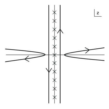
Figure 3: The standard contour employed in Eq.(19) in order to evaluate the Matsubara sum of Eq.(10). The crosses along the imaginary axis denote the Matsubara frequencies.

The spectral density $J(\omega)$ in Eq.(14)

$$J(\omega)=\frac{J_{LL}^{2}}{2}\int_{-E_{F}^{L}}^{\infty}d{\xi_{L}}N(\xi_{L})\int_{-E_{F}^{L}}^{\infty}d{\xi_{L}^{\prime}}N(\xi_{L}^{\prime})[f(\xi_{L})-f(\xi_{L}^{\prime})]\delta(\omega+{\xi_{L}}-{\xi_{L}^{\prime}})$$

$$+\frac{J_{RR}^{2}}{2}\int_{-E_{F}^{R}}^{\infty}d{\xi_{R}}N(\xi_{R})\int_{-E_{F}^{R}}^{\infty}d{\xi_{R}^{\prime}}N(\xi_{R}^{\prime})[f(\xi_{R})-f(\xi_{R}^{\prime})]\delta(\omega+{\xi_{R}}-{\xi_{R}^{\prime}})$$

$$+J_{LR}^{2}\int_{-E_{F}^{L}}^{\infty}d{\xi_{L}}N(\xi_{L})\int_{-E_{F}^{R}}^{\infty}d{\xi_{R}}N(\xi_{R})[f(\xi_{L})-f(\xi_{R})]\delta(\omega+{\xi_{L}}-{\xi_{R}})$$

$$\sim\Bigl{(}\frac{J_{LL}^{2}}{2}N(\xi_{L}=0)N(\xi_{L}^{\prime}=0)+\frac{J_{RR}^{2}}{2}N(\xi_{R}=0)N(\xi_{R}^{\prime}=0)+J_{LR}^{2}N(\xi_{L}=0)N(\xi_{R}=0)\Bigr{)}\omega$$

$$=\Bigl{(}\frac{J_{LL}^{2}}{2}D^{L}(E_{F}^{L})D^{L}(E_{F}^{L})+\frac{J_{RR}^{2}}{2}D^{R}(E_{F}^{R})D^{R}(E_{F}^{R})+J_{LR}^{2}D^{L}(E_{F}^{L})D^{R}(E_{F}^{R})\Bigr{)}\omega,$$ (20)

where $D^{L/R}(E^{L/R}_{F})$ denotes the density of states at the Fermi energy level of the left/right lead.
If we apply a voltage leading to a chemical potential drop of $E^{L}_{F}-E^{R}_{F}=(E_{F}+\Delta\mu_{L})-(E_{F}+\Delta\mu_{R})=eV$, then Eq.(13) follows. This, in turn, leads to Eq.(16). then Eq.(13) follows.

VII APPENDIX C: THE SPIN EQUATION OF MOTION

If $J(\omega)=\frac{\alpha\omega}{2\pi}$ then, from Eq.(12), the non-local in time kernel of the action (Eq.(9)) is $K(\tau)\sim{\frac{\alpha}{2\pi}}{\frac{1}{{\tau}^{2}}}$. We thus obtain from Eq.(11),

$$\Delta S_{dis}={\frac{\alpha}{2\pi}}\int d{\tau}\int d{\tau}^{\prime}{\frac{({\vec{S}(\tau)}-{\vec{S}({\tau}^{\prime})})^{2}}{(\tau-{\tau}^{\prime})^{2}}}.$$ (21)

The functional derivative of $\Delta S_{\rm{dis}}$ with respect to $\vec{S}(\tau)$ is

$${\frac{\delta\Delta S_{dis}}{\delta S(\tau)}}={\frac{\alpha}{\pi}}\int d{\tau}^{\prime}{\frac{({\vec{S}(\tau)}-{\vec{S}({\tau}^{\prime})})}{(\tau-{\tau}^{\prime})^{2}}}$$

$$={\frac{\alpha}{\pi}}\int d{\tau}^{\prime}{\frac{1}{(\tau-{\tau}^{\prime})}}{\frac{d}{d{\tau}^{\prime}}}({\vec{S}(\tau)}-{\vec{S}({\tau}^{\prime})})=i\alpha{\frac{d}{d{\tau}}}{\vec{S}(\tau)}$$ (22)

From the free portion of the action (the first two terms of Eq.(8)), we have

$${\frac{\delta S_{0}}{\delta{\vec{S}(\tau)}}}=i{\frac{1}{S^{2}}}{\frac{d{\vec{S}(\tau)}}{d{\tau}}}\times{\vec{S}(\tau)}+\vec{h}.$$ (23)

Adding Eqs.(22,23), equating the sum to zero, cross multiplying with $\vec{S}(\tau)$, and changing $\tau\to it$, we obtain Eq.(1).

References

• (1) D. D. Awschalom, M. E. Flatte, and N.Samarth, Spintronics, Scientific American, pp. 67-73, June 2002.
• (2) T. L. Gilbert, Phys. Rev. 100, 1243 (1955)
• (3) L. Landau and E. M. Lifshitz, Physik Zeits. Soviets. 8, 153 (1935)
• (4) S. Chikazumi, Physics of Ferromagnetism, (Oxford university press, Oxford, 1997)
• (5) B. Heinrich, D. Fraitová, and V. Kamberský, Phys. Status. Solidi, 23, 501 (1967).
• (6) Y. Tserkovnyak, G. A. Fiete and B. I. Halperin, Appl. Phys. Lett. 84, 5234 (2004).
• (7) M. Onoda and N. Nagaosa, cond-mat/0509058
• (8) Jian-Xin Zhu, Z. Nussinov, A. Shnirman and A. V. Balatsky, Phys. Rev. Lett., 92, 107001 (2004).
• (9) Z. Nussinov, A. Shnirman, D. P. Arovas, A. V. Balatsky, and J-X. Zhu, Phys. Rev. B 71, 214520 (2005)
• (10) O. Parcollet and C. Hooley, Phys. Rev. B 66, 085315 (2002); L. N. Bulaevskii, M. Hruska, and G. Ortiz, Phys. Rev. B 68, 125415 (2003)
• (11) L. Bulaevskii, M. Hruska, A. Shnirman, D. Smith, and Yu. Makhlin, Phys. Rev. Lett. 92, 177001 (2004)
• (12) J-X. Zhu, and A. V. Balatsky, Phys. Rev. B 67, 174505 (2003)
• (13) E. Fradkin, Field Theories of Condensed Matter Systems (Addison-Wesley, Redwood City, 1991).
• (14) A. O. Caldeira and A. J. Leggett, Ann. Phys, 149, 374(1983).
• (15) A. O. Caldeira and A. J. Leggett, Phys. Rev. Lett, 46, 211(1981).
• (16) G. D. Mahan, Many-Particle Physics (Kluwer, New York, 2000).