Simulations of Disordered Bosons on Hyper-Cubic Lattices

Abstract

We address computational issues relevant to the study of disordered quantum mechanical systems at very low temperatures. As an example we consider the disordered Bose-Hubbard model in three dimensions directly at the Bose-glass to superfluid phase transition. The universal aspects of the critical behaviour are captured by a (3 + 1) dimensional link-current model for which an efficient ‘worm’ algorithm is known. We present a calculation of the distribution of the superfluid stiffness over the disorder realizations, outline a number of important considerations for performing such estimates, and suggest a modification of the link-current Hamiltonian that improves the numerical efficiency of the averaging procedure without changing the universal properties of the model.

1 . Introduction

The Bose-Hubbard model was first studied in the context of liquid helium in a disordered medium [6]. Interest in the model has recently grown with the progress achieved in trapping ultra-cold atomic gases in optical lattice potentials. The model describes the competition between tunneling and on-site interactions in a lattice of bosons. It displays several zero-temperature quantum phases that are now clearly attainable in the laboratory [7]. Notably, a localized Mott insulating (MI) phase exists when the tunneling between sites is small, while at higher tunneling the system becomes a superfluid (SF). In the presence of disorder another localized phase, the Bose-glass (BG), exists between the Mott insulator and the superfluid. In the present study we focus on the Bose-glass to superfluid transition since it exists only at finite disorder and thus provides a clear example of a quantum phase transition for which disorder is relevant. Although this model has been extensively studied in one- and two-dimensions, the nature of the phase transition in three and higher dimensions has received relatively little attention.

Scaling theories based on generalized Josephson relations and the finite compressibility of the superfluid and Bose-glass phases indicate that the dynamic correlation exponent $z$ is equal to the number of spatial dimensions [6]. This feature, which is supported by analytical and numerical arguments [8, 9, 13] in low dimensions suggests that the model has an unusual approach to mean-field behaviour—and may not have an upper critical dimension at all—invalidating standard renormalization group approaches. Numerical work above two dimensions is difficult due to the large volumes of the systems, and the algorithmic slow down of the Monte Carlo averaging procedure.

Of particular interest are the distributions of thermodynamic observables over the disorder. They are typically far from Gaussian in nature, rendering standard estimates of statistical error invalid for smaller sample sizes and necessitating calculations for a large number of disorder configurations. Moreover, the behaviour of these distributions for increasing lattice size is directly relevant to the break-down of self-averaging [2], the quantum Harris Criterion [5, 11], and the effect of disorder on quantum critical phenomena [12]. More efficient ways of performing disorder averages has also been proposed [3]. These latter developments are however too computationally demanding for the present model.

The universal properties of the $d$-dimensional Bose-Hubbard model are captured by a ($d$ + 1)-dimensional classical link-current representation for which an efficient worm-like Monte Carlo algorithm exists. While the worm algorithm represents a drastic improvement over earlier, Metropolis-like algorithms, the computational demands increase dramatically in higher dimensions, limiting the precision of the numerical analysis. Since the system is disordered, the calculations involve performing many Monte Carlo simulations of the system at the same parameters with different realizations of the disorder. Hence, the calculations are very well suited for parallelization and a linear speed up can be achieved with a relatively modest programming effort. Without such a linear speed up the calculations we report on would have been almost impossible. Parallelization is performed straightforwardly with MPI: each processor performs Monte Carlo simulations serially for a given disorder realization, then the results are collected and written to disk. As many as several thousand disorder realizations need to be performed at each point in parameter space, and each individual Monte Carlo simulation can take up to three hours, depending on the system size and the parameters of the model. The length of time required to perform one simulation for a given disorder realization dictates how large a system we can reasonably study and so it is essential to consider carefully how much computational effort to invest in each such simulation.

Numerical study of this transition in three dimensions presented a number of difficulties in calculating the disorder distributions and their averages. The main results of the study will be presented elsewhere [10], but we outline here the procedure that was used to estimate these distributions, and suggest a modification to the link-current Hamiltonian which improves the efficiency of these numerical estimates. The remainder of the introduction discusses the link-current Hamiltonian and the finite-size scaling theory on which our numerical approach relies. Section 2 describes how we ensure that the simulation of each disorder realization has been properly equilibrated. Section 3 describes a modification of the link-current model that improves the numerical efficiency of each simulation without affecting the universal details. We then conclude with some remarks about the general applicability of these considerations.

1.1 . Model and Scaling Theory

The Bose-Hubbard Hamiltonian, including an on-site disorder in the chemical potential is [6]

$$H_{\mathrm{BH}}=\sum_{{\bf r}}\Big{[}\frac{U}{2}\hat{n}_{{\bf r}}(\hat{n}_{{\bf r}}-1)-\mu_{{\bf r}}\hat{n}_{{\bf r}}\Big{]}-\frac{t}{2}\sum_{\langle{\bf r},{\bf r}^{\prime}\rangle}(\bm{\hat{\Phi}^{\dagger}_{r}\hat{\Phi}_{r^{\prime}}}+\mathrm{H.c.}).$$ (1)

The second quantized boson operators describe a tunneling process coupled by $t$ and an on-site, repulsive interaction $U$, on a hyper-cubic lattice. The disordered chemical potential $\mu_{\bf r}$ is distributed uniformly on $[\mu-\Delta,\mu+\Delta]$ so that $\Delta$ controls the strength of the disorder. At finite disorder, the system undergoes a phase transition from a Bose-glass insulating phase (low $t$, high $U$) to a superfluid phase (high $t$, low $U$). The model can be transformed via the quantum rotor model to the ($d$ + 1) link-current model [13]. The link-current Hamiltonian is given by

$$H=\frac{1}{K}\sum_{({\bf r},\tau)}\Big{[}\frac{1}{2}\bm{J}^{2}_{({\bf r},\tau)}-\mu_{{\bf r}}J^{\tau}_{({\bf r},\tau)}\Big{]}.$$ (2)

The integer currents ${\bf J}_{({\bf r},\tau)}$ are situated on the bonds of the lattice and obey a divergenceless constraint

$$\sum_{\nu=x,y,z,\tau}J^{\nu}_{({\bf r},\tau)}=0.$$ (3)

The resulting loops are interpreted as currents of bosons hopping about on the lattice (specifically they are fluctuations from an average density, so that the currents are permitted to be negative). The coupling $K$ controls the ratio between $t$ and $U$: at low $K$ the interaction $U$ dominates and the system is insulating, while at high $K$ the tunneling dominates and the system condenses into a superfluid.

The two phases can be distinguished by the superfluid stiffness, $\rho$, which is proportional to the superfluid density. The stiffness is defined as the response of the free energy to a twist in the boundary conditions and is indicative of global phase coherence. In the link-current model, the stiffness is proportional to the square of the winding number in the spatial dimensions:

$$\rho=\frac{1}{L^{d-2}L_{\tau}}\big{[}\langle n_{x}^{2}\rangle\big{]}_{av}.$$ (4)

The angle brackets $\langle\cdot\rangle$ denote a thermal average, while the square brackets $[\cdot]_{av}$ denote an average over disorder realizations. The winding numbers ($n_{\gamma}=L_{\gamma}^{-1}\sum_{{\bf r},\tau}J^{\gamma}_{{\bf r},\tau}$ for $\gamma=x,y,z,\tau$) of the lattice in each direction are just the number of current loops that have wound all the way about the periodic lattice. They are always integers.

Dynamics and statics are both essential to the critical behaviour of quantum phase transitions. They are characterized by independent spatial and temporal correlation lengths ($\xi$ and $\xi_{\tau}$) which define the dynamic critical exponent $z$:

$$\xi_{\tau}\sim\xi^{z}\sim(\delta^{-\nu})^{z},\qquad\delta=\frac{K-K_{c}}{K_{c}}.$$ (5)

Here $\nu$ is the correlation length exponent. This implies that quantities at the critical point scale as a function of two arguments. The superfluid stiffness (which diverges as $\rho\sim\xi^{d+z-2}$ at $K_{c}$) thus scales as

$$\rho=\frac{1}{L^{d+z-2}}\bar{\rho}(L^{1/\nu}\delta,L_{\tau}/L^{z}).$$ (6)

If we hold the second argument constant, the critical point can be located by plotting curves of $\rho L^{d+z-2}$ for various linear system sizes $L$. Since $\delta=0$ at $K_{c}$, $K_{c}$ will be the value of $K$ at which these curves intersect. This unfortunately requires that we guess at the value of $z$ before we begin. In principle, we are free to set the aspect ratio

$$\alpha=L_{\tau}/L^{z},$$ (7)

as we see fit to find the critical point; in practice however, as we discuss below, the numerics work better near an optimal aspect ratio where $(\xi/L)^{z}\simeq\xi_{\tau}/L_{\tau}$ implying $\alpha={\cal O}(1)$.

2 . Equilibration

When considering disordered systems, the average $[\langle\cdot\rangle]_{av}$ of an arbitrary observable (denoted by $\cdot$) such as the stiffness $\rho$ must be calculated over a whole set of disorder configurations, performing independent Monte Carlo simulations on each particular realization. We must then decide how many Monte Carlo sweeps ($t_{n}$) to perform on each simulation, and how many disorder realizations ($N_{D}$) to average these over. There are correspondingly two sources of statistical error [4]: the error $\delta_{T}\rho$ in the estimate of the thermal average:

$$\langle\rho\rangle=\bar{\rho}+\delta_{T}\rho,$$ (8)

and the overall error $\delta[\rho]_{av}$ in the disorder average:

$$[\langle\rho\rangle]_{av}=[\bar{\rho}+\delta_{T}\rho]_{a}v=[\bar{\rho}]_{av}+\delta[\rho]_{av}.$$ (9)

It is of particular interest to review [4] how to correctly obtains the disorder average of the square of a thermodynamic observable such as the energy. Such a quantity would be needed for calculating for instance the specific heat, $C_{V}$. In this case we have for a single disorder realization:

$$\langle E\rangle=\bar{E}+\delta_{T}E.$$ (10)

If we now want to calculate the disorder average $[\langle E\rangle^{2}]_{av}$ we encounter a slight problem:

$$[\langle E\rangle^{2}]_{av}=[\bar{E}^{2}]_{av}+[(\delta_{T}E)^{2}]_{av}+2\bar{E}[\delta_{T}E]_{av}.$$ (11)

It is natural to assume that $[\delta_{T}E]_{av}$ will yield zero when a sufficiently large number of disorder realizations are used. However, $[(\delta_{T}E)^{2}]_{av}$ will be non zero and will yield a systematic error unless infinitely precise thermal averages can be obtained for each disorder realization. In order to circumvent this problem and correctly calculate such a disorder average, one can run 2 independent simulations, referred to as “replicas”, of a given disorder realization [4]. We denote them by $\alpha$ and $\beta$. The above disorder average should then be calculated in the following way:

$$[\langle E\rangle^{2}]_{av} \equiv [\langle E^{\alpha}\rangle\langle E^{\beta}\rangle]_{av}$$ (12)

$$= [\bar{E}^{2}]_{av}+[\delta_{T}E^{\alpha}\delta_{T}E^{\beta}]_{av}$$

$$+\bar{E}[\delta_{T}E^{\alpha}]_{av}+\bar{E}[\delta_{T}E^{\beta}]_{av}.$$

The term $[\delta_{T}E^{\alpha}\delta_{T}E^{\beta}]_{av}$ will now also correctly average to zero since the thermal errors from each replica are independent random variables. In our calculations we always run at least two independent replicas of a given disorder realization with the goal of correctly calculating averages as outlined above. For higher powers of thermal averages more replicas are needed. As we shall see below, having several independent runs of a given disorder realization allow also for very convenient and indispensable checks of the equilibration of the calculations.

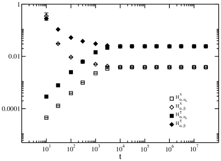
Figure 1: Hamming distances on an 8x8x8x64 lattice at ${\bf K_{c}=0.19}$ calculated over a set of 1000 disorder realizations with ${\bf t_{0}=3\times 10^{7}}$. For the Hamming distances between the two replicas ${\bf\alpha}$ and ${\bf\beta}$, ${\bf t}$ is the total number of Monte Carlo sweeps performed. For the Hamming distances between replica ${\bf\alpha}$ and its configuration ${\bf\alpha_{0}}$ at ${\bf t_{0}}$, ${\bf t}$ is the number of sweeps performed after the initial ${\bf t_{0}}$ sweeps have been performed. The convergence of the curves indicates ${\bf t_{r}\approx 3\times 10^{5}}$.

It is important to note that even for very large system sizes, the average should be taken over as many disorder realizations as possible. One might assume that for large system sizes a smaller set of disorder realizations would suffice, since the properties of the system will average out spatially. For many disordered systems this assumption is false—self-averaging breaks down [1]. Even in the thermodynamic limit (where in principle one could find any particular finite disorder realization somewhere in the infinite system) the width of the distribution of $P(\bar{\rho})$ remains finite. Moreover, such distributions are typically far from Gaussian (they often have a particularly ‘fat’ tail). Error estimates based on Gaussian distributions are thus only valid for very large $N_{D}$. The best approach is then to spend a minimal amount of computational time on each realization, and then rely on the disorder average to control the statistical errors. As usual, however, each Monte Carlo simulation must be properly equilibrated to ensure that $\langle\rho\rangle$ is unbiased. Since the lattice starts in an artificial (and non-equilibrium) configuration, we throw out the first $t_{0}$ of the $t_{n}$ sweeps before sampling the remaining $t_{s}=t_{n}-t_{0}$ configurations. As long as $t_{0}$ is greater than the relaxation time of the algorithm $t_{r}$, we sample only equilibrium configurations, and our estimates of the thermal averages will be unbiased. Since we do not want to spend all of our computational efforts equilibrating systems, each disorder realization is typically run for an additional $t_{0}$ steps once it has reached equilibrium.

To confirm that we have chosen $t_{0}$ greater than $t_{r}$, we perform each simulation independently on two replicas with different initial configurations. We can then define ‘Hamming distances’ [13] between the two replicas $\alpha$ and $\beta$ after performing $t$ Monte Carlo sweeps on their initial configuration, and between the replica $\alpha$ at sweep $t+t_{0}$ and its configuration $\alpha_{0}$ at sweep $t_{0}$ when sampling begins:

$$H_{\alpha,\alpha_{0}}^{\nu=x,\tau}(t)=\frac{1}{L^{d}L_{\tau}}\sum_{({\bf r},\tau)}\big{[}J^{\nu}_{\alpha:({\bf r},\tau)}(t+t_{0})-J^{\nu}_{\alpha:({\bf r},\tau)}(t_{0})\big{]}^{2},$$

$$H_{\alpha,\beta}^{\nu=x,\tau}(t)=\frac{1}{L^{d}L_{\tau}}\sum_{({\bf r},\tau)}\big{[}J^{\nu}_{\alpha:({\bf r},\tau)}(t)-J^{\nu}_{\beta:({\bf r},\tau)}(t)\big{]}^{2}.$$ (13)

These measures are then averaged over the disorder realizations. At the beginning of each simulation, the initial configurations of $\alpha$ and $\beta$ are quite different. Hence $H_{\alpha,\beta}(t)$ will be large for small $t$, but diminish as the two configurations equilibrate. On the other hand, shortly after $t_{0}$, the configuration $\alpha$ will not have changed substantially from $\alpha_{0}$, so $H_{\alpha,\alpha_{0}}(t)$ will be initially small, but increase as more sweeps are performed. If $t_{0}$ has in fact been chosen greater than $t_{r}$, these two measures will converge on the same value in $t_{r}$ sweeps at which point the configurations of $\alpha$, $\alpha_{0}$, and $\beta$ will be independently drawn from the same population of equilibrium configurations. Figure 1 shows the two Hamming distances plotted as a function of $t$ at $K_{c}$, averaged over $N_{D}=1000$ disorder realizations. Results are shown for Hamming distances defined in terms of spatial ($x,y,z$) currents (open symbols) and the temporal ($\tau$) current (filled symbols). Both the spatial and temporal Hamming distances converge, indicating that $t_{r}\approx 3\times 10^{5}$ for an 8x8x8x64 lattice at the critical point.

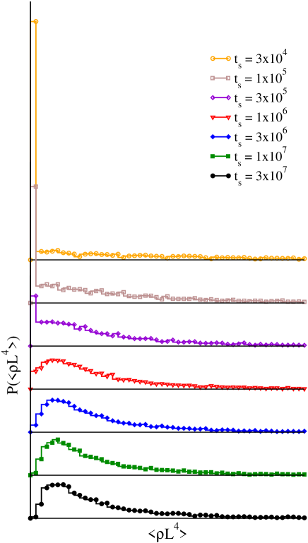
Figure 2: Evolution of the distribution of $\bm{\langle\rho L^{4}\rangle}$ as a function of $\bm{t_{s}}$ (the number of samples gathered at equilibrium for each disorder realization) for the same sample disorder realizations used in Fig. 1. The vertical axes are offset for clarity. The peak at $\bm{\langle\rho L^{4}\rangle=0}$ persists for $\bm{t_{s}\gg t_{r}}$, giving way to a broader peak at a non-zero $\bm{\langle\rho L^{4}\rangle}$. The distribution continues to change until $\bm{t_{s}\approx 3\times 10^{6}}$ upon which the distribution stops evolving.

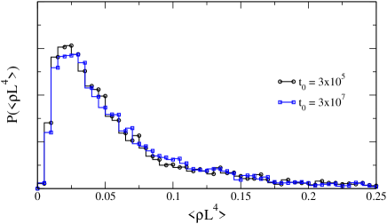
Figure 3: Distribution of $\bm{\langle\rho L^{4}\rangle}$ calculated with different ${\bf t_{0}}$ but the same $\bf{t_{s}}$ over two different sets of 1000 disorder realizations. The distribution is unchanged.

From these observations it would seem reasonable to generate $t_{s}=3\times 10^{5}$ configurations after equilibration at each disorder realization in order to calculate the disorder average. However, if we look more closely at the distribution $P(\langle\rho\rangle)$ generated by using $t_{s}=3\times 10^{5}$ configurations, we find a large peak in the distribution at $\langle\rho\rangle=0$ (see the uppermost graph of Fig. 2). For many disorder realizations, the Monte Carlo algorithm never generates an equilibrium configuration with a non-zero winding number (this can be verified by looking directly at the data set). If we generate more configurations at equilibrium for each disorder realization (that is, we increase $t_{s}$), the shape of the distribution changes—the peak at $\langle\rho\rangle=0$ shrinks and a broader one grows at a non-zero value. After one to three million sweeps, the peak at $\langle\rho\rangle=0$ disappears and the distribution stops evolving. This effect is a result of the discrete nature of the winding number, $n_{x}$, and the strong correlation between configurations generated by a successive Monte Carlo sweeps. Since the superfluid stiffness is defined in terms of $n_{x}$, it is difficult to numerically resolve the difference between a superfluid stiffness of zero and a small fractional value. For instance, a disorder realization with $\bar{\rho}L^{4}=0.05$ corresponds to an average squared winding number of $\langle\bar{n_{x}^{2}}\rangle=\frac{L_{\tau}}{L^{z}}\langle\rho L^{4}\rangle=1/160$, roughly implying that only one out of every 160 independent configurations has a non-zero winding number. Since the algorithm generates approximately one fully independent configuration every $t_{r}$ sweeps, at $t_{s}=3\times 10^{5}$ one would expect most runs to find $\langle\rho L^{4}\rangle=0$. (Here we assume that $t_{r}$ is proportional to the autocorrelation time $\tau$.) However, if the average is taken over a further $10^{2}$ independent configurations, the estimate will converge on the small but finite true average. Resolving the true shape of the distribution thus requires much longer runs at each realization of the disorder. That the lattice is in fact equilibrated at $t_{r}$ as determined by the convergence of the Hamming distances is supported by the fact one can generate the same distributions independent of $t_{0}$ (so long as $t_{0}>t_{r}$). Figure 3 shows the distribution of $\langle\rho L^{4}\rangle$ calculated over two different sets of 1000 disorder realizations, one with $t_{0}=3\times 10^{5}$, the other with $t_{0}=3\times 10^{7}$. In both cases $t_{s}=3\times 10^{7}$ configurations were generated after equilibration for each disorder realization.

An immediate conclusion to be drawn from these results is that, if attention is not paid to either the Hamming distances or the convergence of the complete distribution of the thermodynamic observables over the disorder, then one is very likely to be mislead by the results obtained. In particular, it is clear from the results in Figure 2 that if $t_{s}$ or $N_{D}$ are too small, then $[\langle\cdot\rangle]_{av}$ will be too small and the error bars will also be misleadingly small. As $t_{s}$ and $N_{D}$ are increased, $[\langle\cdot\rangle]_{av}$ will also likely increase due to the tails of the distribution while at the same time the associated error bars might very well remain roughly constant.

3 . Coupling Anisotropy

In the context of the Bose-glass to superfluid transition, one approach to improving the efficiency of the calculation is to increase the numerical value of the stiffness at the critical point. One possible means of achieving this is to increase the aspect ratio $\alpha$ between the spatial and temporal lattice sizes. In a finite system, the correlation length can be no longer than the size of the system; but since the temporal and spatial correlation length are related, a small $\alpha$ that truncates $\xi_{\tau}$ will in turn restrict $\xi$ to be smaller than the spatial extent of the lattice. Since a global current loop depends on correlation across the whole length of the lattice, this will limit the number of winding events and in turn reduce $\rho$. At the critical point, the value of $[\langle\rho L^{4}\rangle]_{av}$ should increase with $\alpha$ and it seems natural to assume that it will continue to increase at least up until $\xi_{\tau}/L_{\tau}\simeq(\xi/L)^{z}$, where $\alpha={\cal O}(1)$. Simulations are then best performed at this optimal aspect ratio; unfortunately they prove too large for us to simulate. The problem here is the relatively small probability of generating configurations with non-zero winding number in the spatial direction if a very small $\alpha$ is used. One could then ask if equivalent models can be found with higher winding numbers at $K_{c}$ for the same aspect ratio. Such models would likely have an optimal $\alpha$ at smaller values than the present one thereby decreasing the numerical overhead. It turns out that for the present model we can exploit the universality of the critical behavior to arrive at equivalent models that indeed have this desired property.

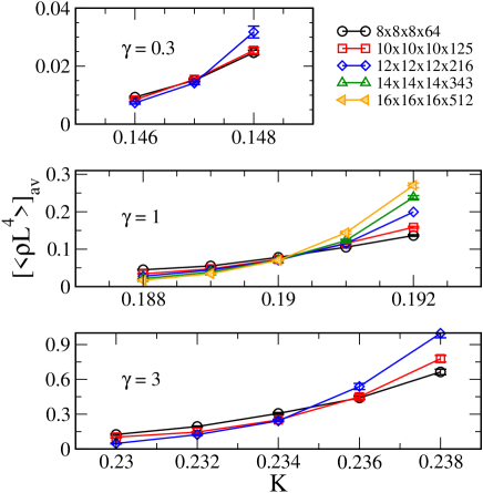
Figure 4: Crossings of $\bm{[\langle\rho L^{4}\rangle]_{av}}$ for three values of the anisotropy $\bm{\gamma}=$ 0.3, 1, and 3. The critical point increases as a function of $\bm{\gamma}$, as does the value of $\bm{[\langle\rho L^{4}\rangle]_{av}}$ at the critical point.

We now outline how we arrive at these equivalent models. The transformation from the Bose-Hubbard Hamiltonian to the effective link-current Hamiltonian described in Ref. [13] yields, near the end of the procedure, an anisotropic action

$$Z=\sum_{\bm{J}}\exp\bigg{\{}-\sum_{({\bf r},\tau)}\Big{[}\frac{K_{x}}{2}\bm{J^{\prime}}^{2}_{({\bf r},\tau)}$$

$$+\frac{K_{\tau}}{2}{J^{\tau}_{({\bf r},\tau)}}^{2}-\Delta\tau\bar{\mu_{{\bf r}}}J^{\tau}_{({\bf r},\tau)}\Big{]}\bigg{\}}$$ (14)

where $\Delta\tau$ is the width of each time slice, $\bm{J^{\prime}}=\sum_{\nu=x,y,z}J^{2}$, and

$$K_{t}=U\Delta\tau,\qquad K_{x}=-2\ln(-t\Delta\tau/2).$$ (15)

The simplest approach here is to set $KK_{x}=KK_{\tau}=1$, which yields the isotropic link-current model as stated above with $\mu_{{\bf r}}=\bar{\mu_{{\bf r}}}/U$. There is a freedom here, however: one can instead set $KK_{x}=1$ and $KK_{\tau}=\gamma$, and introduce an anisotropy between the space and time couplings in the link-current model without affecting the universal details:

$$H=\frac{1}{K}\sum_{({\bf r},\tau)}\bigg{\{}\frac{1}{2}\bm{J^{\prime}}^{2}_{({\bf r},\tau)}+\gamma\Big{[}\frac{1}{2}{J^{\tau}_{({\bf r},\tau)}}^{2}-\mu_{{\bf r}}J^{\tau}_{({\bf r},\tau)}\Big{]}\bigg{\}}.$$ (16)

The link-current couplings can be mapped back to the Bose-Hubbard tunneling and on-site disorder using (15):

$$\frac{U}{t}=2\gamma\big{(}Ke^{1/2K}\big{)}^{-1}.$$ (17)

If the transition occurs at a particular ratio $U/t$, an increase in $\gamma$ implies then an increase in $K_{c}$, for $K_{c}<1/2$. More importantly, increasing $\gamma$ freezes out the temporal dynamics of the link-current model. Both of these effects should speed up the spatial dynamics of the ‘worm’ algorithm, and since $\rho$ is defined in terms of these winding numbers, by changing $\gamma$ we can tune the value of $\rho L^{4}$ at the critical point. Figure 4 shows crossings in $\rho L^{4}$ for $\gamma=0.3$, 1, and 3. As expected, increasing $\gamma$ increases the value of $K_{c}$ and the magnitude of the stiffness at the crossing, hence improving the sampling efficiency of the algorithm. Note that this has been achieved without changing the aspect ratio, $\alpha$.

Due to space constraints we do not show results for the critical exponents at different $\gamma$. However, we have studied them in detail and they are indeed independent of $\gamma$ as one would expect from universality arguments. We note that it would be of considerable interest to study the evolution of the distribution of thermodynamic variable, as shown in Fig. 2 for $\gamma=1$, for different values of $\gamma$. Preliminary results indicates that the width of the distributions vary with $\gamma$, likely increasing monotonically with this parameter. Due to time constraints we leave a detailed investigation for future study.

4 . Conclusions

Numerical studies of disordered systems are notoriously difficult due to the large amount of computational resources required and to the many subtle sources of systematic error. The procedure we have presented to estimate disorder distributions and their averages highlights some of the potential pitfalls. Under-sampling the disorder distribution (setting $N_{D}$ too low), under-sampling each individual distribution (setting $t_{s}$ too low), and failing to properly equilibrate each simulation (setting $t_{0}$ too low) can all lead to erroneous estimates. The two procedures presented above provide confirmation that these pitfalls have been avoided. The convergence of the Hamming distances provides a measure of $t_{r}$ and confirms that the Monte Carlo simulations are generating equilibrium configurations. The disorder distributions themselves can contain artifacts of the Monte Carlo averaging procedure; they should not demonstrate any dependence on $t_{0}$ or $t_{s}$ if these have been set sufficiently large. These procedures can be generalized to other systems.

In the context of the Bose-Hubbard model, the discrete nature of the winding number in the link-current representation forces the investment of a large amount of computational resources in simulating each individual disorder realization ($t_{s}$ must be set much greater than $t_{r}$). However, by adjusting the anisotropy between the spatial and temporal coupling strengths in the link-current model, we can increase the magnitude of the superfluid stiffness at the critical point. This improves the numerical efficiency of the calculation without affecting the universal details of the critical behaviour. This observation may prove useful for future Monte Carlo studies of the Bose-Hubbard model in the link-current representation.

References

- [1] A. Aharony and A. B. Harris. Absence of self-averaging and universal fluctuations in random systems near critical points. Phys. Rev. Lett., 77:3700, 1996.
- [2] A. Aharony, A. B. Harris, and S. Wiseman. Critical disordered systems with constraints and the inequality . Phys. Rev. Lett., 81:252, 1998.
- [3] K. Bernadet, F. Pázmándi, and G. G. Batrouni. Disorder averaging and finite size scaling. Phys. Rev. Lett., 84:4477, 2000.
- [4] R. N. Bhatt and A. P. Young. Numerical studies of ising spin glasses in two, three, and four dimensions. Phys. Rev. B, 37:5606, 1988.
- [5] J. T. Chayes, L. Chayes, D. S. Fisher, and T. Spencer. Finite-size scaling and correlation lengths for disordered systems. Phys. Rev. Lett., 57:2999, 1986.
- [6] M. P. A. Fisher, P. B. Weichman, G. Grinstein, and D. S. Fisher. Boson localization and the superfluid insulator transition. Phys. Rev. B., 40:546, 1989.
- [7] M. Greiner, O. Mandel, T. Esslinger, T. W. Hänsch, and I. Bloch. Quantum phase transition from a superfluid to a mott insulator in a gas of ultracold atoms. Nature, 415:39, 2002.
- [8] I. F. Herbut. Critical behavior at superconductor-insulator phase transitions near one dimension. Phys. Rev. B, 58:971, 1998.
- [9] I. F. Herbut. Quantum critical points with the coulomb interaction and the dynamical exponent: When and why z = 1. Phys. Rev. Lett., 87:137004, 2001.
- [10] P. Hitchcock and E. Sørensen. Bose-glass to superfluid transition in the three-dimensional boson hubbard model. preprint, cond-mat/0601182, 2006.
- [11] F. Pázmándi, R. T. Scalletar, and G. T. Zimányi. Revisiting the theory of finite size scaling in disordered systems: can be less than 2/d. Phys. Rev. Lett., 79:5130, 1997.
- [12] R. Sknepnek and T. Vojta. Smeared phase transition in a three-dimensional ising model with planar defects: Monte carlo simulations. Phys. Rev. B, 69:174410, 2004.
- [13] M. Wallin, E. Sørensen, S. Girvin, and A. P. Young. Superconductor-insulator transition in two-dimensional dirty boson systems. Phys. Rev. B, 49:12115, 1994.