Phase equilibrium in two orbital model under magnetic field

Abstract

The phase equilibrium in manganites under magnetic field is studied using a two orbital model, based on the equivalent chemical potential principle for the competitive phases. We focus on the magnetic field induced melting process of CE phase in half-doped manganites. It is predicted that the homogenous CE phase begins to decompose into coexisting ferromagnetic phase and CE phase once the magnetic field exceeds the threshold field. In a more quantitative way, the volume fractions of the two competitive phases in the phase separation regime are evaluated.

Manganites, a typical class of strong correlated electron systems, have been intensively studied in the last decade, due to their unusual behaviors of potential applications such as colossal magnetoresistance (CMR). The double exchange (DE) mechanism can explain the magnetic transition qualitatively, but more complex mechanism responsible for CMR is not yet fully understood. The idea of phase separation (PS) was recently proposed to understand the physics essence underlying the amazing behaviors of manganites, while more and more theoretical and experimental evidences confirm the existence of PS due to the intrinsic inhomogeneity Dago ; review ; Uehara .

Former investigations on the phase diagram of manganites revealed the first-order character of phase transitions between various phases, e.g. charge-ordered (CO) insulator and ferromagnetic (FM) metal review ; Loudon ; Mura ; Aliaga . The insulator-metal transition in manganites can be reasonably understood as the consequence of percolation of FM metal filaments embedded in the insulated matrix, and there are plenty of experimental evidences to support this PS framework review ; Zhang ; Tokunaga . Current theories on manganites mainly stem from the competition between several interactions: DE, super exchange, Hund coupling, electron-phonon interaction and Coulomb interaction review . Besides, the effect of quench disorder on PS dynamics is highlighted, especially on the large scale PS. The theoretical progress has enabled us to sketch the phase diagram in some special regimes from calculation and identify the PS regime in parameter space with various microscopic models Yunoki1 ; Yunoki2 ; Yunoki3 . Nevertheless, it is still unclear theoretically how the PS develops, especially under an external perturbation, e.g. magnetic or electric field. In other word, it is of interest to not only identify the existence of PS regime, but also concern how the phase separation occurs and how it evolves upon external perturbation, because potential applications call for more sufficient theoretical interpretation. For instance, the CMR effect, which is one of the most attracting topics in the physics of manganites, may be described by the resistor network model phenomenologically, based on the percolation mechanism. In such case the volume fraction of metal phase is the key input variable, which, however, lacks credible theoretical investigation yet. In earlier studies, this important variable was obtained from experiment or toy model Mayr ; Dong .

In this letter, we attempt to study the phase equilibrium (PE) in a two orbital model. We emphasize particularly the evolvement of PS upon the magnetic field perturbation. So we call it PE instead of PS in this work. Let’s begin with a simplified model Hamiltonian which has been frequently used review :

$$Hami. = -\sum\limits_{\boldsymbol{i\alpha}\gamma\gamma^{\prime}\sigma}t_{\gamma\gamma^{\prime}}^{\boldsymbol{\alpha}}d_{\boldsymbol{i}\gamma\sigma}^{{\dagger}}d_{\boldsymbol{i}\gamma^{\prime}\sigma}-J_{H}\sum_{\boldsymbol{i}}\boldsymbol{s}_{{}_{\boldsymbol{i}}}\cdot\boldsymbol{S}_{i}$$ (1)

$$+J_{AF}\sum_{<\boldsymbol{i},\boldsymbol{j}>}\boldsymbol{S}_{i}\cdot\boldsymbol{S}_{j}+\boldsymbol{H\cdot}\sum_{\boldsymbol{i}}g\boldsymbol{(s}_{i}+\boldsymbol{S}_{i})$$

where $\boldsymbol{\alpha}$ is the vector connecting nearest-neighbor (NN) sites and $d_{\boldsymbol{i}\gamma\sigma}^{{\dagger}}$($d_{\boldsymbol{i}+\boldsymbol{\alpha}\gamma^{\prime}\sigma}$) is the generation (annihilation) operator for $e_{g}$ electron with spin $\sigma$ in the $\gamma$($\gamma^{\prime}$)-orbital on site $\boldsymbol{i}$($\boldsymbol{i}+\boldsymbol{\alpha}$); $t_{rr^{\prime}}^{\boldsymbol{\alpha}}$ is the NN hopping amplitude between $\gamma$ and $\gamma^{\prime}$-orbital ($d_{x^{2}-y^{2}}$ as $a$ orbital, $d_{3z^{2}-r^{2}}$ as $b$ orbital) along $\boldsymbol{\alpha}$-direction, with $t_{bb}^{z}=t_{0}>0$ ($t_{0}$ is taken as energy unit), $t_{aa}^{x}=t_{aa}^{y}=\frac{3}{4}t_{0}$, $t_{bb}^{x}=t_{bb}^{y}=\frac{1}{4}t_{0}$, $t_{ab}^{y}=t_{ba}^{y}=-t_{ab}^{x}=-t_{ba}^{x}=\frac{\sqrt{3}}{4}t_{0}$, $t_{aa}^{z}=t_{ab}^{z}=t_{ba}^{z}=0$, respectively; $\boldsymbol{S}_{i}$ is the spin operators for $t_{2g}$ core on site $\boldsymbol{i}$, while $\boldsymbol{s}_{i}$ for $e_{g}$ itinerant electron. The first term represents the kinetic energy (DE process) which leads to FM spin arrangement. The second term is the Hund coupling of $e_{g}$ and $t_{2g}$ electrons where $J_{H}>0$ is large enough to be regarded as infinite, so the spin of $e_{g}$ electron is always parallel with the same-site $t_{2g}$ spin. The super exchange interaction $J_{AF}>0$ prefers to couple NN $t_{2g}$ spins antiferromagnetically; The last term represents the magnetic field contribution with magnetic field $H$ and Lande factor $g$. The electron-phonon coupling and Coulomb repulsion are not taken into account in this Hamiltonian and their effect on PE will be discussed below.

The above simplified Hamiltonian can be solved exactly once a prior $t_{2g}$ spin pattern is given. In real manganites, various $t_{2g}$ spin patterns exist corresponding to abundant phases, e.g. FM, antiferromagnetic (AFM), CO, orbital-ordered (OO) phases. In this work, several typical $t_{2g}$ patterns confirmed from experiments: C-type AFM (CAFM), G-type AFM (GAFM), FM and CE phase are chosen as the candidates to compare. The CAFM phase is constructed by antiferromagnetically coupled one-dimension FM lines, while the CE phase is constructed by antiferromagnetically coupled one-dimension zigzag FM chains and is found to be CO/OO Wollan ; Good ; Brink . The GAFM takes the familiar AFM arrangement in all three directions. Then the Hamiltonian can be exactly solved when the Hund factor $J_{H}$ is simplified as infinite. The procedure of derivation is straightforward and the details can be found in Ref.review . Then density of state (DOS, $D(E)$) of the these phases can be calculated from the dispersion relationship using numerical method, as shown in Fig.1(a). In addition, the chemical potential $\mu$ of these phases is obtained simultaneously by integrating the DOS, as shown in Fig.1(b). Consequently, the ground state energy is calculated. For instance, the energy of FM phase can be written as:

$$\frac{E(n,H)}{N}=\frac{1}{N}\int^{E<\mu}D(E)EdE+\frac{27}{2}J_{AF}-3H$$ (2)

here $N$ is the number of whole sites and is infinite ideally. The first integral term gives the energy of all $e_{g}$ electrons; term $27J_{AF}/2$ arises from the six NN FM correlation between $|\boldsymbol{S}|=3/2$ $t_{2g}$ cores in classical approximation; factor $3$ before $H$ is calculated by multiplying $t_{2g}$ spin $3/2$ with Lande factor $2$. Besides, the influence of $H$ on $D(E)$ has also been taken into account. The average $e_{g}$ electron concentration $n\in[0,1]$. The DOS, chemical potential and ground energy of other phases can also be calculated exactly just as the FM case.

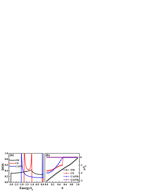
Figure 1: (color online) (a)Density of state of FM/CE/CAFM phase. Here only regime $E\leq 0$ is displayed since the symmetrical $E>0$ part is empty in ground state. In GAFM, there is only a single energy level at $0$ because of the localization of $e_{g}$ electron. (b)Chemical potential $\mu$ as a function of $e_{g}$ electron concentration. The energy gap $t_{0}$ for the CE phase at $n=0.5$ is evident both in (a) and (b).

However, what should be noted is that none of these phases can be stable over the whole doping range. In order to determine which phase is the preferred one at a given concentration, the ground state energy of these phases, when $J_{AF}$ is set as $0.0278t_{0}$ and $H=0$, is plotted in Fig.2. The preferred ground state is the energy minimal state. It should be GAFM as $n\thicksim 0$ because the interaction is almost pure AFM super exchange. As $n\thicksim 0.3$, the preferred state is CAFM. The CE phase can appear only in a narrow regime $n\thicksim 0.5$. When the gain from kinetic energy suppresses the loss of super exchange energy in the large $n$ regime, the FM becomes the stable phase. With this calculation, the phase diagram over the whole concentration regime has be developed. Of course, the phase diagram of real manganites is more complex than this simple sketch for two reasons: first, the Hamiltonian Eq.(1) is oversimplified and secondly the candidate phases chosen here are not complete but only four phases. Even though, the calculated phase diagram is quite similar to that of some typical manganites (zero-temperature): e.g. Nd_1-xSr_xMnO₃ (here $n=1-x$) Kaji . In fact, it is shown that the phase diagram of other manganites: e.g. La_1-xSr_xMnO₃ or Pr_1-xCa_xMnO₃, can be reproduced roughly by adjusting the value of $J_{AF}$, whose role will be revisited below. An important truth revealed here is that no matter what $J_{AF}$, the CE phase can either appear in the narrow regime $n\thicksim 0.5$ or simply be unstable over the whole concentration regime.

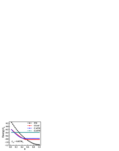
Figure 2: (color online) System energy $E$ (ground state under zero field) as a function of $e_{g}$ electron concentration $n$, with $J_{AF}=0.0278t_{0}$. Upon increasing $e_{g}$ electrons $n$, a transition sequence of the ground state: GAFM$\rightarrow$CAFM$\rightarrow$CE$\rightarrow$FM, is shown. The CE phase as ground state is possible only in the narrow range around the half-filling point.

The above theoretical approach based on Hamiltonian Eq.(1), whose origin can be found from Ref.review , allows us to study the PE in PS regime. Here, a simple but representative case: the PE between FM phase and CE phase with $n=0.5$, will be studied. It corresponds to the melting process of a type of CO state (here it is CE phase) under external magnetic field. Since for FM metallic phase the lattice distortions are absent and the $e_{g}$ electrons are delocalized Ahn , the electron-phonon coupling and on-site Coulomb repulsion are unimportant. On the other hand, the CE phase can also be reasonably described as a band insulator by this Hamiltonian at $n=0.5$ case review ; Brink . Therefore, Eq.(1) is suitable to deal with the PE between FM metallic phase and CE phase, noting that Eq.(1) can be exactly solved without scale issue.

The PE principle for a PS system can be represented by the equivalence in chemical potential between the competitive phases, i.e. FM and CE to be considered. From the above calculation (Fig.1(b)), it is seen that at $n=0.5$ and under zero field, the chemical potential of pure FM phase is about $-1.52t_{0}$ and that of CE phase is $-t_{0}$. Therefore, the chemical potential $\mu$ for the possible PS system would be in the range [$-1.52t_{0}$, $-t_{0}$]. The sum of $e_{g}$ electrons in the FM and CE phases can be calculated:

$$n_{A}=\frac{p_{A}}{N}\int^{E<\mu}D(E)dE$$ (3)

here $p_{A}$ is the volume fraction of $A$ (FM/CE) phase. The upper limit of the integral should meet the equivalent chemical potential condition: $\mu_{FM}=\mu_{CE}=\mu$. Then the following set of equations yields:

$$\left\{\begin{array}[]{c}p_{FM}+p_{CE}=1\\ n_{FM}+n_{CE}=0.5\end{array}\right.$$ (4)

By numerical method, Eq.(4) can be solved with the prior assumed $\mu$. Given parameters $J_{AF}=0.0278t_{0}$ and $H=0$, the calculated relative volume fraction of FM/CE phase as a function $\mu$ are shown in Fig.3(a) (right axis). Then by including the factor $p_{A}$ into the energy equation, the total system energy: $E=p_{FM}E_{FM}+p_{CE}E_{CE}$ can been calculated, as shown in Fig.3(a) (left axis). It is seen that both $p_{FM}$ and $E$ are monotonously decreasing functions of $\mu$. The ground state must be homogenous CE phase because the PS state goes against energy. In case of nonzero magnetic field (e.g. $H=0.015t_{0}$), the above calculation is repeated by taking the magnetic field contribution to DOS and energy into account. The results are plotted in Fig.3(b). Quite interestingly, a nonzero field results in a minimal in the $E-\mu$ curve (here at $\mu\thicksim-1.13t_{0}$). The PS state associated with this minimal energy point is more stable with respect to the homogenous FM or CE phase. The value $-1.13t_{0}$ is the real chemical potential of this PS ground state which consists of $57\%$ CE phase and $43\%$ FM phase.

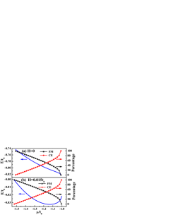
Figure 3: (color online) Volume fraction of FM/CE phase (right axis) and corresponding total energy system $E$ (left axis) as a function of chemical potential $\mu$. $J_{AF}=0.0278t_{0}$. (a)Zero field case. where the ground state is CE phase without phase separation because the energy decreases monotonously with chemical potential; (b)under magnetic field $H=0.015t_{0}$, where a energy minimal appears at $\mu=-1.13t_{0}$. The coexistence with the fraction of FM and CE phase in this point is the ground state.

By varying the value of $H$, one can repeat the above calculation and then obtain the relative volume fractions of the two phases as a function of $H$, as shown in Fig.4(a). When $H$ is low (below the lower threshold $H_{min}\thicksim 0.0069t_{0}$), the CE phase is robust against magnetic field perturbation, indicating the stable and homogenous CE phase as the ground state. Upon an increasing of $H$ beyond $H_{min}$, part of the CE phase begins to melt into FM phase, and $p_{CE}$ is deceasing with increasing $H$ under the equivalent chemical potential condition. In details, $p_{FM}$ increases rapidly once $H>H_{min}$, and the growth becomes slower when $H$ is further higher, as shown in Fig.4(a). Note here that the threshold of percolation for FM phase can be easily surpassed under a field slightly higher than $H_{min}$. For instance, only a field of $H=0.009t_{0}$ is needed to obtain a FM phase of $24.7\%$ (threshold for a three-dimensional simple cubic bond percolation), beyond which an insulator-metal transition may be expected. When $H$ is extremely high (not shown in Fig.4(a)), the equivalent chemical potential condition can no longer be satisfied, indicating a termination of the PS state and the ground state will be homogenous FM state.

The above calculation indicates that the lower threshold of magnetic field to melt the CE phase is $0.0069t_{0}$. Considering that $t_{0}$ in low-bandwidth manganites is small, e.g. $0.1eV$, the calculated $H_{min}$ is about $12T$, a value consistent with the experimental data Kuwa ; Tomi ; Toku ; Okim . Note here that $H_{min}$ is not equal the direct energy gap between FM and CE phase, which is one order of magnitude larger than experimental value (shown in Fig.2, about $0.08t_{0}$). It means that the required magnetic field to destroy the CO insulator is strongly reduced by PS which can occur once the energy of competitive phases is close to each other. On the other hand, as identified earlier, parameter $J_{AF}$ plays a key role in PS although it is the least intrinsic interaction in manganites review . Other than the above case of field-induced sequences, abundant phenomena associated with PS in manganites can be predicted by our model through adjusting $J_{AF}$. For example, again at $n=0.5$, a coexistence of FM phase and CE phase under zero field is predicted at $0.019t_{0}<J_{AF}<$ $0.026t_{0}$. When $J_{AF}$ is further reduced, a homogeneous FM phase as the ground state is possible even under zero field. The transition between three regimes: homogenous FM phase to PS state to homogenous CE phase, are identified in Fig.4(b). These transitions can be mapped to real manganites of wide-band to those of middle-band and then narrow-band review .

Figure 4: (a)Melting process of the CE phase under magnetic field. When the field is below the threshold $H_{min}$, the homogenous CE phase is robust. Then phase separation occurs when $H>H_{min}$. (b) Phase transitions induced by $J_{AF}$ under zero-field condition: FM phase at weak $J_{AF}$; coexistence of FM and CE phase at middle $J_{AF}$; CE phase at strong $J_{AF}$.

It should be mentioned that the only parameter adjustable here is the super exchange $J_{AF}$, and the energy difference between different phases is dependent on ratio $J_{AF}/t_{0}$. This is obviously oversimplified, referring to real manganites materials in which not only the double/super exchange but also the Jahn-Teller distortion and Coulomb repulsion play important roles. For instance, the Jahn-Teller distortion in CE phase will affect the energy band and DOS Brey ; Dong2 . In addition, although the phase diagram given in Fig.2 is quite similar to those for some manganites, there are still some blemishes. For instance, a prediction of the correct concentration $n$ corresponding to the A-type AFM observed in LaMnO₃ ($n\thicksim 1$) Wollan or Nd_1-xSr_xMnO₃ ($x\thicksim 0.55$) Kaji can not be given by the present model. However, if a complete Hamiltonian is employed, the calculation has to be oversimplified, e.g. limited in a small cluster which is disadvantageous to deal with PS. Fortunately, Eq.(1) in the present work can describe FM/CE phase to some satisfactory extent and it is a good starting point to investigate the PE issue in PS systems against external magnetic field perturbation. Furthermore, the present approach represents a general roadmap to investigate the PE issues in manganites: e.g. phase competition other than FM-CE, of more than two phases, of different $e_{g}$ concentrations, and effect of other perturbation than magnetic field etc. The key condition is the equivalence of chemical potential between competitive phases.

In summary, the principle of chemical potential equivalence has been introduced to investigate the phase equilibrium of half-doped manganites under external magnetic field. By employing the two orbital model, we have presented an explicit solution to the phase equilibrium between FM phase and CE phase. The magnetic field threshold required for melting of the CE phase has been calculated, consistent with the experimental results. The volume fractions of the two competitive phases in the phase separation regime as a function of external magnetic field have been evaluated. In addition, the super exchange modulated transitions between ferromagnetic, phase separated and CE states under zero-field, is predicted.

- (1) E. Dagotto, Science 309, 257 (2005).
- (2) E. Dagotto, Nanoscale Phase Separation and Colossal Magnetoresistance (Springer-Verlag, Berlin, 2002).
- (3) M. Uehara, S. Mori, C. H. Chen, and S.-W. Cheong, Nature 399, 560 (1999).
- (4) J. C. Loudon, N. D. Mathur, and P. A. Midgley, Nature 420, 797 (2002).
- (5) S. Murakami and N. Nagaosa, Phys. Rev. Lett. 90, 197201 (2003).
- (6) H. Aliaga et al., Phys. Rev. B 68, 104405 (2003).
- (7) L. Zhang et al., Science, 298, 805 (2002).
- (8) M. Tokunaga, H. Song, Y. Tokunaga, and T. Tamegai, Phys. Rev. Lett. 94, 157203 (2005).
- (9) S. Yunoki et al., Phys. Rev. Lett. 80, 845 (1998).
- (10) S. Yunoki, A. Moreo, and E. Dagotto, Phys. Rev. Lett. 81, 5612 (1998).
- (11) S. Yunoki, T. Hotta, and E. Dagotto, Phys. Rev. Lett. 84, 3714 (2000).
- (12) M. Mayr et al., Phys. Rev. Lett. 86, 135 (2001).
- (13) S. Dong, H. Zhu, X. Wu, and J.-M. Liu, Appl. Phys. Lett. 86, 022501 (2005).
- (14) E. O. Wollan and W. C. Koehler, Phys. Rev. 100, 545 (1955).
- (15) J. B. Goodenough, Phys. Rev. 100, 564 (1955).
- (16) J. van den Brink, G. Khaliullin, and D. Khomskii, Phys. Rev. Lett. 83, 5118 (1999).
- (17) R. Kajimoto et al., Phys. Rev. B 60, 9506 (1999).
- (18) K. H. Ahn, T. Lookman, and A. R. Bishop, Nature 428, 401 (2004).
- (19) H. Kuwahara et al., Science 270, 961 (1995).
- (20) Y. Tomioka et al., Phys. Rev. B 53, 1689(R) (1996).
- (21) M. Tokunaga, N. Miura, Y. Tomioka, and Y. Tokura, Phys. Rev. B 57, 5259 (1998).
- (22) Y. Okimoto et al., Phys. Rev. B 59,7401 (1999).
- (23) L. Brey, Phys. Rev. B 71, 174426 (2005).
- (24) S. Dong et al., cond-mat/0508673.