Spinless Fermionic ladders in a magnetic field: Phase Diagram

Abstract

The system of interacting spinless fermions hopping on a two-leg ladder exhibits a series of quantum phase transitions when subjected to an external magnetic field. At half filling, these are either $U(1)$ Gaussian phase transitions between two phases with distinct types of long-range order or Berezinskii-Kosterlitz-Thouless transitions between ordered and gapless phases.

I Introduction

The behavior of interacting electron systems under the action of an external magnetic field, affecting orbital motion of the particles, is a subject of intense research of the last several decades. It has long been established that the magnetic field has a dramatic effect on all properties of the system. Even in the absence of interaction, the spectrum of the free Fermi gas is modified and exhibits Landau quantizationlan in the continuum or the Hofstadter spectrumhof on a two-dimensional (2D) lattice. The most spectacular consequence of this phenomenon is the Quantum Hall Effect (QHE).qhe Electron-electron interaction compounds the complexity of the problem, giving rise to the Fractional Quantum Hall Effect (FQHE).fhe

The current theoretical understanding of the effect of the magnetic field on the properties of electron systems was achieved by a combination of various methods and techniques, each of which is strictly speaking only applicable in a certain parameter range. What is still lacking is a comrehensive approach that would unify all of the different aspects of the problem into a single coherent picture. Perhaps at present such a goal is too ambitious. However, as a first small step in this direction, one can ask whether such a comprehensive approach can be formulated for a simpler model, that would on one hand be a problem of interacting electrons in the magnetic field and on the other hand would, at least in principle, allow a generalization towards the original problem.

The simplest model of interacting fermions that incorporates orbital effects of an external magnetic field is that of spinless fermions hopping on a two-leg ladder. This model is simple enough not to exhibit the multitude of small gaps in the single-particle spectrum (characteristic of the Hofstadter problemhof ). Yet the magnetic flux piercing the plaquettes of the ladder changes the ground state properties of the system giving rise to non-trivial phases and inducing quantum phase transitions.

Ladder modelsthl ; fab occupy a special place in the field of strongly correlated electron systems. On one hand, they describe (at least within some range of temperatures) behavior of many naturally found compoundsex1 , including carbon nanotubes,ex2 ; th4 as well as artificially manufactured structures.ex3 On the other hand, they provide a fertile ground for application of theoretical techniques developed for one-dimensional systemsth1 - i.e. non-perturbative approaches leading to asymptotically exact results. Furthermore, they are a first step for various attempts at generalization of the lore of physics in one spatial dimension to higher-dimensional problems.th2

As is often the case, situations where the number of particles is commensurate with the lattice attract the most attention since only then can long range order (LRO) develop. We have previously shownus that at a quarter filling, the presence of the flux results in exciting effects which do not exist in the absence of the flux. In particular the uniform external magnetic field can lead to a staggered flux (or orbital antiferromagnet) phase, which furthermore has fractionally charged excitations.

The purpose of the present paper is to describe the full phase diagram of interacting spinless fermions on the two-leg ladder at $1/2$-filling in the presence of an external magnetic field. To drive a system to criticality by applying the magnetic field is an intriguing possibility which should be more accessible in experiment than varying coupling constants. The phase diagram displays a multitude of quantum phase transitions induced by the flux. There are two types of these phase transitions: (i) Berezinskii-Kosterlitz-Thouless (BKT) transitionsbkt between ordered and disordered ground states, and (ii) $U(1)$ Gaussian phase transitions between different ordered ground states. Here we choose the fermions to be spinless in order to eliminate Zeeman splitting and focus on the orbital effects of the magnetic field. The case of spin-1/2 particles will be discussed in a separate publication.

Traditionally gia ; boz ladder models have been treated in two complimentary approaches. On one hand, one can start with the model of two decoupled chains, define the low energy effective theory for each of them, and then treat both the single-particle transverse hopping and two-particle inter-chain correlations perturbatively.nlk93 On the other hand, one could start with the exact single particle basis (given by two bands) and then proceed with the corresponding low energy limit.fab For the major part of this paper we will be using the latter approach which allows us to treat intra- and inter-chain processes on equal footing. However, it is well known and (at least in the absence of the magnetic field) that for weak enough inter-chain tunneling there exists the phenomenon of Anderson confinement, i.e. the suppression of the inter-chain single-particle tunneling by intra-chain two-particle correlations. This effect can be seen in either picture, but it is more intuitive to discuss it within the chain approach. Both ways should produce the same physical results, but understanding the relation between the two approaches allows us to establish the limits of applicability of the effective low energy theories that can be derived within either picture. Moreover, we discuss how the Anderson confinement regime is affected by the magnetic flux.

The remainder of the paper is organized as follows. We start by defining the microscopic Hamiltonian of the model and proceed directly to the results, discussing the phase diagram and the other physical properties of the model. Then we outline the details of the calculations within the weak coupling (bosonization) approach. In Section III we derive the effective low energy theory in the band picture. In Section IV we turn to the chain picture and discuss its relation to the band approach. Section V is devoted to the strong coupling limit of our model and is followed by a brief summary of the results. Mathematical details are relegated to Appendices.

II Model and results

In this section we present our results. We start by defining the microscopic Hamiltonian of our model and proceed to discuss the zero-temperature phase diagram.

II.1 The Hamiltonian

We consider a tight-binding model of spinless fermions on a two-leg ladder described by the Hamiltonian

$$H= - \frac{1}{2}\sum_{i\sigma}\left[t_{\parallel}(\sigma)c_{i,\sigma}^{\dagger}c_{i+1,\sigma}+h.c.\right]-t_{\perp}\sum_{i\sigma}c_{i,\sigma}^{\dagger}c_{i,-\sigma}$$ (1)

$$+ U\sum_{i}n_{i+}n_{i-}+V\sum_{i\sigma}n_{i,\sigma}n_{i+1,\sigma}.$$

Here $c_{i,\sigma}$ is the electron annihilation operator on the chain $\sigma=\pm$ at the site $i$; $n_{i\sigma}=c^{\dagger}_{i,\sigma}c_{i,\sigma}$ are the occupation number operators; $t_{\perp}$ and $t_{\parallel}$ are the transverse and longitudinal hopping amplitudes, respectively. The last two terms in Eq. (1) describe nearest neighbour inter- and intra-chain interactions. The chosen form of short-range interaction is quite representative because it reflects the generic symmetry of the ladder and yields the most general effective field theory in the low-energy limit. Our notation reflects the well-known analogy between ladder models of spinless fermions and Hubbard-like chains of spin-1/2 particles. In our case however, the $SU(2)$ symmetry is explicitly broken in the Hamiltonian (1) by the inter-chain hopping and the $V$ interaction term (the former is analogous to a Zeeman energy due to an external magnetic field alng the $x$-axis, while the latter is a counterpart of an exchange anisotropy along the $z$-axis).

The external magnetic field $B$ is introduced by means of the Peierls substitution.pei In the Landau gauge dau with the vector potential ${\bf A}=B(-y,0,0)$ the transverse hopping term is independent of the field, while the longitudinal hopping amplitude can be written as

$$t_{\parallel}(\sigma)=t_{0}e^{i\pi\sigma f},$$ (2)

where $f$ is the magnetic flux through the elementary plaquette in units of flux quantum $\phi_{0}=hc/e$. Expressed in terms of the flux the model is explicitly gauge invariant.

Figure 1: Cartoon depictions of possible ordered phases at $1/2$ filling. The dots represent excess fermion dimerization on the sites. The ellipses represent excess occupation on the bonds. The arrows represent local currents. Note that the OAF and the BDW coexist - see Section III for an explanation.

II.2 Phase Diagram

At half filling (one fermion per rung) the model (1) is characterized by a rather rich phase diagram. Depending on the values of microscopic parameters the ground state of the model may posess true long range order. Possible ordered phases are illustrated in Fig. 1. The cartoons show a strong-coupling picture of the phases: charge density waves (CDW), where particles are localized on sites of the ladder; bond density waves (BDW) with dimerized links along the chains; and the orbital antiferromagnetnlk93 (OAF), sometimes referred to as the staggered flux phase or a d-density wave, where the particle density remains uniform, but there exist non-vanishing local currents that have opposite directions on alternate bonds. Notice that, in the spin language, the Relative CDW is similar to a spin density wave (SDW) with spins polarized along $z$ (a Neel state SDW^z), whereas the OAF is equivalent to a SDW^y.

In addition, the model (1) allows for various phases that do not posess long-range order. Using the aforementioned analogy with the Hubbard chain, we may discuss the model (1) in terms of “spin” (or “relative”) and “charge” (or “total”) sectors. In Section III.2 we show that, in the low-energy limit, the “charge” and “relative” sectors of the model asymptotically decouple. In all of the ordered phases both sectors are gapped. However, it is possible to have a phase where only one of the sectors acquires a spectral gap. Phases where only the “charge” sector is gapped, irrespective of the type of dominant correlations, we will call the Mott Insulator (MI). The cases where the gap exists in the “relative” sector only will be called the Luther-Emery Liquid (LEL).lel Finally, when both sectors are gapless, the system represents a Luttinger Liquid (LL).

Figure 2: Phase diagram at $B=0$ (after Ref. boz, ). Phase boundaries correspond to the lines $V=0$, $U/2V=-2+\tau^{2}$ and $U/2V=-\tau^{2}$.

The phase diagram in the absense of the flux is known.gia ; boz For the sake of clarity we include it in Fig. 2. This phase diagram is valid for suffiently large values of $t_{\perp}$ where delocalization of the fermions across the rungs suppresses the CDW phase (which happens in the absence of the inter-chain tunneling). There are two ordered phases: (i) for purely repulsive interactions $U,V>0$, one has a relative CDW as to be expected (see Section V); (ii) for repulsive interchain interaction and not too strong attractive in-chain interaction, the ground state is the orbital antiferromagnet.ner ; nlk93 The phase diagram in Fig. 2 was obtained within a weak-coupling bosonization approach. The phases do exist when the coupling becomes strong, however the exact location of the phase boundaries might change.

Once the magnetic field is applied, the system may exhibit additional phase transitions. In Fig. 3 we plot the entire weak-coupling phase diagram for the model at half-filling and sufficiently large $t_{\perp}$ (see next subsection). The magnetic flux varies along the vertical axis, so that the diagram in Fig. 2 corresponds to the bottom axis of Fig. 3. The ratio of the microscopic interaction parameters of the Hamiltonian (1), $U/2V$, is represented in Fig. 3 through the angular variable $\theta=\tan^{-1}U/2V$ which varies along the horizontal axis. Four different regions corresponding to various signs of the constants $U$ and $V$ are indicated on the upper horizontal line in Fig. 3. The analytic description of the phase boundaries, based on the weak coupling theory, is given in Appendix A. The position of the boundaries depends on the applied field, the ratio $U/2V$ (i.e. $\theta$) and the ratio of the hopping parameters, $\tau=t_{\perp}/t_{0}$. We plot the phase diagram as a function of $\theta$ and flux for $\tau=0.25$, the value is arbitrary but representative as long as $\tau$ exceeds a possible gap in the “relative” sector. At other values of $\tau$ the topology of the phase diagram and classification of the phases do not change qualitatively. Similarly, if we modify our model (1) to include other short-range interaction terms, the only effect on the phase diagram would again be just the shift of the phase boundaries.

Let us now describe the phase transitions induced by the applied field (i.e. the vertical direction in Fig. 3). We assume that the inter-chain hopping parameter $\tau$ is not too small (see next subsection). Note, that since the model (1) is invariant under the transformation $f\rightarrow 1-f$, $\sigma\rightarrow-\sigma$,we only need to consider the flux within the range $0<f<1/2$. Moreover, when the flux is large enough, $\sin^{2}\pi f>1-\tau^{2}$, there is a band gap in the single particle spectrum of the model. That state is largely unaffected by interaction effects (at least within the weak-coupling limit), and thus we will restrict our discussion to smaller values of $f$. While the weak-coupling approach can not be trusted at fields too close to the band gap limit (since the Fermi velocity becomes too small), we continue the phase boundaries up to that point. All phase transitions of interest happen sufficiently far from that region. Apart from a brief discussion in Sec. V, we will not consider the details of the transition to the band insulator in this paper.

The most interesting features of the phase diagram in Fig. 3 are a sequence of $U(1)$ phase transitions between different ordered states and reentrant transitions. Understanding of these transitions is based on the fact that, as shown in Section III.2, in the low-energy limit the “charge” and “relative” degrees of freedom of the model decouple, and each sector is described by a sine-Gordon model (see Eq. (12) and Appendix A). Phases with LRO correspond to strong-coupling regimes in both sectors. The phases whose order parameters are mapped onto each other under a sign change of the corresponding coupling constant (the amplitude of the cosine term) are mutually dual. The associated U(1) Gaussian criticality occurs at the self-dual lines, i.e. when the one of those coupling constants vanish. Such a duality is commonplace in low-energy effective theories, indeed more complicated non-Abelian dualities were found recently in the SU(4) Hubbard model.lab04 However, it has also been recently shownmomoi04 that for certain ladder models the (Abelian) duality between different phases turns out to be not only a symmetry emerging in the low-energy limit but an exact property of the underlying microscopic model.

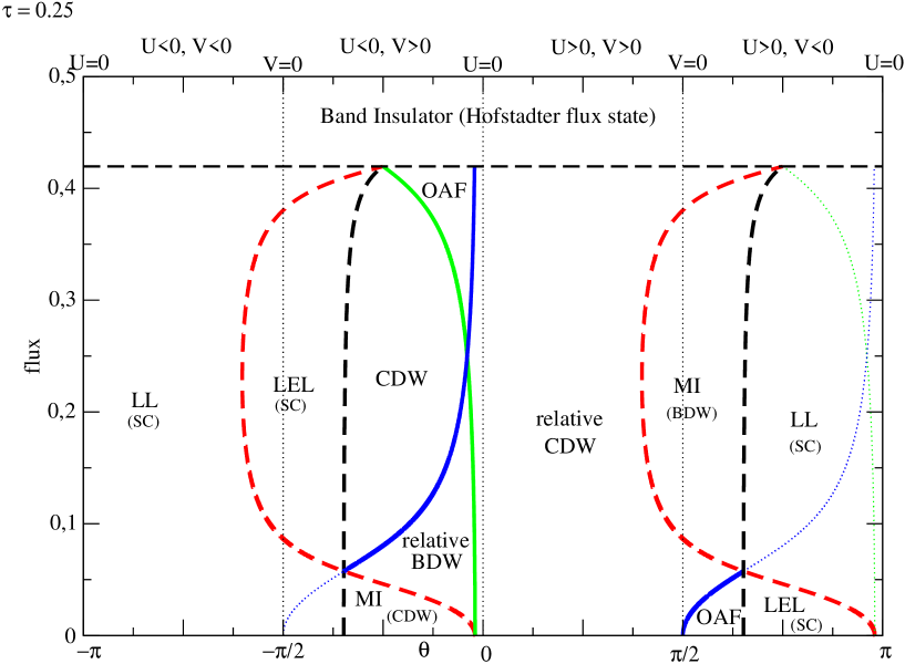
Figure 3: The weak-coupling phase diagram in the magnetic field. We plot the flux along the vertical axis and the angle $\theta$ (defined as $\theta=\tan^{-1}U/2V$) along the horizontal axis. As the phases depend on the signs of the interaction parameters, they are indicated at the top of the diagram. Ordered phases are illustrated pictorially in Fig. 1. The corresponding order parameters are listed in Table 1. The disordered phases are characterized by dominant correlations (indicated in parentheses). For large values of the flux ($\sin^{2}\pi f>1-\tau^{2}$), there is a band gap in the non-interacting picture. The thick solid lines (blue and green online) represent $U(1)$ Gaussian transitions between mutually dual ground states with long-range order, and the thick dotted lines (black and red online) are Berezinski-Kosterlitz-Thouless phase transitions corresponding to opening of a gap in one of the sectors.

Gaussian transitions occur in two domains of the phase diagram: (i) for repulsive intrachain interaction ($V>0$) and weak attractive interchain interaction ($U<0$), and (ii) for $U>0$ and weak $V<0$. In the first case (i), at zero flux the system is a MI. The dominant (longest-range) correlation turns out to be that of the $2k_{F}$ component of the total charge density (hence the label “(CDW)” in Fig. 3; see Section III.4 for details on dominant correlations). As the flux is increased, the system becomes a relative BDW (via the BKT transition where a gap opens in the “relative” sector of the effective theory). Further increase of $f$ drives the system through the $U(1)$ transition to a CDW phase. At larger values of the flux (approaching the band gap limit) values of flux, the system eventually becomes an OAF, again through the Gaussian transition.

The second transition (ii) occurs at small values of the flux. The zero-field ground state is an OAF. As we turn on the flux, the system undergoes a $U(1)$ transition towards a relative CDW state. Further increase of the flux results in closing of the gap in the relative sector (via the BKT transition) and the system becomes a MI, but now the dominant correlation is that of the $2k_{F}$ component of the transverse bond density, labeled by “(BDW)”.

This latter transition turns out to be reentrant. As the flux is further increased the system returns (again via the BKT transition) back to the relative CDW state. There is another example of a reentrant transition in the phase diagram, for $U<0$ and small $V$ the zero-field ground state is a Luttinger Liquid, which once subjected to the external field first becomes a LEL by opening a gap in the “relative” sector, and then at higher field comes back to the LL state in which the most singular fluctuations are those of the pairing operator at momentum $\pi-2k_{F}$. In the LEL phase the “relative” sector is gapped and the “charge” sector is characterized by the dominant correlation of the pairing operator at zero momentum.

Finally there is a large part of the phase diagram which is robust against the application of the external field. When both inter- and intra-chain interactions are attractive, the LL (that is the zero-field ground state) is mostly unaffected by the field. More interesting is the situation when both interactions are repulsive. The zero-field ground state is the relative CDW. It turns out that this long-range order survives under the application of the field (except possibly for the transition to the MI for weak $V$ discussed above).

II.3 Commensurate-Incommensurate transition

The above phase diagram breaks down if the parameter $h=[\sin^{2}(\pi f)+\tau^{2}]^{1/2}$, which in the noninteracting case determines the splitting between the Fermi momenta of different bands, is too small (see Sections III and IV). Then, the part of the phase diagram that corresponds to attractive inter-chain interaction $U<0$ acquires additional ordered phases. This is the result of additional inter-band scattering processes that at larger $h$ violate momentum conservation in the low energy effective theory (based on the two-band description). The latter issue reveals the dichotomy between the two starting points already mentioned in the Introduction: chain basis versus band basis. If one starts with a solution (however complete) for two independent chains and then tries to take into account the inter-chain hopping (as well as the flux) in perturbation theory, then the processes mentioned above are present in the theory from the beginning. In the case when these processes generate a gap in the spectrum of relative degrees of freedom, a finite splitting of the Fermi momenta would not take place unless the parameter $h$ exceeds its critical value comparable with the gap. This is the well-known commensurate-incommensurate transition.boz As the parameter $h$ increases further, the “two-chain” approach fails because renormalization of the parameters of the theory becomes sizable at sufficiently large $h$. At that point one would be forced to start with the exact, two-band single-particle spectrum of the ladder. However, this would seemingly neglect the processes in question as they appear to violate momentum conservation.

In Section IV we discuss the relation between the two approaches to ladder problems and show that if one uses either approach properly, then the final result is independent of the starting point, as should be expected. The new phases at $U<0$ naturally emerge through the commensurate-incommensurate transition.boz

We shall also show that, regardless of the starting point, some properties of the system are not accessible within the effective low energy theory. The quantity in question is the diamagnetic (or persistent) current, which turns out not to be an infra-red property. All electrons participate in this current. In particular, the curvature of the single-particle spectrum at the Fermi points becomes important, so that linearization of the spectrum, being the usual prerequisite in the derivation of any effective low-energy theory, completely destroys this effect. Consequently, within the bosonization approach in the context of the fermion ladder, it is impossible to describe the analog of the Meissner effect that can be seen in bosonic ladders.og01 Details are presented in section IV.

III Low energy effective theory: Band basis

In this Section we derive the effective low energy theory for the model (1) taking the exact single particle spectrum as our starting point. As mentioned above, there exists an alternative approach, which starts with disconnected (but interacting) chains. The relation between the two will be discussed in the next Section.

Figure 4: Possible types of the single-particle spectrum as a function of in-chain momentum. For any given $\tau$, increasing the flux will eventually open a band-gap in the non-interacting spectrum. Close to this transition one of the two bands is almost empty while the other is almost full. At this point, curvature effects of the spectrum become important; these are beyond the scope of this paper.

III.1 Single-particle spectrum

The single-particle part of the Hamiltonian (1) can be diagonalized by the unitary transformation

$$c_{1}(k) = u_{k}\alpha_{k}+v_{k}\beta_{k},$$

$$c_{2}(k) = v_{k}\alpha_{k}-u_{k}\beta_{k}$$ (3)

where the “coherence factors” $u_{k},v_{k}$ [which are positive as the signs are written explicitly in Eq. (3)] are given by (if not stated otherwise, in this section we will measure the momentum $k$ in units of the inverse longitudinal lattice spacing, $1/a$)

$$u^{2}_{k} = \frac{1}{2}\left[1-\frac{\sin k\sin\pi f}{\sqrt{\sin^{2}k\sin^{2}\pi f+\tau^{2}}}\right]$$

$$v^{2}_{k} = \frac{1}{2}\left[1+\frac{\sin k\sin\pi f}{\sqrt{\sin^{2}k\sin^{2}\pi f+\tau^{2}}}\right].$$ (4)

The resulting single-particle Hamiltonian describes two bands

$$H_{0}=\sum_{k}\left[\epsilon_{\alpha}\alpha_{k}^{\dagger}\alpha_{k}+\epsilon_{\beta}\beta_{k}^{\dagger}\beta_{k}\right],$$

with the spectrum

$$\epsilon_{\alpha(\beta)}=-2t_{0}\left[\cos k\cos\pi f\pm\sqrt{\sin^{2}k\sin^{2}\pi f+\tau^{2}}\right].$$ (5)

In the absense of the flux the coherence factors are independent of momentum ($u^{2}=v^{2}=1/2$) and the Hamiltonian $H_{0}$ consists of the usual symmetric and antisymmetric bands each with the cosine spectrum, split by $2t_{\perp}$.

In the presence of the flux the spectrum can take one of the four typical shapes depending on the value of $\tau$ and the flux. These are illustrated in Fig. 4. For completeness we include a detailed discussion of the properties of the spectrum as a function of flux and interchain hopping in Appendix B.

The half-filled ladder is characterized by zero chemical potential. When the spectrum (5) takes the form depicted in the two bottom graphs in Fig. 4, the system at $\mu=0$ is a band insulator. In that case interaction effects (as well as the external field) are not expected to drastically change the nature of the ground state of the non-interacting system. We will not discuss that case in the present paper.

The top two graphs in Fig. 4 describe the “metallic” phase of the non-interacting system. In this case at half filling both bands are partially filled and each band is characterized by its own Fermi momentum $k_{F}^{\alpha(\beta)}$ satisfying $k_{F}^{\alpha}+k_{F}^{\beta}=\pi$. In what follows we will use the notation $k_{F}\equiv k_{F}^{\alpha}$ (so that $k_{F}^{\beta}=\pi-k_{F}$) with

$$\cos k_{F}=\sqrt{\sin^{2}\pi f+\tau^{2}}.$$ (6)

In the presence of the magnetic flux there exists a finite diamagnetic current in the ground state of the system. The current operator along the oriented link between sites $n$ and $n+1$ of the chain $\sigma$ is

$$j_{n,\sigma}=-it_{0}\left(e^{i\pi f\sigma}c_{n,\sigma}^{\dagger}c_{n+1,\sigma}-h.c.\right).$$ (7)

This current flows in opposite directions on the two legs of the ladder, so that the total current $j_{tot}=j_{n,+}+j_{n,-}$ will have zero expectation value, while the expectation value of the relative current $j_{rel}=j_{n,+}-j_{n,-}$ (in the absence of interaction) is given by

$$\langle j_{rel}\rangle=-2t_{0}\sin\pi f\int\frac{dk}{2\pi}\Bigg{\{}\cos k\left[n_{\alpha}(k)+n_{\beta}(k)\right]$$

$$\quad\quad\quad\quad\quad\quad-\frac{\sin^{2}k\cos\pi f\left[n_{\alpha}(k)-n_{\beta}(k)\right]}{\sqrt{\sin^{2}k\sin^{2}\pi f+\tau^{2}}}\Bigg{\}},$$ (8)

where $n_{\alpha(\beta)}(k)=\langle c_{\alpha(\beta)}^{\dagger}(k)c_{\alpha(\beta)}(k)\rangle$ are the occupation numbers of the two bands. The current (8) is a periodic function of the flux with a period $\Delta f=1$. In Fig 5 we plot the flux dependence of $\langle j_{rel}\rangle$ within a single period. Notice that the current changes its sign under transformation $f\to\pi-f$; at $f=1/2$ $\langle j_{\rm rel}\rangle=0$ due to the recovery of time reversal symmetry at this point.

Figure 5: Diamagnetic current as a function of flux in the absence of interaction. Only one period in $f$ is shown. The cusps correspond to the band gap opening.

In the limit $\tau\to 0$, when the ladder decouples into two completely disconnected chains, the appearance of the flux in the Hamiltonian (1) is a gauge artifact. Indeed, a careful evaluation of the integral in Eq. (8) will show that $\langle j_{rel}\rangle=0$ at $\tau=0$. Expanding Eq. (8) for small $f,\tau\ll 1$ and recovering the dependence on the lattice spacing $a$, one finds that

$$\langle j_{rel}\rangle=\frac{v_{F}}{3a}f\tau^{2}\left[1+O(f^{2},\tau^{2})\right].$$ (9)

Despite being small in this limit, the diamagnetic current is not an infra-red phenomenon. Its dependence on $\tau$ is apparently the effect of a finite curvature of the single-particle spectrum. Notice, that as seen from Fig 5, $\langle j_{\rm rel}\rangle$ is non-zero even in the insulating phase. Thus the current is a non-universal quantity contributed by all electrons and not only those in the vicinity of the Fermi points. Consequently, effects related to such a persistent current can not be addressed in terms of any Lorentz-invariant effective low-energy theory (we will further comment on this issue in Section IV). Thus, at present we are unable to calculate the effect of the interaction on the diamagnetic current. However, it is clear that even in the presence of interaction the current will still persist and all the correlation-related phenomena discussed in this paper will coexist with it.

III.2 Interaction Hamiltonian

Now we are going to apply the standard rules of Abelian bosonizationboz ; gia to derive the effective low-energy theory. First, we will assume that the Fermi energy is sufficiently far from the bottom of the $\beta$-band. Then we linearize the two-band spectrum Eq. (5) in the vicinity of the four Fermi points, $\pm k^{\alpha}_{F}$ and $\pm k^{\beta}_{F}$. The associated low-energy degrees of freedom are described in terms of smoothly varying chiral (right and left) fermionic fields, $R_{\alpha(\beta)}(x)$ and $L_{\alpha(\beta)}(x)$. This defines the continuum limit of the model in which the non-interacting part of the lattice Hamiltonian, including both the inter-chain hopping and the coupling to the flux, transforms to the kinetic energy of the chiral particles:

$$H_{0}=-iv_{F}\sum\limits_{\nu=\alpha,\beta}\int dx\left(R_{\nu}^{\dagger}\partial_{x}R_{\nu}-L_{\nu}^{\dagger}\partial_{x}L_{\nu}\right),$$

where $v_{F}=2t_{0}a\sin k_{F}/\cos\pi f$ is the Fermi velocity which at half filling is the same for both bands.

Specializing to the vicinity of the four Fermi points in the coherence factors Eqs. (4) we find the low-energy correspondence between the original lattice operators $c_{i,\sigma}$ and the chiral fields $R_{\nu}$ and $L_{\nu}$. Then, the interaction terms in the model (1) become

$${H}_{int}\approx a\sum\limits_{i}\Bigg{\{}g_{1}\left(:J_{R\alpha}J_{L\alpha}:+:J_{R\beta}J_{L\beta}:\right)+g_{2}\left(:J_{R\alpha}J_{R\beta}:+:J_{L\alpha}J_{L\beta}:\right)+g_{3}\left(:J_{R\alpha}J_{L\beta}:+:J_{L\alpha}J_{R\beta}:\right)$$

$$\quad\quad\quad\quad\quad+g_{4}\left(:R_{\alpha}^{\dagger}L_{\alpha}R_{\beta}^{\dagger}L_{\beta}:+:L_{\alpha}^{\dagger}R_{\alpha}L_{\beta}^{\dagger}R_{\beta}:\right)-g_{5}\left(:R_{\alpha}^{\dagger}L_{\alpha}^{\dagger}R_{\beta}L_{\beta}:+:R_{\alpha}L_{\alpha}R_{\beta}^{\dagger}L_{\beta}^{\dagger}:\right)+$$

$$\quad\quad\quad\quad\quad+g_{6}\left(:R_{\alpha}^{\dagger}(x_{i})R_{\alpha}^{\dagger}(x_{i+1})L_{\beta}(x_{i})L_{\beta}(x_{i+1}):+:R_{\alpha}(x_{i})R_{\alpha}(x_{i+1})L_{\beta}^{\dagger}(x_{i})L_{\beta}^{\dagger}(x_{i+1}):\right)+$$

$$\quad\quad\quad\quad\quad+g_{6}\left(:L_{\alpha}^{\dagger}(x_{i})L_{\alpha}^{\dagger}(x_{i+1})R_{\beta}(x_{i})R_{\beta}(x_{i+1}):+:L_{\alpha}(x_{i})L_{\alpha}(x_{i+1})R_{\beta}^{\dagger}(x_{i})R_{\beta}^{\dagger}(x_{i+1}):\right)\Bigg{\}}.$$ (10)

where $J_{R\nu}=:R^{\dagger}_{\nu}R_{\nu}:$ and $J_{L\nu}=:L^{\dagger}_{\nu}L_{\nu}:$ are the chiral densities of the right- and left-moving fermions with the band index $\nu$ (the symbol “::” stands for normal ordering).

The first three terms in Eq. (10), characterized by coupling constants $g_{1}$,$g_{2}$ and $g_{3}$, describe the density-density interaction, whereas terms with amplitudes $g_{4}$, $g_{5}$ and $g_{6}$ correspond to the interchain umklapp, interchain back-scattering and in-chain umklapp terms, respectively. Explicit expressions for the $g_{i}$ in terms of the original microscopic theory is given in Appendix A. The coupling constants depend on the interaction constants of the microscopic model (1) and, through the coherence factors Eq. (4), on the external flux. The latter dependence plays an important role because it is responsible for the sequence of phase transitions, described in Section II.2), that are not accessible at $f=0$.

The interaction Hamiltonian $H_{int}$ in Eq. (10) is the most general form of four-fermion interaction in the band representation, consistent with momentum conservation (modulo the reciprocal lattice vector). All other terms contain strongly oscillating exponentials and thus do not contribute to the low-energy theory. In particular, this argument applies to the term

$$g_{7}e^{2i(k_{F}^{\alpha}-k_{F}^{\beta})x}R_{\alpha}^{\dagger}L_{\alpha}L^{\dagger}_{\beta}R_{\beta}+h.c.$$ (11)

Note, that if one starts building the low energy theory approximating the ladder by two uncoupled chains, then the Fermi momenta of the two bands are equal and the above term should be included in Eq. (10). We will discuss this term and the relation between the two approaches to bosonization in ladder models in Section IV. However it is immediately clear, that omitting Eq. (11) from Eq. (10) can only be valid at long distances $|x|\gg|k_{F}^{\alpha}-k_{F}^{\beta}|^{-1}$ or, equivalently, at low energies $|\omega|\ll v_{F}|k_{F}^{\alpha}-k_{F}^{\beta}|$.

Now we bosonize the theory in the standard manner (our conventions are outlined in Appendix C). As usual, the density-density terms (represented in Eq. (10) by $g_{1}$, $g_{2}$, and $g_{3}$) renormalize the Fermi velocities and the scaling dimensions of the vertex operators. Introducing symmetric and antisymmetric combinations of the bosonic fields, $\phi_{\pm}=(\phi_{\alpha}\pm\phi_{\beta})/\sqrt{2}$, we diagonalize the quadratic part of the effective bosonized Hamiltonian. The latter is then represented by two sine-Gordon models defined in the symmetric and antisymmetric sectors which are coupled by the in-chain umklapp term $g_{6}$:

$${\cal H}=\frac{v_{F}^{+}}{2}\left[K_{+}\left(\partial_{x}\theta_{+}\right)^{2}+\frac{1}{K_{+}}\left(\partial_{x}\phi_{+}\right)^{2}\right]-\frac{g_{4}}{2\pi^{2}\alpha_{0}^{2}}\cos\sqrt{8\pi}\phi_{+}$$

$$\quad\quad\quad\quad\quad\quad+\frac{v_{F}^{-}}{2}\left[K_{-}\left(\partial_{x}\theta_{-}\right)^{2}+\frac{1}{K_{-}}\left(\partial_{x}\phi_{-}\right)^{2}\right]+\frac{g_{5}}{2\pi^{2}\alpha_{0}^{2}}\cos\sqrt{8\pi}\theta_{-}-\frac{g_{6}}{\pi^{2}\alpha_{0}^{2}}\cos\sqrt{8\pi}\phi_{+}\cos\sqrt{8\pi}\theta_{-}.$$ (12)

The cosine terms in Eq. (12), when relevant (these are the cases $K_{+}<1$, $K_{-}>1$, respectively), are responsible for a dynamical generation of a mass gap in the corresponding sector and, therefore, for the $U(1)$ phase transitions described in Section II.2. For weak interaction, $|g_{i}|/\pi v_{F}\ll 1$, the “Luttinger liquid” parameters $K_{\pm}$ are close to unity (see Appendix A). Consequently, the cosine terms having scaling dimensions $2K_{+}$ and $2/K_{-}$ in the symmetric and antisymmetric sectors, respectively, are nearly marginal. The $g_{6}$ term that couples the two sectors is therefore strongly irrelevant because of its scaling dimension $2K_{+}+2/K_{-}\sim 4$. The only situation when the $g_{6}$ term may become important is the case when one of the sectors is gapped, while the amplitude of the cosine term in the other sector vanishes, i.e. either $g_{4}=0$ or $g_{5}=0$. In this case the $g_{6}$ term can generate the missing cosine in the Gaussian sector and even make the latter massive. This mechanism was recently discussed in Ref. dtgs01, in the context of the Mott instability of a half-filled fermionic ladder with $U=0$. Since in our model the presence of the $g_{4}$ and $g_{5}$ terms is generic, and the lines $g_{4}=0$ and $g_{5}=0$ characterize the phase boundaries, the only effect of the in-chain ($g_{6}$) Umklapp scattering would be to modify the equations that determine the phase boundaries without changing the topology of the phase diagram. Being interested in the description of distinct phases rather than their precise location, we will ignore the $g_{6}$ term in the remainder of this paper.

Thus the effective low energy theory for our model Eq. (1) consists of two asymptotically decoupled sectors, each being a sine-Gordon model. In the case when a strong-coupling regime developes in either sector, a mass gap gets generated in the spectrum, and semiclassical solutions of the equations of motion describe locking of the bosonic field in one of the infinitely degenerate minima of the cosine potential. Physical quantities evaluated on such solutions may either vanish or acquire a nonzero expectation value. The former would mean that the quantity in question is characterized by exponentially decaying correlations. In contrast, the latter corresponds to long-range correlations. Since local operators of the theory have a multiplicative structure, they can indeed serve as order parameters if gaps are generated in both sectors simultaneously. The multiplicity of the actual values that the order parameter would take on the semiclassical solutions, differing by a period of the cosine potential, determines the degeneracy of the ordered ground state. The latter always appears to be associated with a unit cell doubling and is $Z_{2}$. The complexity of the formulae, relating the four coupling constants in (12) to the two interaction parameters in the original Hamiltonian (1), as well as the magnetic field, leads to a rich phase diagram, as we will now demonstrate using the just outlined strategy.

Table 1: Local operaors in the half-filled ladder

Local	Lattice	Dominant	Bosonized	Ordered
Operator	Definition	Component	Form	Phase
$J_{\perp}$	$-it_{\perp}\left[c_{1}^{\dagger}c_{2}-h.c.\right]$	$\pi$	$\cos\sqrt{2\pi}\phi_{+}\cos\sqrt{2\pi}\theta_{-}$	OAF
$\rho_{-}$	$c_{1}^{\dagger}c_{1}-c_{2}^{\dagger}c_{2}$	$\pi$	$\cos\sqrt{2\pi}\phi_{+}\sin\sqrt{2\pi}\theta_{-}$	Rel. CDW
$\rho_{\|,+}$	$e^{i\pi f}c_{1}^{\dagger}(x_{n})c_{1}(x_{n+1})+e^{-i\pi f}c_{2}^{\dagger}(x_{n})c_{2}(x_{n+1})+h.c.$	$\pi$	$\sin\pi f\cos\sqrt{2\pi}\phi_{+}\cos\sqrt{2\pi}\theta_{-}$	BDW
$\rho_{\|,-}$	$e^{i\pi f}c_{1}^{\dagger}(x_{n})c_{1}(x_{n+1})-e^{-i\pi f}c_{2}^{\dagger}(x_{n})c_{2}(x_{n+1})+h.c.$	$\pi$	$\sin\sqrt{2\pi}\phi_{+}\sin\sqrt{2\pi}\theta_{-}$	Rel. BDW
$\rho_{+}$	$c_{1}^{\dagger}c_{1}+c_{2}^{\dagger}c_{2}$	$\pi$	$\tan\pi f\sin\sqrt{2\pi}\phi_{+}\cos\sqrt{2\pi}\theta_{-}$	CDW
		$2k_{F}$	$\sin\sqrt{2\pi}\phi_{+}\cos\sqrt{2\pi}\phi_{-}$
$\rho_{\perp}$	$c_{1}^{\dagger}c_{2}+c_{2}^{\dagger}c_{1}$	$2k_{F}$	$\cos\sqrt{2\pi}\phi_{+}\sin\sqrt{2\pi}\phi_{-}$
$O_{sc}$	$c_{1}c_{2}$	$\pi-2k_{F}$	$ie^{i\sqrt{2\pi}\theta_{+}}\cos[\sqrt{2\pi}\phi_{-}-(\pi-2k_{F})x]$
		0	$\tan\pi fe^{i\sqrt{2\pi}\theta_{+}}\cos\sqrt{2\pi}\theta_{-}$

III.3 Ordered Phases

As there are four distinct Fermi points in our model, any local operator will contain four dominant Fourier components

$${\cal O}(x_{n}) = {\cal O}_{0}(x)+(-1)^{n}{\cal O}_{\pi}(x)$$

$$+ \cos(2k_{F}x_{n})\left[{\cal O}_{2k_{F}}(x)+(-1)^{n}{\cal O}_{\pi-2k_{F}}(x)\right].$$

Here ${\cal O}_{0}$ is the smooth part of the operator ${\cal O}(x_{n})$ corresponding to characteristic momentum $q\sim 0$; ${\cal O}_{\pi}$ is the staggered part contributed by momenta $q\sim\pi$, which can originate from some inter-band pairing; the components ${\cal O}_{2k_{F}}$ and ${\cal O}_{\pi-2k_{F}}$ can be present due to in-band pairing. At half filling, it is only the staggered part that can acquire an expectation value and serve as an order parameter; however in some of the gapless phases dominant correlations may occur at $2k_{F}$ or $\pi-2k_{F}$ rather than $\pi$.

Local operators of interest in the case of half-filled ladder are listed in Table 1, which includes the microscopic lattice definitions and the bosonized form of the dominant Fourier components. These are given up to multiplicative factors; we preserve, however, prefactors proportional to the magnetic flux to make clear which quantities do not exist in zero field limit. We also indicate the LRO that appears when order parameters (first five operators in the Table 1 – which also correspond to the five “cartoons” in Fig 1) acquire nonzero expectation values.

An interesting observation that can be made from Table 1 is that the OAF and the BDW are both proportional to the same low-energy operator, implying that the two phases coexist. However, the OAF can exist already at zero flux whereas the BDW order parameter is proportional to the flux (at small $f$). This coexistence can be understood by noticing that at $f\neq 0$ the BDW order parameter is defined in a gauge invariant way, i.e. with flux-dependent phase factors explicitly included into its definition [we remind that we have chosen the longitudinal Landau gauge, see Eq. (2)]. As a result, the BDW operator describing dimerization of the two chains with zero relative phase acquires an admixture of the staggered relative current, proportional to the flux at $f\ll 1$. This admixture actually represents the longitudinal part of the OAF order parameter (which is identical to $J_{\perp}$ by current conservation). The very appearance of such an admixture is a consequence of the explicit breakdown of time reversal symmetry, caused by the external flux, which is superimposed on the spontaneous breakdown of this symmetry in the OAF phase.

Another ordering in which the flux plays a crucial role is the CDW phase. As already mentioned, the ground state of the ladder at $f=0$ and not too small $\tau$ does not display this type of LRO as the interchain hopping tends to prevent double occupancy of the rungs. It is a curious fact that under application of the flux this state can be recovered due to a similar, although more subtle, admixture with a staggered flux phase. Indeed, the bosonized low-energy projection of the operator $\rho_{+}$ has the form $fJ_{\rm diag}$, where the operator

$$J_{\rm diag}\sim i(-1)^{n}\sum_{\sigma}\sigma\left(c_{n,\sigma}^{\dagger}c_{n+1,-\sigma}-h.c.\right),$$ (13)

represents an order parameter for an OAF state with local currents effectively flowing across the diagonals of the plaquettes.ner The scalar nature of the CDW under time reversal is not violated for the reason already mentioned in the preceeding paragraph.

Let us now turn to the derivation of the phase diagram. For the cosine terms to become relevant and generate a gap in the spectrum, the “Luttinger liquid” parameters $K_{+}$ and $K_{-}$ should be smaller and larger than $1$, respectively. According to the definition of $K_{\pm}$, Eqs.(41), this translates into the following conditions on the parameters of the theory:

$$g_{1}+g_{3}>0;\quad g_{1}-g_{3}<0.$$ (14)

Strictly speaking, these conditions are valid only to first order in the Kosterlitz-Thouless RG equations. When the couplings $g_{i}~{}(i=1,3,4,5)$ are all of the same order, there are important renormalizations of the parameters $K_{\pm}$ emerging in the second-orderboz . This means that the exact positions of the phase boundaries depend also on $g_{4}$ and $g_{5}$. These corrections, however, do not cause qualitative changes in the overall phase diagram and can therefore be neglected in the leading order. For this reason, when drawing conclusions on relevance or irrelevance of various perturbations, we will resort to an estimation of their Gaussian scaling dimension.

In the effective Hamiltonian (12) there are two cosine terms with amplitudes $g_{4}$ and $g_{5}$. Both terms have the same period in their respective variables that defines the values of the fields $\phi_{+}$ and $\theta_{-}$ for any semiclassical solution. Depending on the sign of $g_{4}$ the field $\phi_{+}$ may take one of the two possible sets of values, $\varphi_{0}=n\sqrt{\pi/2},$ or $\varphi_{\pi}=\sqrt{\pi/8}+n\sqrt{\pi/2}$ $(n=0,\pm 1,\ldots)$. Similarly, $\theta_{-}$ may take one of the above values depending on the sign of $g_{5}$. Consequently there are four possible ordered phases.

(i) If both $g_{4}$ and $g_{5}$ are negative, then the semiclassical solutions are $\phi_{+}=\varphi_{\pi}$ and $\theta_{-}=\varphi_{0}$. Of all the operators listed in Table 1 only the staggered component of the total charge density $\rho^{(s)}_{+}$ has a non-zero expectation value on the above solution. Therefore, the conditions $g_{4(5)}<0$ define the charge density wave (CDW). This phase exists only in the presence of the magnetic field, which mixes it up with an OAF phase, as explained previously.

(ii) For $g_{4}>0$ and $g_{5}<0$ we find the orbital antiferromagnet (OAF), since now $\phi_{+}=\theta_{-}=\varphi_{0}$ and the staggered component of the inter-chain current $J_{\perp}$ gains the expectation value. In contrast to the quarter-filled case us , the OAF phase exists even in the absence of the magnetic field.ner ; boz We will clarify this issue in Sec. V. At $f\neq 0$ the OAF coexists with BDW, as we already mentioned.

(iii) When both interaction constants are positive the staggered component of the relative charge density $\rho^{(s)}_{-}$ has an expectation value (since in this case $\phi_{+}=\varphi_{0}$ and $\theta_{-}=\varphi_{\pi}$). We call the corresponding ordered phase a relative charge density wave (Relative CDW). The magnetic field has little effect on this phase except for the exact location of the phase boundary on the phase diagram, which is beyond the scope of this paper.

(iv) Finally, if $g_{4}<0$ and $g_{5}>0$ then $\phi_{+}=\theta_{-}=\varphi_{\pi}$ and the staggered component of the relative longitudinal bond density $\rho^{(s)}_{\|,-}$ acquires a non-zero expectation value yielding the relative bond density wave (Relative BDW). Although the operator $\rho^{(s)}_{\|,-}$ (and therefore its expectation value) does not vanish in the absense of the magnetic field the relative BDW does not exist at $f=0$ (see Fig. 3) since the two conditions $g_{4}<0$ and $g_{5}>0$ can be resolved only when $f>0$.

All above long-range ordered states break spontaneously translational symmetry of the underlying lattice (period doubling) and thus are doubly degenerate. Topological excitations in these phases ($Z_{2}$-kinks) carry unit charge $Q=1$, as opposed to fractional charge $Q=1/2$ in the quarter-filled case. This follows from the definition of the fermionic number carried by a single kink,

$$Q = \sum_{\nu=\alpha,\beta}\int_{-\infty}^{\infty}dx~{}\left[J_{R\nu}(x)+J_{L\nu}(x)\right]$$ (15)

$$= \sqrt{\frac{2}{\pi}}\int_{-\infty}^{\infty}dx~{}\partial_{x}\phi_{+}(x)$$

and the fact that each kink interpolates between the vacuum values of the field $\phi_{+}$ at $x\to\pm\infty$ that differ by a period of the cosine potential, equal to $\sqrt{\pi/2}$.

III.4 Non-ordered phases

In the previous subsection we have discussed the ordered phases occuring under the conditions Eq. (14), i.e. when both sectors in the effective Hamiltonian (12) acquire gaps. In all other cases there exist gapless excitations. These are characterized by correlation functions that at large distances decay as a power law

$$\langle\mathcal{O}(x)\mathcal{O}(0)\rangle\sim 1/x^{d},$$

where $d$ is the scaling dimension of the operator $\mathcal{O}$. Correlations with slowest decay are usually referred to as dominant. In the phase diagram Fig. 3 we categorize the gapless phases according to their dominant correlations, indicating the corresponding order parameter in parentheses. In this subsection we briefly describe such phases.

If the conditions Eq. (14) are reversed and $K_{+}>1$, $K_{-}<1$, then both sectors are gapless and the system is a Luttinger liquid. In this case the dominant correlation function is that of the pairing operator $O_{sc}$ at wavevector $\pi-2k_{F}$:

$$\langle O_{sc}^{\dagger}(\tau,x)O_{sc}(0)\rangle\sim\frac{\cos[(\pi-2k_{F})x/a]}{|v_{+}\tau-ix|^{2/K_{+}}|v_{-}\tau-ix|^{K_{-}}}.$$ (16)

There are two other cases when only one of the conditions Eq. (14) is violated. Then only one of the sectors acquires a gap while the other remains gapless:

(i) If $K_{+}<1$, $K_{-}<1$, then the “charge” sector is gapped, but the “relative” sector remains gapless. By formal analogy with the Hubbard model we call this phase a Mott Insulator. In such state, incommensurate density or bond-density correlations with characteristic momentum $2k_{F}\neq\pi$ are dominant. Indeed, depending on the sign of $g_{4}$, either $\cos\sqrt{2\pi}\phi_{+}$ or $\sin\sqrt{2\pi}\phi_{+}$ acquire finite expectation values. Therefore, either the transverse bond density $\rho_{\perp}$ or the $2k_{F}$ part of the total charge density $\rho_{+}$ display slowest algebraic decay of the corresponding correlation function determined by the “relative” sector (see Table 1 for bosonized expressions). So at $g_{4}>0$

$$\langle\rho_{\perp}(\tau,x)\rho_{\perp}(0)\rangle\sim\frac{\cos(2k_{F}x/a)}{|v_{-}\tau-ix|^{K_{-}}}.$$ (17)

If $g_{4}<0$, then Eq. (17) applies to the correlation function of $\rho_{+}$.

(ii) If $K_{+}>1$, $K_{-}>1$, then the “charge” sector is gapless, but the relative sector acquires a gap. By analogy with spin-gap systems, we call such a phase a Luther-Emery liquid.lel Now it is $\theta_{-}$ that takes one of the two semiclassical values depending on the sign of $g_{5}$. It turns out, however, that this phase can only occur when $g_{5}<0$, so that $\langle\cos\sqrt{2\pi}\theta_{-}\rangle\neq 0$, and the dominant correlation is that of the pairing operator at zero momentum (with the power law determined by the “charge” sector)

$$\langle O_{sc}^{\dagger}(\tau,x)O_{sc}(0)\rangle\sim\frac{1}{|v_{+}\tau-ix|^{1/K_{+}}}.$$ (18)

The phase boundaries as a function of $U,V,f,\tau$ can be calculated by solving Eqs.(38g) for when $g_{4}$ or $g_{5}$ is zero, or $K_{+}$ or $K_{-}$ is one. For completeness, these are written in Appendix A. The complete weak-coupling phase diagram is plotted in Figure 3 and was discussed in Section II.2.

IV Low energy effective theory: Chain basis

In this section we briefly review the effective low energy theory that one can derive taking two independent chains as a starting point. Interchain hopping is then taken into account already at the bosonization level similarly to interaction terms. This approach is valid as long as $t_{\perp}\ll v_{F}(f)a$, where $v_{F}(f)$ is the renormalized velocity (see below). In the absence of the magnetic field the chain-basis description of the spinless ladder has been widely used in literature.boz ; gia Skipping inessential details, below we will give a brief review which will help to analyze differences between the two approaches and further clarify the role of the magnetic flux.

In the chain-basis approach, one starts by linearizing the fermion dispersion on each chain in the vicinity of the two Fermi points, $\pm k_{F}=\pm\pi/2$, defines chiral fermion fields, and then expresses the inter-chain hopping in terms of these fields. On the lattice, the magnetic field was introduced in the Hamiltonian (1) via the Peierls substitution Eq. (2). Here it is convenient to split the phase exponential in Eq. (2) into its real and imaginary part. The real part contributes to the renormalization of the Fermi velocity, $v_{F}\to v_{F}(f)=v_{F}\cos(\pi f)$, which is of minor importance as long as $f$ is not too close to $1/2$. The imaginary part can be written in terms of the densities of the left and right particles, so that the single-particle perturbation to free chiral fermions is of the form:

$${\cal H}_{1}(x)=-{\bf h}_{R}\cdot{\bf J}_{R}-{\bf h}_{L}\cdot{\bf J}_{L}$$ (19)

where the chiral densities (vector currents) are defined as

$${\bf J}_{R}=\frac{1}{2}R^{\dagger}_{\alpha}\mathbf{\sigma}_{\alpha\beta}R_{\beta},\quad\quad{\bf J}_{L}=\frac{1}{2}L^{\dagger}_{\alpha}\mathbf{\sigma}_{\alpha\beta}L_{\beta}.$$ (20)

Here $\sigma^{a}~{}(a=x,y,z)$ are the Pauli matrices and $\alpha$ and $\beta$ are the chain indices. In Eq. (19) the vector currents appear to be coupled to the effective chiral “magnetic” fields

$${\bf h}_{R}=(h_{\perp},0,-h_{\|}),\quad\quad{\bf h}_{L}=(h_{\perp},0,h_{\|}).$$ (21)

with

$$h_{\|}=4t_{0}\sin(\pi f),\quad h_{\perp}=2t_{\perp}.$$

Bosonizing Eq. (19) directly one can find

$${\cal H}_{1}=\frac{h_{\perp}}{\pi\alpha_{0}}\cos\sqrt{2\pi}\phi_{-}\sin\sqrt{2\pi}\theta_{-}-h_{\|}\sqrt{\frac{2}{\pi}}\partial_{x}\theta_{-}.$$ (22)

Notice that only the relative field, $\phi_{-}=(\phi_{1}-\phi_{2})/\sqrt{2}$ and its dual, $\theta_{-}=(\theta_{1}-\theta_{2})/\sqrt{2}$ appear in Eq. (22) since we are discussing inter-chain processes. To avoid confusion, we remind that here $\phi_{-}$ and $\theta_{-}$ are the differences between the corresponding bosonic fields defined at each chain. The remainder of the Hamiltonian in the relative sector originates from the kinetic term and the interaction, so the total Hamiltonian has the form

$$\mathcal{H}_{-}=\mathcal{H}_{G}+\mathcal{H}_{SG}+\mathcal{H}_{1},$$ (23)

where $\mathcal{H}_{G}$ is the Gaussian model with the interaction parameter $K$ expressed in terms of $g_{s}=(4V-U)a$ in the standard way, Eq. (41), and $\mathcal{H}_{SG}\propto U\cos\sqrt{8\pi}\phi_{-}$ is the sine-Gordon term.

The last term in Eq. (23) ${\cal H}_{1}$ is the sum of a nonlocal vertex operator and a derivative of the dual field $\theta_{-}$. The latter appears only in the presence of the magnetic field and may be interpreted as the bosonized version of the Lorentz-invariant current $\tilde{j}\propto J^{z}_{R}-J^{z}_{L}$. It is important to realize, however, that this is not the physical relative current already discussed in Section III.1. Moreover, $\tilde{j}$ appears not to be gauge-invariant: its expectation value in the ground state of the non-interacting system is non-zero even in the absence of inter-chain hopping. In what follows we demonstrate that, physically, ${\cal H}_{1}$ [Eq. (22)] describes the splitting of the two Fermi points in the chain basis into the four Fermi points introduced in Section III.1.

Treating Eq. (23) presents certain difficulties related to the non-local nature of the perturbation (22). Global rotations of the quantization axis for the Abelian bosonization, which proved to be efficient at $f=0$ (see Refs. nlk93, ; boz, ), are not helpful here because of the more complicated structure of ${\cal H}_{1}$. Let us therefore perform a chiral rotation which makes the “magnetic” fields ${\bf h}_{R}$ and ${\bf h}_{L}$ antiparallel and aligned along the $z$-axis:

$${\bf h^{\prime}}_{R}=(0,0,-h),\quad\quad{\bf h^{\prime}}_{L}=(0,0,h),$$ (24)

where $h^{2}=h_{\perp}^{2}+h_{\|}^{2}$. This simplifies the bosonic form Eq. (22) which now contains only the derivative term

$${\cal H}_{1}=-h\sqrt{\frac{2}{\pi}}\partial_{x}\theta_{-}.$$ (25)

To achive this result we need to rotate the right field by $\omega$ and the left field by $-\omega$ about the $y$ axis where $\tan\omega=h_{\perp}/h_{\|}$ (so that $\omega=\pi/2$ corresponds to the absence of flux). In terms of the fermion operators this chiral $SU(2)$ rotation can be written as

$$R_{\alpha}\to\left[e^{i\omega\sigma_{y}/2}\right]_{\alpha\beta}R_{\beta},\quad L_{\alpha}\to\left[e^{-i\omega\sigma_{y}/2}\right]_{\alpha\beta}L_{\beta}.$$ (26)

The transformation (26) is closely related to the Bogolyubov transformation Eq. (3) used to diagonalize the single-particle Hamiltonian in the band approach. Below we analyze the relation between the two in detail.

While the rotation (26) simplifies the single-particle terms in the Hamiltonian, the interaction terms undergo a nontrivial modification. Since the rotation involves only “relative” fields, the “charge” sector is left unaffected and is a usual sine-Gordon model, with a cosine term $\propto-U\cos\sqrt{8\pi}\Phi_{+}$. For the rest of this Section we will assume this interaction to be strong enough to generate the gap in the “charge” sector and focus on the “relative” degrees of freedom. The Hamiltonian density describing the “relative” sector transforms to

$${\cal H}_{-}=\frac{v_{-}}{2}\left[K_{-}\Pi_{-}^{2}+\frac{1}{K_{-}}(\partial_{x}\phi_{-})^{2}\right]-\frac{g_{\phi}}{(\pi\alpha_{0})^{2}}\cos\sqrt{8\pi}\phi_{-}-\frac{g_{\theta}}{(\pi\alpha_{0})^{2}}\cos\sqrt{8\pi}\theta_{-}-h\sqrt{\frac{2}{\pi}}\partial_{x}\theta_{-}$$

$$\quad\quad\quad\quad\quad\quad\quad\quad+\frac{g_{r}}{\pi^{3/2}\alpha_{0}}\left[(\partial_{x}\phi^{R}_{-})\sin\sqrt{8\pi}\phi_{-}^{L}+(\partial_{x}\phi^{L}_{-})\sin\sqrt{8\pi}\phi_{-}^{R}\right],$$ (27)

with all the coupling constants listed in the Appendix A. In Eq. (27) the relative sector represents a $Z_{4}$ modelwieg ; giaschulz modified by the $g_{r}$ term. Notice that the latter has zero conformal spin and scaling dimension

$$d_{r}=1+\frac{1}{2}\left(K_{-}+\frac{1}{K_{-}}\right)>2$$

for any $K_{-}\neq 1$. Thus this term is irrelevant in the RG sense.Thus, as for the ladder in the absence of the magnetic flux, the effective model appears to be two-cosine $Z_{4}$ model with a topological term. The only but important difference with the $f=0$ case is a nontrivial dependence of the coupling constants on the ratio $\tau/\sin\pi f$ through the rotation angle $\omega$.

At $h=0$, the $Z_{4}$ model in Eq. (27) always displays a strong-coupling regime in the infrared limit accompanied by a dynamical generation of a mass gap. If $K<1$, then $g_{\phi}$ term is relevant while the term $g_{\theta}$ with the dual field is irrelevant. Hence the field $\phi_{-}$ gets locked and the term $h\partial_{x}\theta_{-}$ has no effect on the corresponding long range order. In particular if $g_{\phi}>0$, then the ground state is the relative CDW, which becomes the OAF when $g_{\phi}$ changes sign (e.g. due to the variation of the flux). However, locking of the field $\phi_{-}$ does not prevent the gradient of the dual field $\partial_{x}\theta_{-}$ to acquire a finite expectation value and, thus, produce a finite splitting of the Fermi momenta proportional to $h$ (see the discussion below).

In the opposite case $K>1$, the $g_{\theta}$ term is relevant and leads to locking of the dual field $\theta_{-}$. As long as $h$ remains smaller that the gap generated in the “relative” sector, the ground state is the commensurate CDW, which replaces the MI shown in the phase diagram 3. In this phase the vacuum value of $\theta_{-}$ resides in one of the minima of the cosine potential and remains spatially uniform, implying that $\langle\partial_{x}\theta_{-}\rangle=0$. Thus no band splitting occurs in this regime reflecting the fact that the chains remain effectively decoupled. This is a manifestation of the Anderson confinement and - the in-chain correlations suppress single-particle tunneling between the chains in the low-energy limit. Consequently the flux has little effect on this phase.

The situation changes when $h$ reaches a critical value $h_{c}$ proportional to the mass gap

$$h_{c}\sim\Delta_{s}/v_{F}a\sim\exp(-2\pi v_{F}/|g_{s}|)\ll 1\quad(g_{s}<0).$$ (28)

At this point a commensurate-incommensurate transition takes place, the long-range order disapears and a finite gradient $\langle\partial_{x}\theta_{s}\rangle$ emerges in the ground state, following the universal square-root increase $\sim\sqrt{h-h_{c}}$ slightly above the threshold.boz The commensurate CDW gets replaced by the MI phase with incommensurate leading correlations. The appearance of a finite average $\langle\partial_{x}\theta_{s}\rangle$ indicates that the two doubly degenerate Fermi points, characterizing the bare-particle spectrum in the chain basis, are getting split.

Note, that the commensurate-incommensurate transition can be seen within the band basis approach if one takes into account an additional interaction process mentioned previously in Eq. (11), which is usually disregarded since formally it does not conserve momentum. The term is the interband backscattering

$$R_{\alpha}^{\dagger}R_{\beta}L_{\beta}^{\dagger}L_{\alpha}+h.c.$$ (29)

In bosonized form this can be written as

$$\frac{g_{7}}{(2\pi\alpha_{0})^{2}}\cos(\sqrt{8\pi}\phi_{-}+2hx)$$ (30)

where the relation between $g_{7}$ and the microscopic parameters of the model is given in Eq. (38g). Adding this term to the bosonic two-band Hamiltonian (12) and making a shift

$$\phi_{-}\rightarrow\phi_{-}-hx/\sqrt{2\pi}$$ (31)

one transforms the relative part of the Hamiltonian (12) to the form identical to the $Z_{4}$ part in Eq. (27) (up to duality transformation $\phi_{-}\leftrightarrow\theta_{-}$). The above analysis holds identically for this representation. While the case $h\ll 1$ may be easier to describe within the chain approach, the band picture should always give the correct result. In particular, to find the above CDW order, one has to notice that for sufficiently small $h$ when $\langle\cos\sqrt{2\pi}\phi_{-}\rangle\neq 0$, the $2k_{F}$ component of the CDW order parameter listed in Table 1 acquires a nonzero expectation value (now $2k_{F}=\pi$), and the MI phase in the bottom left of the phase diagram 3 becomes a CDW phase with long range order.

V Strong Coupling

In this Section we discuss the behavior of the system in the strong-coupling limit, $|U|,|V|\gg t_{0}$. In the atomic limit when hopping is completely neglected ($t_{0}=t_{\perp}=0$), the particles are localized on sites, and there are four possible ground states. Which state has the lowest energy is determined by the signs of the interaction parameters $U$ and $V$: (i) if $U,V>0$, then the ground state is the Relative CDW (the SDW^z in the “spin” language) depicted in Fig. 1; (ii) when $U<0$ and $V>0$ the state is the CDW also shown in Fig. 1; (iii) in the opposite case $U>0$ and $V<0$ all particles fully occupy one chain keeping the other empty; and finally, (iv) when $U,V<0$ we have complete phase separation.

Of the above four ground states the first two are accessible in the weak coupling approach as can be seen from the phase diagram in Fig. 3. The phases (iii) and (iv) do not have the lowest energy when the bandwidth $t_{0}$ is greater or of the same order as $U$ and $V$ and thus have no analog in weak coupling.

To make further links with the weak coupling approach we now need to take into account the hopping terms and the magnetic field. Of the above four cases only the first one needs to be discussed in detail. Indeed, the last two do not appear in weak coupling, while in the case (ii) we have either doubly occupied or empty rungs, so that inter-chain hopping and the flux do not afect the properties of the ground state. This ground state (CDW) was discussed in the previous section (this is the case where $h$ is smaller than the gap, see Eq. (28).

Consider the limit where $U>0$ is the largest scale in the problem. Then we can project out states with doubly occupied rungs. Then at half-filling and at energies well below the local charge gap, there only remain configurations with exactly one fermion per rung. Accordingly, the relative degrees of freedom can be conveniently described in terms of local spin-1/2 variables using the correspondence between two single-fermion states at a given rung $n$ and the eigenstates $|\uparrow\rangle$ and $|\downarrow\rangle$ of the operator $S^{z}_{n}$. The standard Schrieffer-Wolff transformation sw66 leads to the following effective spin-chain model:

$${\cal H}_{eff} = J_{0}\sum_{n}\Big{[}\frac{1}{2}\left(e^{2i\pi f}S_{n}^{+}S_{n+1}^{-}+e^{-2i\pi f}S_{n}^{-}S_{n+1}^{+}\right)$$ (32)

$$\quad\quad+\Delta S_{n}^{z}S_{n+1}^{z}+h_{\perp}S_{n}^{x}\Big{]},$$

where $J_{0}=2t_{0}^{2}/U$ is the exchange constant, $\Delta=(J_{0}+V)/J_{0}$ is the anisotropy parameter, $h_{\perp}=t_{\perp}/J_{0}$ is the transverse field and $f$ is the external flux in the original ladder model. Notice, that the Schrieffer-Wolff transormation leaves the “charge” sector gapped, so that all subsequent analysis pertains to the “relative” sector.

In the spin language, the Relative CDW order parameter (see Table 1) corresponds to the staggered magnetization in the $z$-direction $(-1)^{n}S_{n}^{z}$, while the OAF order parameter is the staggered magnetization in the $y$ direction, $(-1)^{n}S_{n}^{y}$. Magnetization in the $x$ direction corresponds to the transverse bond density. Since the uniform transverse field $h_{\perp}$ breaks the $U(1)$ symmetry of the XXZ chain, the staggered component $(-1)^{n}S_{n}^{x}$ never acquires a non-zero expectation value.

The effective spin model Eq. (32) is not integrable and its general solution remains unknown. Nevertheless, there exist at least three cases where further progress can be made: (a) the case $f=0$ which has been studied previously (see e.g. Ref. cel03, ); (b) the vicinity of the $SU(2)$-symmetric point $\Delta=1$ and $f\ll 1$; and (c) the vicinity of $f=1/2$. In what follows we discuss these three cases.

(a) In the absence of the flux $f=0$ the Hamiltonian (32) becomes equivalent to the transverse field XXZ model. Despite not being integrable, much is known about such models.cel03 Here, we summarize the results for the sake of completeness referring the interested reader to the literature for more details.

First consider the case $V>0$ (so that $\Delta>1$) and the limit $V\gg 2t_{0}^{2}/U$ in which the exchange anisotropy becomes very large, $\Delta\gg 1$. In this case one can retain only the last two terms in (32), so that the Hamiltonian becomes equivalent to the one-dimensional Ising model in a transverse magnetic field. At $h_{\perp}<\Delta/2$ the ground state is the ordered Neel phase with $\langle(-1)^{n}S_{n}^{z}\rangle\neq 0$. This ordering translates to the Relative CDW for the original ladder, in agreement with the weak-coupling picture. However, when $h_{\perp}=\Delta/2$ a $Z_{2}$ (Ising) transition to a disordered phase takes place. This transition is not present in the weak-coupling phase diagram, so we will not discuss it any further.

Now, if $V<0$ but is sufficiently small ($-1<\Delta<1$), then in the absence of $h_{\perp}$ the Hamiltonian (32) corresponds to the critical XXZ model, which has a gapless excitation spectrum and displays dominant antiferromagnetic fluctuations in the $xy$-plane. A non-zero transverse field breaks the $U(1)$ symmetry down to $Z_{2}$ partially polarizing the spins in the $x$-direction, so that $\langle(-1)^{n}S_{n}^{y}\rangle$ develops an expectation value. This is the OAF phase already discussed in connection with the weak-coupling phase diagram.

Finally, if $\Delta<-1$ then the model is the easy axis XXZ ferromagnet with $\langle S_{n}^{z}\rangle\neq 0$. Such a ground state corresponds to the case (iii) above, i.e. all particles localized on one of the chains.

(b) We now consider the case $|\Delta-1|\ll 1$ and $f\ll 1$. In this limit the Hamiltonian (32) can be represented (to lowest order in $f$) in the form

$${\cal H} = J_{0}\sum_{n}\big{\{}\vec{S}_{n}\cdot\vec{S}_{n+1}+(\Delta-1)S_{n}^{z}S_{n+1}^{z}$$ (33)

$$+ h_{\|}(\vec{S}_{n}\times\vec{S}_{n+1})^{z}+h_{\perp}S_{n}^{x}\big{\}},$$

i.e. we have a model of a weakly anisotropic XXZ spin chain in a magnetic field $h_{\perp}=t_{\perp}/J_{0}$ along the $x$ direction, and also perturbed by the term proportional to the $z$-component of the spin-current $({\bf S}_{n}\times{\bf S}_{n+1})^{z}$ with an amplitude proportional to the flux, $h_{\|}=\pi f$. Bosonizing around the $SU(2)$-symmetric point in the standard way,boz one can show that the last two terms in Eq. (33) can be written in the form Eq. (19) with the chiral “magnetic” fields, Eq. (21), renormalized by the new “bandwidth” $J_{0}$. Thus we find that the bosonized form of Eq. (33) has the structure of Eq. (23), where the first two terms $\mathcal{H}_{G}$ and $\mathcal{H}_{SG}$ constitute the Abelian bosonic representation of the $SU(2)$-symmetric Heisenberg model in the scaling limit, with the Lutting parameter and the effective coupling constant renormalized by the weak anisotropy term $|\Delta-1|\propto V$ in Eq. (33).

Notice that the resulting Hamiltonian is basically the same as that obtained at weak coupling in the chain basis (23). Therefore the next step, namely the rotation Eq. (26) and its result Eq. 27, can be performed in exactly the same manner as before. As a result, at least in the region $U>0$, all conclusions drawn at weak coupling also hold true in the strong coupling limit. In particular the region of the phase diagram discussed in the previous Section survivies (up to renormalizations of the phase boundaries) in the strong coupling regime as well.

(c) Finally, we consider the case where flux is close to one half. Here we are close to the transition to a band insulator. This region of the phase diagram can not be well treated in our weak coupling approach. In this sense, the strong coupling arguments compliment the weak coupling picture presented in Section III.

Consider a gauge transformation

$$S_{n}^{+}\rightarrow S_{n}^{+}e^{2i\pi fn},\quad\quad S_{n}^{-}\rightarrow S_{n}^{+}e^{-2i\pi fn},$$ (34)

which transforms the Hamiltonian (32) to

$${\cal H}_{eff} = J_{0}\sum_{n}\Big{[}\frac{1}{2}\left(S_{n}^{+}S_{n+1}^{-}+S_{n}^{-}S_{n+1}^{+}\right)+\Delta S_{n}^{z}S_{n+1}^{z}$$ (35)

$$+h_{\perp}\left(S_{n}^{+}e^{2i\pi fn}+S_{n}^{-}e^{-2i\pi fn}\right)\Big{]}.$$

The model (35) is completely equivalent to Eq. (32) but now the transverse field is non-uniform. The situation significantly simplifies when $|f-1/2|\ll 1$. In the case this field becomes almost staggered and can be directly bosonized (in the region $|\Delta|<1$, i.e $V<0$).boz As a result, Eq. (35) becomes

$$H = \frac{u}{2}\int dx\left[K\Pi^{2}+\frac{1}{K}(\partial_{x}\Phi)^{2}\right]$$

$$+ h_{\perp}\int dx\cos\left[\sqrt{\pi}\Theta(x)-2\pi\left(\frac{1}{2}-f\right)\frac{x}{a}\right],$$

where the Luttinger liquid parameter is given by

$$K=\pi/2(\pi-\cos^{-1}\Delta).$$ (37)

For $f=1/2$, the cosine term is relevant and generates a gap in the spectrum. The resulting ground state is the band insulator and the gap corresponds to that seen already in the single-particle problem in Section III.1. This can be seen from the fact that $\cos(\sqrt{\pi}\Theta)$ (which gains a non-zero expectation value at $f=1/2$) corresponds to the uniform bond density.

As $f$ decreases away from $1/2$, eventually the gap will close via a commensurate-incommensurate transition. The system will now have gapless excitations in the relative sector (i.e as in a MI), in qualitative agreement with the weak coupling phase diagram Fig 3.

Finally, if $V>0$ so that $\Delta>1$ one can still bosonize the Hamiltonian (35), although now there is an extra term proportional to $\cos{\sqrt{16\pi}\Phi}$ which is relevant (formally, this is the case $K<1/2$ which is not captured Eq. (37)). We now have two competing cosine terms in the Hamiltonian, $\cos\sqrt{16\pi}\Phi$ and $\cos[\sqrt{\pi}\Theta(x)-2\pi(1/2-f)x/a]$. The dual field term has the smallest scaling dimension and therefore, when $f=1/2$, determines the character of the ground state. If the flux is decreased, then again the order is destroyed. In this case, however, the other relevant operator in the problem, $\cos\sqrt{16\pi}\Phi$ should at this point acquire a non-zero expectation value. This is the transition between the band-insulator and the relative CDW, again in agreement with Fig 3.

VI Summary

We have investigated a model of interacting spinless fermions hopping on a two-leg ladder in the presence of an external magnetic field at half-filling. Using bosonization techniques, we constructed the effective low energy theory where the coupling constants acquired non-trivial dependence on the external flux. Consequently the flux results in several phase transitions shown in the weak-coupling phase diagram Fig. 3, i.e. BKT transitions between ordered and disordered phases and $U(1)$ transitions between different ordered phases.

Furthermore, we extended our weak-coupling picture by the special consideration of the case of weakly coupled chains at small flux. We solved the corresponding effective theory using the chiral rotation Eq. (26). As a result we described the commensurate-incommensurate transition from the MI phase shown in Fig. 3 at $U<0$ to the CDW. This transition happens when the parameter $\sqrt{\tau^{2}+\sin^{2}\pi f}$ becomes small enough [see Eq. (28)].

The weak coupling analysis is complimented by the strong coupling arguments. In particular we showed that in some cases (in particular, for small flux and small in-chain interaction $V$), that the weak-coupling approach and strong-coupling approach lead to identical low-energy theories.

Finally, we discussed the persistent (diamagnetic) current flowing in the ladder when the external magnetic field is applied. We showed that even in the limit of small $f$ and small $t_{\perp}$, all electrons in the system contribute to this current and therefore it is a non-universal feature which can not be described in the traditional field-theoretic approach. We speculate that it may be an interesting physical quantity to investigate within the non-linear bosonization scheme.nlb

Appendix A Relation between parameters and phase boundaries

Here we list the effective coupling constants for the effective low energy theory and their relation to the microscopic parameters in the original ladder Hamiltonian Eq. (1).

First, we show the parameters of the $g-$ology for the effective interaction Eqs. (10) and (11) in Section III.2:

$$g_{1}=\frac{\cos^{2}\pi f-\tau^{2}}{\sin^{2}\pi f+\tau^{2}}\left[Ua\tan^{2}\pi f+2Va\frac{\tau^{2}}{\cos^{2}\pi f}\right];$$ (38a)

$$g_{2}=Ua+2Va\frac{\tau^{2}}{\cos^{2}\pi f};$$ (38b)

$$g_{3}=2Va+\frac{1}{\sin^{2}\pi f+\tau^{2}}\Bigg{[}\frac{Ua\tau^{2}}{\cos^{2}\pi f}$$ (38c)

$$\quad\quad\quad\quad\quad\quad+2Va(\sin^{2}\pi f-\tau^{2}\tan^{2}\pi f)\Bigg{]};$$

$$g_{4}=g_{2};$$ (38d)

$$g_{5}=g_{1};$$ (38e)

$$g_{6}=\frac{Va}{4}\left(1+\tan^{2}\pi f\frac{\cos^{2}\pi f-\tau^{2}}{\sin^{2}\pi f+\tau^{2}}\right)$$ (38f)

$$g_{7}=-\frac{\tau^{2}}{\cos^{2}\pi f}\Bigg{[}2Va+\frac{Ua-2Va}{\sin^{2}\pi f+\tau^{2}}\Bigg{]}$$ (38g)

The two “Luttinger parameters” are then given by

$$K_{\pm}=\left[\frac{1-(g_{1}\pm g_{3})/4\pi v_{F}^{\pm}}{1+(g_{1}\pm g_{3})/4\pi v_{F}^{\pm}}\right]^{1/2}$$ (39)

The phase boundaries in Fig. 3 (within the accuracy of one-loop renormalization group approach) are given by the following conditions:

$$g_{1}+g_{3}=0 : \frac{U}{2V}=-\frac{2\cos^{2}\pi f-\tau^{2}}{\cos^{2}\pi f}$$

$$g_{1}-g_{3}=0 : \frac{U}{2V}=\frac{\sin^{2}\pi f(2\cos^{2}\pi f-\tau^{2})+\tau^{4}}{\sin^{2}\pi f(\cos^{2}\pi f-\tau^{2})-\tau^{2}}$$

$$g_{4}=0 : \frac{U}{2V}=-\frac{\tau^{2}}{\cos^{2}\pi f}$$

$$g_{5}=0 : \frac{U}{2V}=-\frac{\tau^{2}}{\sin^{2}\pi f}$$ (40)

Notice that the boundaries depend only on the ratio $U/V$.

Finally, we list the effective constants for the effective low energy theory in the “chain basis” Eq. (27)

$$g_{\phi}=\frac{1}{2}\left[2Va\sin^{2}\omega+Ua\cos^{2}\omega\right];$$

$$g_{\theta}=\frac{2Va-Ua}{2}\sin^{2}\omega;$$

$$g_{r}=(2Va-Ua)\sin 2\omega;$$

$$g_{s}=\left[4Va\cos^{2}\omega+Ua(\sin^{2}\omega-\cos^{2}\omega)\right],$$

$$K_{s}=\left[\frac{1-g_{s}/2\pi v_{s}}{1+g_{s}/2\pi v_{s}}\right]^{1/2}.$$ (41)

Appendix B Single Particle Properties

Here we point out trivial properties of the single-particle spectrum (5) for the sake of completeness. The upper band has its absolute minimum at $k=0$ with

$$(\epsilon_{\beta})_{min}=\epsilon_{\beta}(0)=\tau-\cos\pi f.$$ (42)

The lower band has its absolute maximum at $k=\pm\pi$

$$(\epsilon_{\alpha})_{max}=\epsilon_{\alpha}(\pi)=\cos\pi f-\tau.$$ (43)

Thus, if $\cos\pi f<\tau$, the spectrum exhibits a single-particle gap and the non-interacting system is a band insulator at half filling.

Figure 6: The phase diagram of the non-interacting system. The vertical axis is the external flux and the horizontal axis is the ration between inter-chain and in-chain hopping amplitudes. Fig. 4 demonnstrates the four typical shapes of the spectrum corresponding to the four corners in which the phase diagram is separated by the two lines Eq. (45).

If the flux is not too small then there is a non-trivial extremal point $\cos k_{1}=-\cot\pi f\sqrt{\tau^{2}+\sin^{2}\pi f}.$ For the upper band the energy $\epsilon_{\beta}(k_{1})$ has to be compared to the remaining extremum $\epsilon_{\beta}(\pi)$. If $\sin^{2}\pi f>\tau\cos\pi f$ the band acquires a double-well shape as shown in plots II and IV in Fig. 4 and $k_{1}$ turns out to be the absolute maximum for the uper branch of the spectrum, while $k=\pm\pi$ are local minima. For the lower branch of the spectrum and under the same condition, $k_{1}$ is the absolute minimum, while $k=0$ is the local maximum with the energy value

$$\epsilon_{\alpha}(0)=-\tau-\cos\pi f$$ (44)

The two aforementioned conditions, namely,

$$\cos\pi f_{2}=\tau;\quad\quad\sin^{2}\pi f_{1}=\tau\cos\pi f_{1}$$ (45)

define the two boundaries in the phase diagram of the non-interacting system shown in Fig. 6. These two lines separate the phase diagram of the non-interacting system (Fig. 6) into four parts, where the spectrum has one of the four shapes shown in Fig. 4.

Appendix C Bosonization conventions

Here for completeness we define our bosonization conventions. The chiral bosonic fields are introduced via the correspondence

$$\left(R_{\nu}(x),L_{\nu}(x)\right)\to\left(\kappa_{\nu}/\sqrt{2\pi\alpha_{0}}\right)e^{{\pm i\sqrt{4\pi}\phi^{R(L)}_{\nu}}},$$ (46)

$$J_{R\nu}=\partial_{x}\phi_{R\nu}/\sqrt{\pi},\quad J_{L\nu}=\partial_{x}\phi_{L\nu}/\sqrt{\pi}.$$ (47)

Here $\nu=\alpha,\beta$, $\alpha_{0}$ is an ultraviolet cutoff in the bosonic theory, $\kappa_{\nu}$ are Klein factors that ensure proper anticommutation relations between the fermionic fields with different band indices in representation (46). The $\kappa_{\nu}$ satisfy

$$\{\kappa_{\mu},\kappa_{\nu}\}=2\delta_{\mu\nu};\quad\kappa_{\alpha}\kappa_{\beta}=-i.$$ (48)

In addition, we impose a nontrivial commutation relation between the right and left bosonic fields belonging to the same band:

$$\left[\phi^{R}_{\mu},\phi^{L}_{\nu}\right]=i\delta_{\mu\nu}/4.$$ (49)

The left- and right-moving fields can be combined into the field $\phi$ and its dual counterpart $\theta$

$$\phi_{\alpha}=\phi_{\alpha}^{R}+\phi_{\alpha}^{L};\quad\theta_{\alpha}=\phi_{\alpha}^{R}-\phi_{\alpha}^{L},$$ (50)

with $\Pi=-\partial_{x}\theta_{\nu}$ being the momentum conjugate to $\phi_{\nu}$. The linear combinations

$$\phi_{\pm}=(\phi_{\alpha}\pm\phi_{\beta})/\sqrt{2};\quad\theta_{\pm}=(\theta_{\alpha}\pm\theta_{\beta})/\sqrt{2}.$$

describe collective bosonic degrees of freedom and the symmetric and antisymmetric sectors of the theory.

References

- (1) L.D. Landau and E.M. Lifshits, Quantum mechanics – non-relativistic theory, 3rd ed., Oxford, Pergamon Press (1977).
- (2) D. Hofstadter, Phys. Rev. B 14, 2239 (1976).
- (3) K. von Klitzing, C. Dorda, and M. Pepper, Phys. Rev. Lett. 45, 494 (1980).
- (4) D.C. Tsui, H.L. Stormer, and A.C. Gossard, Phys. Rev. Lett. 48, 1559 (1982).
- (5) A.M. Finkel’stein and A.I. Larkin, Phys. Rev. B 47, 10461 (1993); H.J. Schulz, ibid. 53, R2959 (1996); L. Balents and M.P.A. Fisher, ibid. 53, 12133 (1996); R. Konik and A.W.W. Ludwig, ibid. 64, 155112 (2001).
- (6) M. Fabrizio, Phys. Rev. B 48, 15838 (1993).
- (7) E. Dagotto and T.M. Rice, Science 271, 618 (1996).
- (8) T. Ebbesen, Phys. Today 49(6), 26 (1996).
- (9) L. Balents and M.P.A. Fisher, Phys. Rev. B 55, R11973 (1997).
- (10) J.J. Garcia-Ripoll, M.A. Martin-Delgado, and J.I. Cirac, Phys. Rev. Lett. 93, 250405 (2004)
- (11) D.C. Mattis, The many-body problem: an encyclopedia of exactly solved models in one dimension, World Scientific, Singapure (1993).
- (12) E. Fradkin, Field Theories of Condensed Matter Systems, Addison-Wesley Publishing Company, (1991).
- (13) B.N. Narozhny, S.T. Carr, and A.A. Nersesyan, PRB 71 161101 (2005).
- (14) V.L. Berezinski, Zh. Eksp. Teor. Fiz. 61, 1144 (1971) [Sov. Phys. JETP 34, 610 (1972)]; J.M. Kosterlitz and D.J. Thouless, J. Phys. C 6, 1181 (1973).
- (15) T. Giamarchi, Quantum physics in one dimension., Oxford University Press, (2004).
- (16) A.O.Gogolin, A.A.Nersesyan and A.M.Tsvelik Bosonization and Strongly Correlated Systems, Cambridge University Press, (1997).
- (17) A.A.Nersesyan, A.Luther, and F.V.Kusmartsev, Physics Letters A 176, 363 (1993).
- (18) P.W. Anderson, Phys. Rev. Lett. 64, 1839 (1990); ibid. 65, 2306 (1990); ibid. 67, 3844 (1991).
- (19) R.E. Peierls, Annales de l’Institut Henri Poincare 5, 177 (1935); R.E. Peierls, Quantum Theory of Solids, Oxford (1955).
- (20) L.D. Landau, Z. Phys. 64, 629 (1930).
- (21) A. Luther and V.J. Emery, Phys. Rev. Lett. 33, 589 (1974).
- (22) A.A. Nersesyan, Phys. Lett. A 153, 49 (1991).
- (23) H.C.Lee, P.Azaria and E.Boulat, Phys. Rev. B 69, 155109 (2004).
- (24) T. Momoi and T. Hikihara, Phys. Rev. Lett. 91, 256405 (2003).
- (25) E.Orignac and T.Giamarchi, Phys. Rev. B 64, 144515 (2001).
- (26) P.Donohue, M.Tsuchiizu, T.Giamarchi, and Y.Suzumura, Phys. Rev. B 63, 045121 (2001).
- (27) P.B. Wiegmann, J. Phys. C 11, 1583 (1878).
- (28) T. Giamarchi and H.J. Schulz, J. de Physique (Paris) 49, 819 (1988).
- (29) J.R.Schreiffer and P.Wolff, Phys. Rev. 149, 491 (1966).
- (30) D.V. Dmitriev, V.Ya. Krivnov, and A.A. Ovchinnikov, Phys. Rev. B 65, 172409 (2002); J-S.Caux, F.H.L.Essler and U.Low, ibid. 68 134431 (2003).
- (31) A.G. Abanov and P.B. Wiegmann, Phys. Rev. Lett. 95, 076402 (2005).