Optical conductivity of a granular metal at not very low temperatures: a path-integral approach

Abstract

We study the finite-temperature optical conductivity $\sigma(\omega,T)$ of a granular metal using a simple model consisting of a array of spherical metallic grains. It is necessary to include quantum tunneling and Coulomb blockade effects to obtain the correct temperature dependence of $\sigma$, and to consider polarization oscillations to obtain the correct frequency dependence. We have therefore generalized the Ambegaokar-Eckern-Schön (AES) model for granular metals to obtain an effective field theory incorporating the polarization fluctuations of the individual metallic grains. In the absence of intergrain tunneling, the classical optical conductivity is determined by polarization oscillations of the electrons in the grains, $\sigma(\omega)=-(ine^{2}f\omega/m)/(\omega^{2}-\omega_{r}^{2}-i|\omega|/\tau_{\text{grain}}),$ where $\omega_{r}=e\sqrt{(4\pi/3m)n}$ is the resonance frequency, $\tau_{\text{grain}}^{-1}$ is the relaxation rate for electron motion within the grain, and $f$ is the volume fraction occupied by the grains. At finite intergrain tunneling, we find that $\sigma(\omega)=-(ine^{2}\omega f/m)/(\omega^{2}-\omega_{r}^{2}-i|\omega|/\tau_{\text{rel}})+\sigma_{\mathrm{AES}}(\omega,T),$ where $\tau_{\text{rel}}^{-1}$ is the total relaxation rate that includes the intragrain relaxation rate $\tau_{\text{grain}}^{-1}$ as well as intergrain tunneling effects, and $\sigma_{\mathrm{AES}}(\omega,T)$ is the conductivity of the granular system from the AES model obtained by ignoring polarization modes. We calculate the temperature and frequency dependence of the intergrain relaxation time, $\Gamma(\omega,T)=\tau_{\text{rel}}^{-1}-\tau_{\text{grain}}^{-1},$ and find it is different from $\sigma_{\mathrm{AES}}(\omega,T).$ For small values of dimensionless intergrain tunneling conductance, $g\ll 1,$ the DC conductivity obeys an Arrhenius law, $\sigma_{\text{AES}}(0,T)\sim ge^{-E_{c}/T},$ whereas the polarization relaxation may even decrease algebraically, $\Gamma(\omega,T)\sim(g/E_{c}^{2})[T^{2}+(\omega/2\pi)^{2}],$ when $\omega,T\ll E_{c}.$

I Introduction

An inhomogeneous mixture of metallic and insulating phases exhibits a transition between bulk metallic and bulk insulating behavior. When the volume fraction of metal is large, the composite material is a “dirty metal” containing isolated impurities; when the volume fraction of metal is very small, it is a “dirty insulator”. Between these two extremes, there is a third state consisting of large ($\sim 100$Å) metallic regions separated by insulating walls. Such systems are called granular metals. Granularity can arise automatically; for instance, electronic phase segregation has been directly observed in the pseudogap phase of cuprate superconductorsLang et al. (2002) and in two-dimensional electron gases in semiconductor heterostructures.Zhitenev et al. (2000) Granular metals can also be deliberately created by sputtering a metal onto an insulating substrate,Abeles et al. (1975); Simon et al. (1987); Gerber et al. (1997) by lithographic deposition of quantum dots, or by self-assembly of metal nanoparticles coated with organic molecules. Beverly et al. (2002) Some of these methods allow control of disorder.

Granular metals are very interesting as their transport properties — in particular, the DC conductivity — cannot be explained by simple extrapolation from the neighboring metallic or insulating phases. Another probe of the metal-insulator transition is the optical (AC) conductivity. In this paper we study the frequency and temperature dependence of the optical conductivity of granular metals. We begin by forming comparative and contextual links with existing literature on transport in dirty metals, dirty insulators, and granular metals themselves.

I.1 Dirty metals

A “dirty metal” consists of impurities embedded in a metallic host. The electronic states at the Fermi energy are delocalized throughout the solid, giving a finite conductivity at zero temperature. Thermal excitations are detrimental to charge transport, so the DC conductivity has a “metallic” temperature dependence ($d\sigma/dT<0$). At very low temperatures, electron-electron interactions and quantum coherenceAbrahams et al. (1979); Gorkov et al. (1979); Finkel’shtein (1983); Castellani et al. (1984); Altshuler and Aronov (1985) can conspire to give “insulating” corrections to conductivity ($d(\Delta\sigma)/dT>0$), which are usually weak.

The optical conductivity is well described by Drude theory,

$$\sigma_{\text{Drude}}(\omega) =\frac{ne^{2}}{m}\frac{\tau_{\text{Drude}}}{1+i|\omega|\tau_{\text{Drude}}},$$ (1)

where $n$ is the conduction electron density and $\tau_{\text{Drude}}$ is the relaxation time, which may be temperature-dependent. At high frequencies the optical conductivity is dominated by electronic inertia, $\sigma_{\text{Drude}}(\omega)\approx ne^{2}/im\omega.$ There are small coherence corrections to the Drude result at low temperatures.

I.2 Dirty insulators

A “dirty insulator” or “dirty semiconductor” consists of impurities embedded in an insulating host. There is a finite density of states at the Fermi energy due to impurity states, but these states are all localized, so the DC conductivity is zero at $T=0$. Conduction occurs by thermally activated hopping between bound states, so the conductivity has an “insulating” temperature dependence ($d\sigma/dT>0$); it obeys a variable-range-hopping law of the MottMott (1974) or Efros-ShklovskiiEfros and Shklovskii (1975) kind depending on whether the long-range Coulomb interaction is screened. In this paper we will not be studying the effects of long-range Coulomb interaction, and therefore, we discuss below only the Mott case. For the sake of completeness, a discussion of the Efros-Shklovskii case is provided in Appendix A.

MottMott (1970) showed that the main contribution to optical conductivity comes from resonant absorption by pairs of states, one of which is occupied and the other empty. Mott’s argument, which we recapitulate briefly, is valid when electron correlations due to long-range Coulomb interactions can be disregarded. Let the two states in a pair have energies $\epsilon_{i}$ and $\epsilon_{j}.$ The resonance condition is satisfied when $\omega=\epsilon_{j}-\epsilon_{i}.$ The transition rate $P_{ij}$ in presence of an electric field $E\cos(\omega t)$ is given by the Fermi Golden Rule,

$$P_{ij} =\pi e^{2}{\mathcal{V}}|x_{ij}|^{2}E^{2}\rho(\epsilon_{j}),$$ (2)

where $\rho(\epsilon)$ is the density of (impurity band) states per unit volume and ${\mathcal{V}}$ is the volume of the system. The conductivity $\sigma(\omega)$ is then found by multiplying by $\omega/\frac{{\mathcal{V}}}{2}E^{2},$ averaging over all occupied initial states with energies in the interval $\epsilon_{F}-\omega$ and $\epsilon_{F},$ and averaging over all unoccupied final states $j.$ The result isMott (1970)

$$\text{Re}(\sigma(\omega)) =2\pi e^{2}{\mathcal{V}}\omega\int_{\epsilon_{F}-\omega}^{\epsilon_{F}}d\epsilon\,|x_{ij}|_{\text{av}}^{2}\rho(\epsilon)\rho(\epsilon+\omega).$$ (3)

The best scenario for a hopping transition between the two localized states at low frequencies is that they are degenerate and the splitting of the levels to to tunneling, $\Delta\epsilon_{ij}\sim we^{-x_{ij}/\xi_{loc}}$ is smaller than $\omega,$ or in other words, the distance $x_{ij}$ between the localized states should be large enough: $x_{ij}\geq r_{\omega}=\xi_{loc}\ln(w/\omega).$ Here $w$ is an energy scale of the order of the relaxation rate.Shklovskii and Efros (1981) Localized states in a “shell” of thickness $\xi_{loc}$ around $r_{\omega}$ will also satisfy the condition for resonance. Using this in Eq.(3), we arrive at Mott’s optical conductivity for a disordered insulator,

$$\text{Re}(\sigma(\omega)) \sim 2\pi e^{2}n_{\text{imp}}^{2}(\omega/\delta)^{2}(r_{\omega}^{d-1}\xi_{loc})r_{\omega}^{2}$$

$$\approx 2\pi e^{2}n_{\text{imp}}^{2}(\omega/\delta)^{2}\xi_{loc}^{d+2}\ln^{d+1}(w/\omega),$$ (4)

where $n_{\text{imp}}$ is the number density of localized states, $d$ is the dimensionality, and $1/\delta$ is the density of states at an impurity site. An important assumption in obtaining Eq.(4) is that there is no inelastic scattering during the hopping process.

At high frequencies, $\omega\gg w,$ the electrons are not localized, and the optical conductivity reverts to the Drude expression, Eq.(1), with $n_{\text{imp}}$ as the conduction electron density. At some intermediate frequency, the optical conductivity has a maximum; however, this maximum is just due to a crossover between different behaviors, and is not associated with any special resonance.

I.3 Granular metals

A granular metal consists of metallic grains embedded in an insulating host. The electrons are localized within each grain due to the Coulomb blockade. Conduction occurs by intergrain tunneling of thermally excited charges, so the DC conductivity has an insulating temperature dependence ($d\sigma/dT>0$). However, a granular metal differs from a dirty insulator in that there is a large number of states $N=(a_{B}/R)^{-d}$ on each grain, so the mean level spacing $\delta\sim\epsilon_{F}/N$ is very small. For temperatures (or frequencies) higher than $\delta,$ these closely-spaced levels may be treated as a continuum leading to incoherent or dissipative transport phenomena.Ambegaokar et al. (1982); Girvin et al. (1990); Devoret et al. (1990); Panyukov and Zaikin (1991); Beloborodov et al. (2001); Efetov and Tschersich (2002); Arovas et al. (2003); Altland et al. (2004); Loh et al. (2005) Inelastic cotunneling, in particular, is the core of the variable-range-cotunneling mechanism of charge transport in a disordered granular metal,Feigel’man and Ioselevich (2005); Beloborodov et al. (2005) and has an even greater effect on heat transportTripathi and Loh (2006). The low-energy particle-hole excitations within each grain also give rise to a metallic linear-in-$T$ specific heat.

The standard model for studying dissipative transport in granular superconductors was obtained by Ambegaokar, Eckern, and Schön (AES) in 1982.Ambegaokar et al. (1982) This model has also been widely used to study normal granular metals.Girvin et al. (1990); Devoret et al. (1990); Panyukov and Zaikin (1991); Beloborodov et al. (2001); Efetov and Tschersich (2002); Arovas et al. (2003); Altland et al. (2004); Loh et al. (2005) It describes the competition between incoherent intergrain tunneling (characterized by the dimensionless intergrain conductance $g$) that tends to delocalize charge, and Coulomb blockade (characterized by the charging energy of the grain, $E_{c}$) that suppresses intergrain tunneling. These are quantum effects that are beyond the realm of classical electrodynamics and circuit theory. The AES approach is valid at temperatures larger than both the mean level spacing in a grain $\delta$ and the Thouless energy of intergrain diffusion. Beloborodov et al. (2001); Efetov and Tschersich (2002) In this regime, intergrain transport is incoherent and quantum interference effects are unimportant.

We now turn to optical conductivity. The study of optical properties of metal particles has a long history and occupies a large body of literature. Gorkov and Eliashberg (1965); Strässler et al. (1972); Cohen et al. (1973); Wood and Ashcroft (1982); Kreibig and Vollmer (1995); Henning et al. (1999) Effective-medium theories are perhaps the most common approaches.Stroud (1975) The earliest of these is due to Maxwell Garnett who in 1904 proposed using frequency-dependent dielectric functions in the expression for the effective dielectric constant of the granular metal that had been obtained from electrostatics.Garnett (1904) Thus if $\varepsilon_{m}(\omega)$ and $\varepsilon_{i}(\omega)$ are the bulk dielectric functions of the metallic and insulating phases, and $\varepsilon_{\mathrm{eff}}(\omega)$ is the effective dielectric constant of the composite,

$$\frac{\varepsilon_{\mathrm{eff}}(\omega)-\varepsilon_{i}(\omega)}{\varepsilon_{\mathrm{eff}}(\omega)+2\varepsilon_{i}(\omega)} =f\frac{\varepsilon_{m}(\omega)-\varepsilon_{i}(\omega)}{\varepsilon_{m}(\omega)+2\varepsilon_{i}(\omega)},$$ (5)

where $f$ is the volume fraction of the metal. Alternatively, following Bruggeman,Bruggeman (1935) one can treat the granular system as a fraction $f$ of metal and $1-f$ of insulator immersed in an effective medium. The effective dielectric function is obtained by solving

$$f\frac{\varepsilon_{m}(\omega)-\varepsilon_{\mathrm{eff}}(\omega)}{\varepsilon_{m}(\omega)+2\varepsilon_{\mathrm{eff}}(\omega)}+(1-f)\frac{\varepsilon_{i}(\omega)-\varepsilon_{\mathrm{eff}}(\omega)}{\varepsilon_{i}(\omega)+2\varepsilon_{\mathrm{eff}}(\omega)} =0.$$ (6)

In 1908 Mie recognized the importance of polarization oscillations for the optical conductivity.Mie (1908) The classical optical conductivity of a clean spherical metallic grain can be inferred from the equation of motion of the electrons. Suppose an external field $\mathbf{E}_{ext}e^{i\omega t}$ acts on a spherical metallic particle and induces a polarization $\mathbf{P}.$ From classical electrodynamics, the field $\mathbf{E}_{int}$ inside the particle is $\mathbf{E}_{int}=\mathbf{E}_{ext}-(4\pi/3)\mathbf{P}.$ Using the equation of motion of the electrons, $-\omega^{2}\mathbf{x}_{\omega}=-e\mathbf{E}_{int}/m,$ together with the definition of the current density $\mathbf{j}_{\omega}=-ine\omega\mathbf{x}_{\omega}$ and its relation to the polarization, $\mathbf{j}_{\omega}=i\omega\mathbf{P},$ and the external electric field, $\mathbf{j}_{\omega}(\mathbf{q}=0)=\sigma(\omega)\mathbf{E}_{ext},$ we arrive at

$$\sigma(\omega) =-\frac{ine^{2}f}{m}\frac{\omega}{\omega^{2}-\omega_{r}^{2}},$$ (7)

$$\omega_{r}^{2} =\frac{4\pi}{3}\frac{ne^{2}}{m}.$$ (8)

$\omega_{r},$ the frequency of resonant polarization oscillations, is smaller than the plasma frequency of the bulk metal, $e\sqrt{4\pi n/m}$, by a factor of $1/\sqrt{3},$ and depends on the shape of the grain but not on its size. At very high frequencies, $\omega\gg\omega_{r},$ the optical conductivity approaches that of a free particle, because the inertia of the electrons prevents them from screening the external electric field. If the electrons in the grain have a finite relaxation time, the equation of motion $(-\omega^{2}+i|\omega|/\tau_{\text{rel}})\mathbf{x}_{\omega}=-e\mathbf{E}_{int}/m$ gives

$$\sigma(\omega) =-\frac{ine^{2}}{m}\frac{\omega}{\omega^{2}-\omega_{r}^{2}-i|\omega|/\tau_{\text{rel}}}.$$ (9)

The Mie approach is entirely classical. In order to capture the temperature dependence of $\sigma$, which is determined by tunneling and charging effects, one has to use a quantum treatment such as AES effective-field theory. In the original AES model, the Coulomb interaction is approximated by a capacitance matrix; the electrostatic potential is uniform on each grain (although it may fluctuate in time). This amounts to assuming that the electrons are massless and can instantaneously redistribute to suppress potential variations within the grain. Such a “monopole” approximation is adequate insofar as DC transport is concerned, because the bottleneck in transport is intergrain tunneling rather than electronic inertia. Optical properties, however, depend crucially upon the finite mass of the electrons and the possible polarization of individual grains (see Fig.1). Indeed, a calculation of $\sigma(\omega)$ from the AES action alone misses the polarization resonance peak completely, and thus severely violates the sum rule.

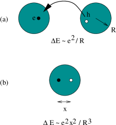
Figure 1: (a) Polarization in the standard AES model involves charge asymmetry between different grains. For weak intergrain tunneling, the energy $\Delta E$ associated with the polarization is of the order of the charging energy of the grain, $e^{2}/R.$ (b) Polarization due to uneven distribution of charge within a grain. Such polarization excitations cost less energy than case (a) but are not considered in the standard AES approach. The filled large circles denote grains, and $e$ and $h$ denote electron excess and deficit, respectively.

I.4 Purpose of this paper and results

In this paper, we generalize the Ambegaokar-Eckern-Schön (AES) model for a regular array of spherical grains to include dipole (polarization) as well as monopole (charge) degrees of freedom. Using this new effective field theory, we are able to calculate the conductivity as a function of temperature as well as of frequency:

1. Using a Kubo formula, we find that the optical conductivity of isolated grains is mainly due to intragrain dipole oscillations,

   $$\sigma(\omega,T) =-\frac{ine^{2}f}{m}\frac{\omega}{\omega^{2}-\omega_{r}^{2}-i|\omega|/\tau_{\text{grain}}},$$

   where $\tau_{\text{grain}}^{-1}$ is the relaxation rate for intragrain scattering and consists of, apart from the classical Drude relaxation in a bulk metal, additional finite-volume effects such as Landau damping.Kawabata and Kubo (1966); Wood and Ashcroft (1982); Kreibig and Genzel (1985)

2. At finite intergrain tunneling, we find that there is a small additional “monopole” contribution $\sigma_{\mathrm{AES}}(\omega,T)$ due to intergrain charge oscillations, and that intergrain tunneling also imparts an extra width $\Gamma$ to the dipole resonance:

   $$\sigma(\omega) \approx\sigma_{\mathrm{AES}}(\omega,T)-\frac{ine^{2}f}{m}\frac{\omega}{\omega^{2}-\omega_{r}^{2}-i|\omega|/\tau_{\text{rel}}},$$

   where $\tau_{\text{rel}}^{-1}=\tau_{\text{grain}}^{-1}+\Gamma(\omega,T).$ At finite temperature, $\sigma_{\mathrm{AES}}(0,T)$ is finite and gives the DC conductivity of the granular array. $\Gamma(\omega,T)$ depends on the intergrain dimensionless conductance, $g,$ and the grain charging $E_{c}.$ It is independent of $\tau_{\text{grain}}^{-1}$, and has a different temperature dependence.

3. The temperature and frequency dependence of the resonance width $\Gamma(\omega,T)$ is different from $\sigma_{\mathrm{AES}}(\omega,T),$ especially when $\omega,T$ are smaller than the effective charging energy of the grains. At large $\omega,T,$ both $\Gamma$ and $\sigma_{\mathrm{AES}}$ become independent of $\omega,T$ and are proportional to the dimensionless intergrain tunneling conductance, $g.$ Fig.2 illustrates the physical difference between the two. The qualitative difference in the manner in which intergrain tunneling affects $\sigma_{\mathrm{AES}}$ and $\Gamma$ cannot be explained by a simple effective medium approximation.Landauer (1952)

4. The optical conductivity of a granular metal is physically different from a dirty insulator with Coulomb interaction even though both show similar features. For both systems, $\sigma(\omega)$ vanishes as a power law at low and high frequencies and has a maximum at intermediate frequencies. However, for a granular metal this maximum is due to resonant polarization oscillations, whereas for a dirty insulator the maximum is just due to a crossover and is not associated with any resonance.

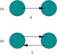
Figure 2: Physically different mechanisms involving intergrain tunneling processes that determine the DC conductivity $\sigma$ (that measures the escape rate of an electron from the grain) and the relaxation rate of polarization oscillations $\Gamma.$ (a) Coulomb blockade of intergrain tunneling, especially at small values of $g,$ suppresses electron escape from the grains leading to $\sigma\sim\exp(-E_{c}/T)$ at low temperatures. (b) A polarization oscillation does not result in a net transfer of charge and therefore no strong Coulomb blockade at low temperatures. High temperatures and strong intergrain tunneling both wash out Coulomb blockade effects, whereby the two processes show the same temperature dependence. Drude theory predicts the same temperature dependence for $\sigma$ and $\Gamma$.

Our theory neglects the interactions between dipole degrees of freedom on different grains. However, at high frequencies (so that the metal dielectric function approaches unity) or for small $f,$ our approximation approaches the Maxwell Garnett result, Eq.(5), when we use the standard relation $\mathop{\mathrm{Re}}\sigma(\omega)=-\frac{|\omega|}{4\pi}\mathop{\mathrm{Im}}\varepsilon_{\mathrm{eff}}(\omega).$ In many experimental situations, such as two-dimensional granular arrays, it is possible to screen out long-range Coulomb interaction within the sample by using a gate electrode, in which case an effective medium treatment is not necessary. In any case, the dipole-dipole interactions can be modeled with a matrix if necessary, just as the monopole-monopole interactions are included in the original AES model as the capacitance matrix. For simplicity, we also ignore possible effects arising from the non-uniformity of the shape of the metallic particles.

I.5 Arrangement of the paper

In Sec.II we introduce our model of granular metals: an array of spherical metallic grains with interacting electrons and a finite intergrain hopping. We then make a multipole expansion of the potential on the grain in terms of spherical harmonics up to the $l=1$ (dipole) component. In Sec.III we develop an effective field theory in terms of the monopole and dipole components of the potential fluctuations: this is a generalization of the AES theory of transport in granular metals. Optical conductivity is calculated in Sec.IV. First we consider isolated grains and calculate the optical conductivity using the Kubo formula approach as well as from the dielectric function. The calculation with the dielectric function is much less tedious. The result agrees with classical expressions for the optical conductivity of isolated grains. Next we consider the case of finite intergrain tunneling and study the differences from the classical optical conductivity. An explicit expression for the broadening of the polarization resonance, $\Gamma,$ is obtained. Its temperature and frequency dependence are found to be different from the conductivity of the granular metal obtained from the AES model. The paper concludes (Sec.V) with a discussion of the results and open problems for further study.

II Model

We consider the following action for the granular metal array,

$$S =\frac{e^{2}}{2}\sum_{\mathbf{ij}}\int_{\tau\mathbf{x_{i}}\mathbf{x}_{j}}\rho(\mathbf{x_{i}},\tau)\rho(\mathbf{x_{j}},\tau)\frac{1}{|\mathbf{x_{i}}-\mathbf{x_{j}}|}+$$

$$+\sum_{\mathbf{i}}\int_{\tau\mathbf{x_{i}}}\psi_{\tau\mathbf{x_{i}}}^{\dagger}[\partial_{\tau}+\xi(-i\nabla_{\mathbf{x}_{\mathbf{i}}})]\psi_{\tau\mathbf{x_{i}}}+$$

$$+\sum_{\langle\mathbf{ij}\rangle}\int_{\tau\mathbf{x_{i}}\mathbf{x}_{\mathbf{j}}}t_{\mathbf{x_{i}},\mathbf{x}_{\mathbf{j}}}\psi_{\tau\mathbf{x_{i}}}^{\dagger}\psi_{\tau\mathbf{x}_{\mathbf{j}}},$$ (10)

where $\rho(\mathbf{x_{i}},\tau)=(\psi_{\tau\mathbf{x_{i}}}^{\dagger}\psi_{\tau\mathbf{x_{i}}\tau}-Q_{0\mathbf{i}})\Theta(|\mathbf{x_{i}}|-R)$ is the excess electronic charge density at position $\mathbf{x_{i}}$ in the $\mathbf{i}^{th}$ grain of radius $R,$ $\xi(-i\nabla_{\mathbf{i}})=\epsilon(-i\nabla_{\mathbf{x}_{\mathbf{i}}})-\mu=\mathbf{p}_{\mathbf{x}_{\mathbf{i}}}^{2}/2m-\mu,$ $\mathbf{a}$ is a lattice translation vector, and $t_{\mathbf{x_{i}},\mathbf{x_{j}}}$ is the intergrain hopping amplitude. Integrals over $\tau$ are understood to go from 0 to $\beta$. We assume the intergrain hopping amplitude has a white-noise distribution,

$$\langle t_{\mathbf{x_{i}},\mathbf{x}_{\mathbf{j}}}t_{\mathbf{x_{k}},\mathbf{x}_{\mathbf{l}}}\rangle =|t|^{2}\delta(\mathbf{x_{i}}-\mathbf{x_{l}})\delta(\mathbf{x_{j}}-\mathbf{x_{k}}).$$ (11)

where angle brackets denote disorder averaging.

Next we decouple the Coulomb interaction in Eq.(10) through a Hubbard-Stratonovich field, $V_{\mathbf{i}}(\mathbf{x_{i}})$, that has the physical meaning of the electrostatic potential. The interaction part of the action is

$$S_{int} =-\frac{1}{2e^{2}}\sum_{\mathbf{ij}}\int_{\tau\mathbf{x_{i}}\mathbf{x_{j}}}\!\!\!\!\!C(\mathbf{x_{i}},\mathbf{x_{j}})V_{\mathbf{i}}(\mathbf{x_{i}},\tau)V_{\mathbf{j}}(\mathbf{x_{j}},\tau)$$

$$+\sum_{\mathbf{i}}\int_{\tau\mathbf{x_{i}}}\psi_{\tau\mathbf{x_{i}}}^{\dagger}V_{\mathbf{i}}(\mathbf{x_{i}},\tau)\psi_{\tau\mathbf{x_{i}}},$$ (12)

where $\int_{\mathbf{x_{j}}}C(\mathbf{x_{i}},\mathbf{x_{j}})\frac{1}{|\mathbf{x_{j}}-\mathbf{x_{k}}|}=\delta(\mathbf{x_{i}}-\mathbf{x_{k}})$ subject to appropriate boundary conditions at the metallic grains; thus $C(\mathbf{x_{i}},\mathbf{x_{j}})$ is proportional to the Laplace operator.

For simplicity, we will consider grains sufficiently far apart so that the mutual interaction of electrons on different grains is small compared to the interaction of electrons within individual grains. With this simplification, the interaction part of the action becomes

$$S_{int} \approx-\frac{1}{8\pi e^{2}}\sum_{\mathbf{i}}\int_{\tau\mathbf{x}}\,\mathbf{E_{i}}(\mathbf{x},\tau)\cdot\mathbf{E_{i}}(\mathbf{x},\tau)+$$

$$+\sum_{\mathbf{i}}\int_{\tau\mathbf{x_{i}}}\psi_{\tau\mathbf{x_{i}}}^{\dagger}V_{\mathbf{i}}(\mathbf{x_{i}},\tau)\psi_{\tau\mathbf{x_{i}}},$$ (13)

$\mathbf{E_{i}}(\mathbf{x},\tau)=-\nabla V_{\mathbf{i}}(\mathbf{x},\tau)$ is the electric field at $\mathbf{x}$ due to charge on an isolated grain at $\mathbf{i}.$ The potential away from the boundary may be expanded in a basis of eigenfunctions of the Laplace equation,

$$V_{\mathbf{i}}(\mathbf{x},\tau) =\sum_{lm}A_{\mathbf{i}}^{lm}(\tau)\left(\frac{r}{R}\right)^{l}Y_{lm}(\theta,\phi)\,\,\,\,(r<R),$$

$$V_{\mathbf{i}}(\mathbf{x},\tau) =\sum_{lm}B_{\mathbf{i}}^{lm}(\tau)\left(\frac{R}{r}\right)^{l+1}Y_{lm}(\theta,\phi)\,\,\,\,(r>R),$$

where $r=|\mathbf{x}|$. Continuity of $V_{\mathbf{i}}(\mathbf{x},\tau)$ at the boundary requires that $A_{\mathbf{i}}^{lm}(\tau)=B_{\mathbf{i}}^{lm}(\tau).$ For the purposes of this paper, it is sufficient to retain just the monopole component (average potential)

$$V_{\mathbf{i}}(l=0;\mathbf{x},\tau) =\left\{\begin{array}[]{r}V_{\mathbf{i}0}(\tau),\qquad r<R\\ V_{\mathbf{i}0}(\tau)(R/r),\qquad r>R,\end{array}\right.$$

and the dipole components (electric field),

$$V_{\mathbf{i}}^{(\alpha)}(l=1;\mathbf{x},\tau) =\left\{\begin{array}[]{r}V_{\mathbf{i}1}^{(\alpha)}(\tau)(x^{\alpha}/R),\qquad r<R\\ V_{\mathbf{i}1}^{(\alpha)}(\tau)(R^{2}x^{\alpha}/r^{3}),\qquad r>R.\end{array}\right.$$

Using the definition $\mathbf{E_{i}}(\mathbf{x},\tau)=-\nabla V_{\mathbf{i}}(\mathbf{x},\tau)$ the interaction part of the action, Eq.(13) takes the form

$$S_{int}\approx -\frac{R}{2e^{2}}\sum_{\mathbf{i}}\int_{\tau}\left[(V_{\mathbf{i}0}(\tau))^{2}+\sum_{\alpha}(V_{\mathbf{i}1}^{(\alpha)}(\tau))^{2}\right]$$

$$+ \sum_{\mathbf{i}}\int_{\tau\mathbf{x_{i}}}\!\!\!\psi_{\tau\mathbf{x_{i}}}^{\dagger}\left[V_{\mathbf{i}0}+\sum_{\alpha}V_{\mathbf{i}1}^{(\alpha)}(x_{\mathbf{i}}^{\alpha}/R)\right]\psi_{\tau\mathbf{x_{i}}}.$$ (14)

Now make the gauge transformations

$$\psi_{\tau\mathbf{x_{i}}}\rightarrow\psi_{\tau\mathbf{x_{i}}}\,e^{-i\varphi_{\mathbf{i}0}(\tau)-i\sum_{\alpha}\varphi_{\mathbf{i}1}^{(\alpha)}(\tau)(x_{\mathbf{i}}^{\alpha}/R)},$$ (15)

$$V_{\mathbf{i}0}(\tau)=i\partial_{\tau}\varphi_{\mathbf{i}0},\,\,V_{\mathbf{i}1}^{(\alpha)}(\tau)=i\partial_{\tau}\varphi_{\mathbf{i}1}^{(\alpha)}.$$ (16)

to eliminate $V_{\mathbf{i}0}(\tau)$ and replace $V_{\mathbf{i}1}(\tau)$ by a time-dependent vector potential,

$$S_{el} =\sum_{\mathbf{i}}\int_{\tau\mathbf{x_{i}}}\psi_{\tau\mathbf{x}_{\mathbf{i}}}^{\dagger}\bigg{[}\partial_{\tau}+\xi(-i\nabla_{\mathbf{x}_{\mathbf{i}}})+V_{\mathbf{i}0}+$$

$$+\sum_{\alpha}V_{\mathbf{i}1}^{(\alpha)}(x_{\mathbf{i}}^{\alpha}/R)\bigg{]}\psi_{\tau\mathbf{x_{i}}}$$

$$\rightarrow\sum_{\mathbf{i}}\!\!\int_{\tau\mathbf{x_{i}}}\!\!\!\!\psi_{\tau\mathbf{x_{i}}}^{\dagger}\left[\partial_{\tau}+\xi(-i\nabla_{\mathbf{x}_{\mathbf{i}}}-\boldsymbol{\varphi}_{\mathbf{i}1}/R)\right]\psi_{\tau\mathbf{x_{i}}}.$$ (17)

The gauge transformations also dress the tunneling element in Eq.(10) with monopole ($l=0$) and dipole ($l=1$) phase fluctuations,

$$t_{\mathbf{x_{i}},\mathbf{x}_{\mathbf{j}}}\rightarrow\tilde{t}_{\mathbf{x_{i}},\mathbf{x}_{\mathbf{j}}}(\tau)=t_{\mathbf{x_{i}},\mathbf{x}_{\mathbf{j}}}e^{i(\varphi_{\mathbf{i}0}(\tau)-\varphi_{\mathbf{j}0}(\tau))}\times$$

$$\times\exp\left[(i/R)\sum_{\alpha}\left(\varphi_{\mathbf{i}1}^{(\alpha)}(\tau)x_{\mathbf{i}}^{\alpha}-\varphi_{\mathbf{j}1}^{(\alpha)}(\tau)x_{\mathbf{j}}^{\alpha}\right)\right].$$ (18)

III Effective field theory

Integrating out the conduction electrons results in an effective action for the $l=0$ and $l=1$ phase fluctuations:

$$S_{\mathrm{eff}}[\varphi] =\frac{R}{2e^{2}}\sum_{\mathbf{i}}\int_{\tau}\left[\left(\partial_{\tau}\varphi_{\mathbf{i}0}\right)^{2}+\left|\partial_{\tau}\boldsymbol{\varphi}_{\mathbf{i}1}\right|^{2}\right]$$

$$- \text{tr ln}\left[G_{\boldsymbol{\varphi}_{\mathbf{i}1}}^{-1}\delta_{\mathbf{ij}}-\left(\tilde{t}_{\mathbf{x_{i}},\mathbf{x_{j}}}\delta_{\mathbf{j},\mathbf{i}+\mathbf{a}}+\mathbf{i}\leftrightarrow\mathbf{i}+\mathbf{a}\right)\right],$$ (19)

where

$$-G_{\boldsymbol{\varphi}_{\mathbf{i}1}}^{-1} =\partial_{\tau}+\frac{1}{2m}\left(\mathbf{p}_{\mathbf{x}_{\mathbf{i}}}-\frac{\boldsymbol{\varphi}_{\mathbf{i}1}}{R}\right)^{2}-\mu$$ (20)

is the inverse of the electron Green function on grain $\mathbf{i}$ in the absence of intergrain tunneling, and $\tilde{t}_{\mathbf{x}_{\mathbf{i}},\mathbf{x}_{\mathbf{j}}}$ is the dressed tunneling amplitude defined in Eq.(18) and the bare tunneling $t_{\mathbf{x}_{\mathbf{i}},\mathbf{x}_{\mathbf{j}}}$ has a gaussian distribution as in Eq.(11). We study first the effective field theory for isolated grains and then consider the effect of finite intergrain tunneling.

III.1 Isolated grains

In the absence of tunneling, the “bare” effective action $S_{\mathrm{eff}}^{(0)}[\varphi]$ is obtained by expanding the determinant in Eq.(19) up to second order in $\boldsymbol{\varphi}_{\mathbf{i}1}(\tau)$,

$$S_{\mathrm{eff}}^{(0)}[\varphi] =\frac{R}{2e^{2}}\sum_{\mathbf{i}}\int_{\tau}\left[\left(\partial_{\tau}\varphi_{\mathbf{i}0}\right)^{2}+\left|\partial_{\tau}\boldsymbol{\varphi}_{\mathbf{i}1}\right|^{2}\right]$$

$$+\frac{1}{2mR^{2}}\sum_{\mathbf{i}}\left[\int_{\tau\mathbf{x_{I}}}G_{\mathbf{i}}^{(0)}(\mathbf{x_{i}},\mathbf{x_{i}};\tau,\tau)\boldsymbol{\varphi}_{\mathbf{i}1}^{2}(\tau)\right.$$

$$+\frac{1}{m}\int_{\tau\tau^{\prime}\mathbf{x_{i}x_{i}}^{\prime}}\boldsymbol{\varphi}_{\mathbf{i}1}(\tau)\cdot\mathbf{p}_{\mathbf{x}_{\mathbf{i}}}\,G_{\mathbf{i}}^{(0)}(\mathbf{x_{i}},\mathbf{x}^{\prime}_{\mathbf{i}};\tau,\tau^{\prime})$$

$$\times\boldsymbol{\varphi}_{\mathbf{i}1}(\tau^{\prime})\cdot\mathbf{p}_{\mathbf{x}_{\mathbf{i}}^{\prime}}\,G_{\mathbf{i}}^{(0)}(\mathbf{x}^{\prime}_{\mathbf{i}},\mathbf{x_{i}};\tau^{\prime},\tau)\bigg{]},$$ (21)

where $G_{\mathbf{i}}^{(0)}=-\left[\partial_{\tau}+\frac{1}{2m}\mathbf{p}_{\mathbf{x}_{\mathbf{i}}}^{2}-\mu\right]^{-1}$ is the bare electron Green function,

$$G_{\mathbf{i}}^{(0)}(\mathbf{x}_{\mathbf{i}},\mathbf{x}_{\mathbf{i}}^{\prime};\tau,\tau^{\prime}) =T\sum_{\lambda,n}\frac{\psi_{\lambda}(\mathbf{x}_{\mathbf{i}}^{\prime})\psi_{\lambda}^{*}(\mathbf{x}_{\mathbf{i}})}{i\nu_{n}-\xi_{\mathbf{i}\lambda}}e^{-i\nu_{n}(\tau-\tau^{\prime})}$$

$$=\sum_{\lambda}G_{\mathbf{i}\lambda}^{(0)}(\tau,\tau^{\prime})\psi_{\lambda}(\mathbf{x}_{\mathbf{i}}^{\prime})\psi_{\lambda}^{*}(\mathbf{x}_{\mathbf{i}}).$$ (22)

Note that

$$\sum_{\lambda}G_{\mathbf{i}\lambda}^{(0)}(\tau,\tau^{\prime}) \approx\nu(\epsilon_{F})T\sum_{n}\int_{-\tau_{c}^{-1}}^{\tau_{c}^{-1}}d\xi_{\mathbf{i}}\frac{e^{-i\nu_{n}(\tau-\tau^{\prime})}}{i\nu_{n}-\xi_{\mathbf{i}}}$$

$$=-2i\nu(\epsilon_{F})T\sum_{n}e^{-i\nu_{n}(\tau-\tau^{\prime})}\cot^{-1}\nu_{n}\tau_{c}$$ (23)

where $\tau_{c}\sim\epsilon_{F}^{-1}$ is a short time cutoff. For $|\tau-\tau^{\prime}|\gg\tau_{c},$ this simplifies to

$$\sum_{\lambda}G_{\mathbf{i}\lambda}^{(0)}(\tau,\tau^{\prime}) \approx\frac{\pi T\nu(\epsilon_{F})}{\sin\pi T(\tau-\tau^{\prime})}.$$ (24)

We shall use this expression unless stated otherwise.

Eq.(21) can be presented in a more recognizable form as

$$S_{\mathrm{eff}}^{(0)}[\varphi] =\frac{R}{2e^{2}}\sum_{\mathbf{i}}\int_{\tau}\left[\left(\partial_{\tau}\varphi_{\mathbf{i}0}\right)^{2}+\left|\partial_{\tau}\boldsymbol{\varphi}_{\mathbf{i}1}\right|^{2}\right]$$

$$+ \frac{4\pi}{3}\frac{R}{2e^{2}}\sum_{\mathbf{i}\alpha\beta}\int_{\tau,\tau^{\prime}}K_{\mathbf{i}}^{\alpha\beta}(\tau-\tau^{\prime})\varphi_{\mathbf{i}1}^{(\alpha)}(\tau)\varphi_{\mathbf{i}1}^{(\beta)}(\tau^{\prime}).$$ (25)

in terms of the bare electromagnetic response function of the $\mathbf{i}^{th}$ grain,

$$K_{\mathbf{i}}^{\alpha\beta}(\tau-\tau^{\prime})=\delta^{\alpha\beta}\frac{e^{2}}{Vm}\int_{\mathbf{x_{i}}}G_{\mathbf{i}}^{(0)}(\mathbf{x_{i}},\mathbf{x_{i}};\tau,\tau^{\prime})\delta(\tau-\tau^{\prime})+$$

$$\!\!\!\!\!\!+\frac{e^{2}}{Vm^{2}}\int_{\mathbf{x_{i}x}^{\prime}_{\mathbf{i}}}\!\!\!\!\!\!p_{\mathbf{x}_{\mathbf{i}}}^{\alpha}G_{\mathbf{i}}^{(0)}(\mathbf{x_{i}},\mathbf{x}^{\prime}_{\mathbf{i}};\tau,\tau^{\prime})p_{\mathbf{x}_{\mathbf{i}}^{\prime}}^{\beta}G_{\mathbf{i}}^{(0)}(\mathbf{x}^{\prime}_{\mathbf{i}},\mathbf{x_{i}};\tau^{\prime},\tau),\,\,\,\,$$ (26)

where $V=(4\pi/3)R^{3}$ is the volume of the grain. In a bulk metal, the two terms in the electromagnetic response function in Eq.(26) would correspond to the diamagnetic and paramagnetic parts of the bulk conductivity $\sigma(\omega)=K(\omega)/i\omega$. In a finite system, the situation is trickier. The frequency dependence of $K$ is

$$K_{\mathbf{i}}^{\alpha\beta}(i\omega_{m})=\delta^{\alpha\beta}\frac{ne^{2}}{m}\left[1+\frac{2}{mN}\sum_{\lambda\lambda^{\prime}}\frac{f(\xi_{\mathbf{i}\lambda})\xi_{\mathbf{i},\lambda\lambda^{\prime}}|p_{\mathbf{i},\lambda\lambda^{\prime}}^{\alpha}|^{2}}{\omega_{m}^{2}+\xi_{\mathbf{i},\lambda\lambda^{\prime}}^{2}}\right],$$ (27)

where $\lambda,\lambda^{\prime}$ label the eigenvalues of the free electron Hamiltonian of a grain, $\xi_{\mathbf{i},\lambda\lambda^{\prime}}=\xi_{\mathbf{i}\lambda}-\xi_{\mathbf{i}\lambda^{\prime}},$ $f(\xi)=[e^{\beta\xi}+1]^{-1}$ is the Fermi-Dirac distribution function, and $p_{\mathbf{i},\lambda\lambda^{\prime}}^{\alpha}=\langle\lambda|p_{\mathbf{i}}^{\alpha}|\lambda^{\prime}\rangle.$ $n=N/V$ is the number density of electrons in a grain. If the temperature (or frequency) is much smaller than the level separation $\delta=\xi_{\lambda\lambda^{\prime}}^{avg}\sim\epsilon_{F}/N,$ we expand the right hand side of Eq.(27) in ascending powers of $\omega_{m}:$

$$K_{\mathbf{i}}^{\alpha\beta}(i\omega_{m})\approx\delta^{\alpha\beta}\frac{ne^{2}}{m}\bigg{[}1+\frac{2}{mN}\sum_{\lambda\lambda^{\prime}}\frac{f(\xi_{\mathbf{i}\lambda})|p_{\mathbf{i},\lambda\lambda^{\prime}}^{\alpha}|^{2}}{\xi_{\mathbf{i},\lambda\lambda^{\prime}}}$$

$$-\frac{2}{mN}\omega_{m}^{2}\sum_{\lambda\lambda^{\prime}}\frac{f(\xi_{\mathbf{i}\lambda})|p_{\mathbf{i},\lambda\lambda^{\prime}}^{\alpha}|^{2}}{\xi_{\mathbf{i},\lambda\lambda^{\prime}}^{3}}\bigg{]}+O(\omega_{m}^{4}).$$ (28)

The static part of Eq.(28) can be shown to vanish using the Reiche-Thomas-Kuhn sum rule,Reiche and Thomas (1925); Kuhn (1925)

$$\frac{2}{m}\sum_{\lambda^{\prime}}\frac{|p_{\mathbf{i},\lambda\lambda^{\prime}}^{\alpha}|^{2}}{\xi_{\mathbf{i},\lambda\lambda^{\prime}}} =-1,$$ (29)

along with the identity $\sum_{\lambda}f(\xi_{\mathbf{i}\lambda})=N.$ Combining Eq.(25) and Eq.(28), one finds that the surviving contribution in Eq.(28) makes a finite size quantum correction to the RPA dielectric constantGorkov and Eliashberg (1965); Strässler et al. (1972); Cohen et al. (1973); Wood and Ashcroft (1982); Kreibig and Vollmer (1995); Henning et al. (1999), $\varepsilon^{RPA}=1-\frac{2e^{2}}{m^{2}R^{3}}\sum_{\lambda\lambda^{\prime}}\frac{f(\xi_{\mathbf{i}\lambda})|p_{\mathbf{i},\lambda\lambda^{\prime}}^{\alpha}|^{2}}{\xi_{\mathbf{i},\lambda\lambda^{\prime}}^{3}}\sim 1-(k_{F}a_{0})(R/a_{0})^{2},$ where $a_{0}$ is a small length of the order of a lattice constant. As a result, even for metallic grains a few tens of lattice constants across, the static dielectric constant rapidly approaches bulk values (where is it infinity), and the polarizability, $\alpha=R^{3}(\varepsilon^{RPA}-1)/(\varepsilon^{RPA}+2),$ approaches the classical value, $\alpha_{\text{classical}}=R^{3}.$

The sum rule enables us to recast the electromagnetic response function as

$$K_{\mathbf{i}}^{\alpha\beta}(i\omega_{m}) =-\delta^{\alpha\beta}\frac{2e^{2}}{Vm^{2}}\omega_{m}^{2}\!\sum_{\lambda\lambda^{\prime}}\frac{f(\xi_{\mathbf{i}\lambda})|p_{\mathbf{i},\lambda\lambda^{\prime}}^{\alpha}|^{2}}{\xi_{\mathbf{i},\lambda\lambda^{\prime}}(\omega_{m}^{2}+\xi_{\mathbf{i},\lambda\lambda^{\prime}}^{2})},$$ (30)

which is a known result. For the rest of the paper, unless stated otherwise, we shall assume that the temperature (or frequency) is much larger than the level separation $(T/\delta\gg 1)$. Then, using Eq.(29) and Eq.(30), we obtain

$$K_{\mathbf{i}}^{\alpha\beta}(i\omega_{m}) \approx\delta^{\alpha\beta}\frac{ne^{2}}{m},\qquad T/\delta\gg 1,$$ (31)

that is, the value for the clean bulk metal; this is the diamagnetic response due to electron acceleration in an electric field. Hence, Eq.(25) becomes

$$S_{\mathrm{eff}}^{(0)}[\varphi] =\frac{R}{2e^{2}}\sum_{\mathbf{i}}\int_{\tau}\left[\left(\partial_{\tau}\varphi_{\mathbf{i}0}\right)^{2}+\left|\partial_{\tau}\boldsymbol{\varphi}_{\mathbf{i}1}\right|^{2}+\omega_{r}^{2}\left|\boldsymbol{\varphi}_{\mathbf{i}1}\right|^{2}\right]$$ (32)

where $\omega_{r}$ is the resonance frequency for a metallic sphere,

$$\omega_{r}^{2} =\frac{4\pi}{3}\frac{ne^{2}}{m},$$ (33)

we introduced in Eq.(8). In a collisionless bulk metal, the paramagnetic part of the electromagnetic response function defined in Eq.(26) vanishes. However, in a finite-size grain, if one can treat the quasiparticle excitations in the grain as a continuum (this is so if the temperature is not too low, $T\gg\delta$), the paramagnetic part is finite and gives rise to a finite relaxation of the oscillations through disintegration into incoherent particle-hole excitations.Kawabata and Kubo (1966); Wood and Ashcroft (1982) The relaxation time has been shown in numerous worksKawabata and Kubo (1966); Wood and Ashcroft (1982); Kreibig and Genzel (1985) to be of the order of the time of flight, $R/v_{F}.$ Physically, the relaxation is due to Landau damping of plasma oscillations at a finite wavevector: the minimum wavevector in a grain of size $R$ is of the order of $\pi/R.$ Other inelastic processes such as phonon scattering will also contribute to relaxation.

III.2 Finite intergrain tunneling

We now obtain the effective field theory when intergrain tunneling is finite. At not too low temperatures,Beloborodov et al. (2001); Efetov and Tschersich (2002) $T\gg\text{max }(|t|^{2}\delta,\delta),$ and for large enoughZárand et al. (2000) grains $(k_{F}R)^{2}\gg 1,$ it suffices to expand the electron determinant in Eq.(19) up to $O(t^{2})$,

$$S_{\mathrm{eff}}^{\mathrm{tun}}[\varphi]=\frac{1}{2}\sum_{\mathbf{i},\mathbf{a}}\int_{\tau\tau^{\prime}\mathbf{x_{i}}\mathbf{x}_{\mathbf{i}}^{\prime}\mathbf{x}_{\mathbf{i}+\mathbf{a}}\mathbf{x}_{\mathbf{i}+\mathbf{a}}^{\prime}}\!\!\!\!\tilde{t}_{\mathbf{x}_{\mathbf{i}}^{\prime},\mathbf{x}_{\mathbf{i}+\mathbf{a}}^{\prime}}(\tau^{\prime})\tilde{t}_{\mathbf{x_{\mathbf{i}+\mathbf{a}}},\mathbf{x_{i}}}(\tau)$$

$$\times G_{\boldsymbol{\varphi}_{\mathbf{i}1}}(\mathbf{x}_{\mathbf{i}},\mathbf{x}^{\prime}_{\mathbf{i}};\tau,\tau^{\prime})G_{\boldsymbol{\varphi}_{\mathbf{i}+\mathbf{a},1}}(\mathbf{x}^{\prime}_{\mathbf{i}+\mathbf{a}},\mathbf{x}_{\mathbf{\mathbf{i}+\mathbf{a}}};\tau^{\prime},\tau)$$

$$=\frac{|t|^{2}}{2}\sum_{\mathbf{i},\mathbf{a}}\int_{\tau\tau^{\prime}\mathbf{x_{i}}\mathbf{x}_{\mathbf{i}+\mathbf{a}}}G(\mathbf{x}_{\mathbf{i}},\mathbf{x}{}_{\mathbf{i}};\tau,\tau^{\prime})G_{\boldsymbol{\varphi}_{\mathbf{i}+\mathbf{a},1}}(\mathbf{x}{}_{\mathbf{i}+\mathbf{a}},\mathbf{x}_{\mathbf{\mathbf{i}+\mathbf{a}}};\tau^{\prime},\tau)$$

$$e^{i(\varphi_{\mathbf{ij},0}(\tau^{\prime})-\varphi_{\mathbf{ij},0}(\tau))}$$

$$e^{i(1/R)(\boldsymbol{\varphi}_{\mathbf{i}1}(\tau^{\prime})-\boldsymbol{\varphi}_{\mathbf{i}1}(\tau))\cdot\mathbf{x_{i}}}e^{-i(1/R)(\boldsymbol{\varphi}_{\mathbf{j}1}(\tau^{\prime})-\boldsymbol{\varphi}_{\mathbf{j}1}(\tau))\cdot\mathbf{x}_{\mathbf{j}}},$$ (34)

where $\varphi_{\mathbf{ij},0}(\tau)=\varphi_{\mathbf{i}0}(\tau)-\varphi_{\mathbf{j}0}(\tau).$ The $\boldsymbol{\varphi}_{\mathbf{i}1}$ dependence in Eq.(34) comes from the exponential as well as from the the Green functions, $G_{\boldsymbol{\varphi}_{\mathbf{i}1}}(\mathbf{x}_{\mathbf{i}},\mathbf{x}_{\mathbf{i}};\tau,\tau^{\prime}),$ etc. We show in Appendix B that the contribution arising from the expansion of $G_{\boldsymbol{\varphi}_{\mathbf{i}1}}(\mathbf{x}_{\mathbf{i}},\mathbf{x}_{\mathbf{i}};\tau,\tau^{\prime})$ etc. in powers of $\boldsymbol{\varphi}_{\mathbf{i}1}$ is insignificant compared to that coming from the exponential. Therefore we expand only the exponential in Eq.(34) up to second order in $\boldsymbol{\varphi}_{\mathbf{i}1}$ etc. and ignore the $\boldsymbol{\varphi}_{\mathbf{i}1}$ dependence of the Green functions. Thus the tunneling part of the effective action is

$$S_{\mathrm{eff}}^{\mathrm{tun}}[\varphi] \approx\!\!|t|^{2}\!\!\sum_{\mathbf{i},\mathbf{a};\lambda\lambda^{\prime}}\!\int_{\tau\tau^{\prime}}\!\!\!\!\Pi_{\mathbf{i},\mathbf{i}+\mathbf{a}}(\tau,\tau^{\prime})G_{\mathbf{i}\lambda}^{(0)}(\tau,\tau^{\prime})G_{\mathbf{i}+\mathbf{a},\lambda^{\prime}}^{(0)}(\tau^{\prime},\tau)$$

$$- \frac{|t|^{2}}{6R^{2}}\!\!\sum_{\mathbf{i},\mathbf{a};\lambda\lambda^{\prime}}\int_{\tau\tau^{\prime}}\!\!\!\!\!\!\Pi_{\mathbf{i},\mathbf{i}+\mathbf{a}}(\tau,\tau^{\prime})G_{\mathbf{i}\lambda}^{(0)}(\tau,\tau^{\prime})G_{\mathbf{i}+\mathbf{a},\lambda^{\prime}}^{(0)}(\tau^{\prime},\tau)$$

$$\times \big{[}r_{\mathbf{i}\lambda}^{2}(\boldsymbol{\varphi}_{\mathbf{i}1}(\tau^{\prime})-\boldsymbol{\varphi}_{\mathbf{i}1}(\tau))^{2}$$

$$+r_{\mathbf{i}+\mathbf{a},\lambda^{\prime}}^{2}(\boldsymbol{\varphi}_{\mathbf{i}+\mathbf{a},1}(\tau^{\prime})-\boldsymbol{\varphi}_{\mathbf{i}+\mathbf{a},1}(\tau))^{2}\big{]}$$ (35)

where

$$\Pi_{\mathbf{i},\mathbf{i}+\mathbf{a}}(\tau,\tau^{\prime}) =\cos(\varphi_{\mathbf{i},\mathbf{i}+\mathbf{a},0}(\tau)\!-\!\varphi_{\mathbf{i},\mathbf{i}+\mathbf{a},0}(\tau^{\prime}))$$ (36)

and $r_{\mathbf{i}\lambda}^{2}=\langle\mathbf{i}\lambda|\hat{r}^{2}|\mathbf{i}\lambda\rangle$ are the matrix elements of $\hat{r}^{2}=|\mathbf{\hat{\mathbf{x}}}|^{2}$ with the eigenstates of grain $\mathbf{i}$. For a spherical grain, the eigenfunctions are spherical Bessel functions $j_{n}(\kappa_{nl}r/R)Y_{lm}(\theta,\phi),$ where $\kappa_{nl}$ is the $l^{th}$ zero of $j_{n}(x).$ Numerically evaluating the matrix elements we find they range between $0.28R^{2}$ and $R^{2}.$ In particular, $\lim_{n\rightarrow\infty}(r^{2})_{n1}=R^{2},$ and $\lim_{l\rightarrow\infty}(r^{2})_{nl}=R^{2}/3.$ Thus the matrix elements of $r^{2}$ do not vary strongly and are of the order of $R^{2}.$ Hence Eq.(35) may be written

$$S_{\mathrm{eff}}^{\mathrm{tun}}[\varphi]\approx-\frac{\pi gT^{2}}{2}\sum_{\mathbf{i},\mathbf{a}}\int_{\tau\tau^{\prime}}\frac{\Pi_{\mathbf{i},\mathbf{i}+\mathbf{a}}(\tau,\tau^{\prime})}{\sin^{2}\pi T(\tau-\tau^{\prime})}$$

$$+\frac{\pi gT^{2}b}{2}\sum_{\mathbf{i},\mathbf{a}}\int_{\tau\tau^{\prime}}\frac{\Pi_{\mathbf{i},\mathbf{i}+\mathbf{a}}(\tau,\tau^{\prime})}{\sin^{2}\pi T(\tau-\tau^{\prime})}$$

$$\times\big{[}(\boldsymbol{\varphi}_{\mathbf{i}1}(\tau^{\prime})-\boldsymbol{\varphi}_{\mathbf{i}1}(\tau))^{2}+(\boldsymbol{\varphi}_{\mathbf{i}+\mathbf{a},1}(\tau^{\prime})-\boldsymbol{\varphi}_{\mathbf{i}+\mathbf{a},1}(\tau))^{2}\big{]};\qquad$$ (37)

here $b\sim 0.1$ is a constant, $g$ is the dimensionless intergrain tunneling conductance

$$g =2\pi|t|^{2}\nu(\epsilon_{F})^{2},$$ (38)

Eqs.(32) and (37) form the effective action, $S_{\mathrm{eff}}[\varphi]=S_{\mathrm{eff}}^{(0)}[\varphi]+S_{\mathrm{eff}}^{\mathrm{tun}}[\varphi]$, which generalizes the AES action to include the physics of dipolar oscillations. This may be presented as $S_{\mathrm{eff}}[\varphi]\approx S_{\mathrm{AES}}[\varphi_{0}]+S_{pol}[\varphi_{0}]$ where

$$S_{\mathrm{pol}}[\varphi]\approx$$

$$\frac{T}{2(e^{2}/R)}\sum_{\mathbf{i},m}(\omega_{m}^{2}+\omega_{r}^{2})\boldsymbol{\varphi}_{\mathbf{i}1}(\omega_{m})\cdot\boldsymbol{\varphi}_{\mathbf{i}1}(-\omega_{m})+$$

$$\frac{T}{4(e^{2}/R)}\sum_{\mathbf{i}\mathbf{a}}\Gamma_{\mathbf{i},\mathbf{i}+\mathbf{a}}(i\omega_{m})|\omega_{m}|\times$$

$$[\boldsymbol{\varphi}_{\mathbf{i}1}(\omega_{m})\cdot\boldsymbol{\varphi}_{\mathbf{i}1}(-\omega_{m})+\boldsymbol{\varphi}_{\mathbf{i}+\mathbf{a},1}(\omega_{m})\cdot\boldsymbol{\varphi}_{\mathbf{i}+\mathbf{a},1}(-\omega_{m})],$$ (39)

where

$$S_{\mathrm{AES}}[\varphi_{0}] =\frac{1}{2(e^{2}/R)}\sum_{\mathbf{i}}\int_{\tau}(\partial_{\tau}\varphi_{\mathbf{i}0})^{2}+$$

$$-\frac{\pi gT^{2}}{2}\sum_{\mathbf{ia}}\int_{\tau\tau^{\prime}}\frac{\Pi_{\mathbf{i},\mathbf{i}+\mathbf{a}}(\tau,\tau^{\prime})}{\sin^{2}\pi T(\tau-\tau^{\prime})}\qquad$$ (40)

is the standard Ambegaokar-Eckern-Schön (AES) model for normal granular metals and

$$\Gamma_{\mathbf{i},\mathbf{i}+\mathbf{a}}(i\omega_{m})=\frac{e^{2}4\pi gbT^{2}}{R|\omega_{m}|}\!\!\int_{\tau}(1-e^{i\omega_{m}\tau})\frac{\Pi_{\mathbf{i},\mathbf{i}+\mathbf{a}}(\tau,0)}{\sin^{2}(\pi T\tau)}.$$ (41)

The quantities $\Pi$ and $\Gamma$ are functionals of $\varphi_{0}$. In principle, fluctuations of $\varphi_{0}$ and of $\varphi_{1}$ can influence each other since they both appear in $S\mathrm{{}_{\mathrm{pol}}}$. In practice, it is sufficient to calculate the correlator $\langle\Pi[\varphi_{0}]\rangle$ for $S\mathrm{{}_{\mathrm{\mathrm{AES}}}}$ alone, and to use this mean value in $S\mathrm{{}_{\mathrm{pol}}}$ to determine the fluctuations of $\varphi_{1}$. To justify this, we show that fluctuations of $\varphi_{1}$ have a negligible effect on the “kernel” for $\varphi_{0}$ . If in Eq.(37) we average over the fields $\boldsymbol{\varphi}_{\mathbf{i}1}$ using their bare propagator in the absence of tunneling (see Eq.(32)),

$$\langle(\boldsymbol{\varphi}_{\mathbf{i}1}(\tau)-\boldsymbol{\varphi}_{\mathbf{i}1}(0))^{2}\rangle =3(e^{2}/R)T\sum_{n}\frac{(1-e^{-i\omega_{n}\tau})}{\omega_{n}^{2}+\omega_{r}^{2}}$$

$$=3\frac{e^{2}/R}{2\omega_{r}}\coth(\omega_{r}/2T)(1-e^{-\omega_{r}|\tau|}).$$ (42)

Thus at long times, $\omega_{r}|\tau|\gg 1,$ the correction to the tunneling term of the AES model due to dipole modes is smaller than the bare value by a factor of $(e^{2}/R)/\omega_{r}.$ In most common cases of granular metals, this ratio is of the order of $10^{-2},$ as $E_{c}\sim 10^{2}K$ and $\omega_{r}\sim 10^{4}K.$ At short times, $\omega_{r}|\tau|\ll 1,$ the correction is smaller than the bare value by a factor $\omega_{r}|\tau|\ll 1.$ Thus under most common physical circumstances, our approximation is valid.

For finite tunneling, the propagator for the dipole modes is that of a damped harmonic oscillator,

$${\mathcal{D}}_{\mathbf{ij}}^{\alpha\beta}(i\omega_{n})=\frac{\delta^{\alpha\beta}\delta_{\mathbf{i}\mathbf{j}}(e^{2}/R)}{\omega_{n}^{2}+\omega_{r}^{2}+\Gamma(\omega_{n})|\omega_{n}|},$$ (43)

where the resonance linewidth is

$$\Gamma =\sum_{\mathbf{a}}\Gamma_{\mathbf{i},\mathbf{i}+\mathbf{a}}.$$ (44)

IV Optical conductivity

In this section we calculate the optical conductivity of isolated metallic grains and then generalize it to finite intergrain tunneling. For isolated grains, we show that the optical conductivity may be obtained in two ways: directly from the Kubo formula, and from the dielectric function.

IV.1 Isolated grains

IV.1.1 Kubo formula approach

We first calculate the optical conductivity for isolated grains using the Kubo formula approach. For this we introduce an infinitesimal vector potential $\mathbf{A}_{\tau\mathbf{x}}$ that couples to the current $\mathbf{j}_{\mathbf{\tau\mathbf{x}}}$ and is related to the electric field through $\mathbf{E}_{\tau\mathbf{x}}=i\partial_{\tau}\mathbf{A}_{\tau\mathbf{x}}.$ The electronic kinetic energy becomes

$$\epsilon(\tilde{\mathbf{p}}_{\tau\mathbf{x}_{\mathbf{i}}}) \rightarrow\epsilon(\tilde{\mathbf{p}}_{\mathbf{x}_{\mathbf{i}}}-\tfrac{e}{c}\mathbf{A}_{\tau\mathbf{x}_{\mathbf{i}}})$$

$$=\epsilon(\tilde{\mathbf{p}}_{\mathbf{x}_{\mathbf{i}}})-\tfrac{e}{mc}\mathbf{A}_{\tau\mathbf{x}_{\mathbf{i}}}\cdot\tilde{\mathbf{p}}_{\mathbf{x}_{\mathbf{i}}}+\tfrac{e^{2}}{2mc^{2}}\mathbf{A}_{\tau\mathbf{x}_{\mathbf{i}}}^{2},$$ (45)

where $\mathbf{p}_{\mathbf{x}_{\mathbf{i}}}=-i\boldsymbol{\nabla}_{\mathbf{x}_{\mathbf{i}}}$ and $\tilde{\mathbf{p}}_{\tau\mathbf{x}_{\mathbf{i}}}=\mathbf{p}_{\mathbf{x}_{\mathbf{i}}}-\frac{1}{R}\boldsymbol{\varphi}_{\mathbf{i}1}(\tau)$, and we have chosen the gauge $\nabla\cdot\mathbf{A}=0.$ The optical conductivity tensor $\sigma^{\alpha\beta}$ is the coefficient relating the $\mathbf{q}=0$ component of the current,

$$j_{\tau}^{\alpha}[\mathbf{A};\mathbf{q}] =-\frac{c}{Z_{0}}\int d\mathbf{x}\,e^{-i\mathbf{q}\cdot\mathbf{x}}\int D(\text{fields})\frac{\delta S[\mathbf{A}]}{\delta A_{\tau\mathbf{x}}^{\alpha}}e^{-S[\mathbf{A}]},$$ (46)

to the $\mathbf{q}=0$ component of the electric field $E_{\tau\mathbf{x}}^{\beta}=i\partial_{\tau}A_{\tau\mathbf{x}}^{\beta},$

$$\sigma^{\alpha\beta}(\tau,\tau^{\prime}) =Tc^{2}\sum_{m}\sigma^{\alpha\beta}(i\omega_{m})e^{-i\omega_{m}(\tau^{\prime}-\tau)}$$

$$=\frac{\delta j_{\tau}^{\alpha}[\mathbf{A};\mathbf{q}=0]}{\delta E_{\tau^{\prime}}^{\beta}(\mathbf{q}=0)}\bigg{|}_{\mathbf{A}=0}.$$ (47)

Here $Z_{0}=Z[\mathbf{A}=0]$. Analytically continuing to real frequencies gives the well-known Kubo formula for the optical conductivity,

$$\sigma^{\alpha\beta}(\omega,T) =-\frac{ic^{2}}{\omega Z_{0}{\mathcal{V}}}\int d\mathbf{x}\,d\mathbf{x}^{\prime}\int_{\tau}e^{i\omega_{m}\tau}$$

$$\times \int D(\text{fields})\left[\frac{\delta^{2}S[\mathbf{A}]}{\delta A_{\tau\mathbf{x}^{\prime}}^{\beta}\delta A_{0\mathbf{x}}^{\alpha}}-\frac{\delta S[\mathbf{A}]}{\delta A_{\tau\mathbf{x}^{\prime}}^{\beta}}\frac{\delta S[\mathbf{A}]}{\delta A_{0\mathbf{x}}^{\alpha}}\right]\bigg{|}_{i\omega_{m}\rightarrow\omega}.$$ (48)

where ${\mathcal{V}}$ is the volume of the system. The first term in Eq.(48), as we shall see below, represents the inertial response of the electrons in the bulk metal. The second term, which vanishes in the bulk, makes a finite contribution in the granular metal. We denote these two contributions as

$$\sigma^{\alpha\beta}(\omega,T) =\sigma_{\text{inertial}}^{\alpha\beta}(\omega,T)+\sigma_{\text{finite R}}^{\alpha\beta}(\omega,T).$$ (49)

We can show that the “inertial” term is

$$\sigma_{\text{inertial}}^{\alpha\beta}(\omega,T) =-\frac{ie^{2}\delta^{\alpha\beta}}{\omega m{\mathcal{V}}}\sum_{\mathbf{i}}\int d\mathbf{x}_{\mathbf{i}}\langle G_{\boldsymbol{\varphi}_{\mathbf{i}1}}(\mathbf{x}_{\mathbf{i}},\mathbf{x}_{\mathbf{i}};\tau,\tau)\rangle-$$

$$-\frac{ie^{2}}{\omega m^{2}{\mathcal{V}}}\sum_{\mathbf{i}}\int d\mathbf{x}_{\mathbf{i}}d\mathbf{x}^{\prime}_{\mathbf{i}}\int_{\tau}\,e^{i\omega_{m}\tau}\langle\tilde{p}_{\tau\mathbf{x}^{\prime}_{\mathbf{i}}}^{\beta}\tilde{p}_{0\mathbf{x}_{\mathbf{i}}}^{\alpha}\times$$

$$\times G_{\boldsymbol{\varphi}_{\mathbf{i}1}}(\mathbf{x}^{\prime}_{\mathbf{i}},\mathbf{x}_{\mathbf{i}};\tau,0)G_{\boldsymbol{\varphi}_{\mathbf{i}1}}(\mathbf{x}_{\mathbf{i}},\mathbf{x}^{\prime}_{\mathbf{i}};0,\tau)\rangle\bigg{|}_{i\omega_{m}\rightarrow\omega}.$$ (50)

This can be expressed in terms of the response function $K_{\mathbf{i}}^{\alpha\beta}$ we defined in Eq.(26). For simplicity we assume that all grains in the system are identical. Also, as in Appendix B, we approximate the Green functions $G_{\boldsymbol{\varphi}_{\mathbf{i}1}}(\mathbf{x}^{\prime}_{\mathbf{i}},\mathbf{x}_{\mathbf{i}};\tau,0)$ etc. by their bare values. Then

$$\sigma_{\text{inertial}}^{\alpha\beta}(\omega,T) =\bigg{[}-\frac{if}{\omega}K_{\mathbf{i}}^{\alpha\beta}(i\omega_{m})-\frac{ie^{2}}{\omega m^{2}R^{2}{\mathcal{V}}}\sum_{\mathbf{i}\lambda}\!\!\int_{\tau}e^{i\omega_{m}\tau}\times$$

$$\times G_{\mathbf{i}\lambda}^{(0)}(\tau,0)G_{\mathbf{i}\lambda}^{(0)}(0,\tau)\langle\varphi_{\mathbf{i}1}^{\beta}(\tau)\varphi_{\mathbf{i}1}^{\alpha}(0)\rangle\bigg{]}\bigg{|}_{i\omega_{m}\rightarrow\omega}.$$ (51)

where $f$ is the volume fraction occupied by the metallic spheres.

The second term on the right hand side of Eq.(51) is smaller than the first by a factor of $\nu(\epsilon_{F})(e^{2}/R)/(N\omega_{r}mR^{2}),$ where $N$ is the number of conduction electrons in a grain. Since $1/(mR^{2})\sim\delta\sim\epsilon_{F}/N,$ and $\nu(\epsilon_{F})\sim N/\epsilon_{F},$ the second term is smaller by a factor of about $1/N.$ This is a small number since the number of conduction electrons in a grain in typical systems is of the order of $10^{4}.$ We have, dropping this term from Eq.(51),

$$\sigma_{\text{inertial}}^{\alpha\beta}(\omega,T) \approx-\frac{if}{\omega}K_{\mathbf{i}}^{\alpha\beta}(i\omega_{m})\bigg{|}_{i\omega_{m}\rightarrow\omega}$$

$$=-\frac{ifne^{2}}{m\omega}\delta^{\alpha\beta},$$ (52)

where we used Eq.(31) in the second line. This is indeed of the form of an inductive contribution.

Now consider the finite size contribution to the conductivity described in Eq.(48) and Eq.(49),

$$\sigma_{\text{finite R}}^{\alpha\beta}(\omega,T) =\frac{ie^{2}}{\omega m^{2}{\mathcal{V}}}\sum_{\mathbf{ij}}\int d\mathbf{x}_{\mathbf{i}}d\mathbf{x}_{\mathbf{j}}\int_{\tau}\,e^{i\omega_{m}\tau}\times$$

$$\times\langle\tilde{p}_{\tau\mathbf{x}_{\mathbf{i}}}^{\beta}\tilde{p}_{0\mathbf{x}_{\mathbf{j}}}^{\alpha}G_{\boldsymbol{\varphi}_{\mathbf{i}1}}(\mathbf{x}_{\mathbf{i}},\mathbf{x}_{\mathbf{i}};\tau,\tau)\times$$

$$\times G_{\boldsymbol{\varphi}_{\mathbf{j}1}}(\mathbf{x}_{\mathbf{j}},\mathbf{x}_{\mathbf{j}};0,0)\rangle\bigg{|}_{i\omega_{m}\rightarrow\omega}.$$ (53)

The diagonal matrix elements of the momenta $\mathbf{p}$ are identically zero in a finite system, $\langle\lambda|\mathbf{p}|\lambda\rangle=0$, therefore we discard in Eq.(53) terms of the type

$$\int d\mathbf{x}_{\mathbf{i}} p_{\mathbf{x}_{\mathbf{i}}}^{\beta}G_{\boldsymbol{\varphi}_{\mathbf{i}1}}(\mathbf{x}_{\mathbf{i}},\mathbf{x}_{\mathbf{i}};\tau,\tau)\equiv 0;$$

this simplifies the finite size contribution to

$$\sigma_{\text{finite R}}^{\alpha\beta}(\omega,T) =\frac{ie^{2}}{\omega m^{2}R^{2}{\mathcal{V}}}\sum_{\mathbf{ij};\lambda\lambda^{\prime}}\int_{\tau}\,e^{i\omega_{m}\tau}\times$$

$$\times G_{\mathbf{i}\lambda}^{(0)}(\tau,\tau)G_{\mathbf{j}\lambda^{\prime}}^{(0)}(0,0)\langle\varphi_{\mathbf{i}1}^{\beta}(\tau)\varphi_{\mathbf{j}1}^{\alpha}(0)\rangle\bigg{|}_{i\omega_{m}\rightarrow\omega}.$$ (54)

Here we have as usual approximated the Green functions $G_{\boldsymbol{\varphi}_{\mathbf{i}1}}(\mathbf{x}_{\mathbf{i}},\mathbf{x}_{\mathbf{i}};\tau,\tau)$ by the bare values. Evaluating Eq.(54) gives the following finite size contribution,

$$\sigma_{\text{finite R}}^{\alpha\beta}(\omega,T) =\frac{ine^{2}Nf}{\omega m^{2}R^{2}}\frac{(e^{2}/R)}{\omega_{m}^{2}+\omega_{r}^{2}}\bigg{|}_{i\omega_{m}\rightarrow\omega}$$

$$=\frac{ine^{2}f}{\omega m}\leavevmode\nobreak\ \frac{\omega_{r}^{2}}{-(\omega+i0^{+})^{2}+\omega_{r}^{2}}.$$ (55)

Here $N=(4\pi/3)nR^{3}$ is the total number of conduction electrons on a grain, $n$ is the conduction electron density, and we used $\omega_{r}^{2}=(4\pi/3)ne^{2}/m.$ Adding the inertial and finite size contributions from Eq.(52) and Eq.(55), we arrive at the optical conductivity for isolated spherical grains,

$$\sigma^{\alpha\beta}(\omega,T) =-\frac{ine^{2}f}{m}\frac{\delta^{\alpha\beta}\omega}{\omega^{2}-\omega_{r}^{2}-i|\omega|0^{+}}.$$ (56)

Eq.(56) agrees with the expression for the optical conductivity in Eq.(7) that was obtained from a simple analysis of the equation of motion of the electrons in a clean grain. For a finite intra-grain relaxation time, $\tau_{\text{grain}},$ the optical conductivity takes the form

$$\sigma^{\alpha\beta}(\omega,T) =-\frac{ine^{2}f}{m}\frac{\delta^{\alpha\beta}\omega}{\omega^{2}-\omega_{r}^{2}-i|\omega|/\tau_{\text{grain}}}.$$ (57)

IV.1.2 Conductivity from the dielectric function

The optical conductivity of isolated grains that we obtained from a tedious Kubo approach could also be inferred from the dielectric function. In a gaussian theory, the dielectric function $\varepsilon$ for a single grain can be extracted from the effective action,

$$S =-\frac{R^{3}}{2e^{2}}\sum_{\mathbf{i},l,\alpha\beta}\int_{\tau,\tau^{\prime}}\varepsilon_{\mathbf{i}l}^{\alpha\beta}(\tau-\tau^{\prime})E_{\mathbf{i}l}^{\alpha}(\tau)E_{\mathbf{i}l}^{\beta}(\tau^{\prime}),$$ (58)

where $E_{\mathbf{i}l}^{\alpha}(\tau)$ are the multipole components of the electric field (see Eq.(13)ff) at the grains. The lowest possible angular momentum component of an excitation on an isolated grain is $l=1$. That is, in the absence of intergrain tunneling, the simplest response to an electric field is a uniform polarization. Thus we need to consider only $E_{\mathbf{i}1}^{\alpha}(\tau)=V_{\mathbf{i}1}^{\alpha}/R=i\partial_{\tau}\varphi_{\mathbf{i}1}^{\alpha}(\tau)/R.$ Furthermore, because of the high energy $\omega_{r}\sim e\sqrt{n/m}$ associated with the dipole excitations, we can safely neglect in the effective action terms with higher powers of $\boldsymbol{\varphi}_{\mathbf{i}1}(\tau).$

The following relation can be gathered from Eq.(32), Eq.(56) and Eq.(58),

$$\sigma^{\alpha\beta}(\omega,T)\bigg{|}_{g=0} \!\!\!\!\!\!=-\frac{ine^{2}f}{m\omega}\frac{\delta^{\alpha\beta}}{\varepsilon_{\mathbf{i}1}(\omega,T)}=-\frac{ine^{2}f}{m}\frac{\delta^{\alpha\beta}\omega}{\omega^{2}-\omega_{r}^{2}-i\eta|\omega|}.$$ (59)

Such a cross relation has been discussed, for instance, by HopfieldHopfield (1965) in 1965. Physically, the imaginary part of the dielectric function is associated with relaxation, so a stronger relaxation implies weaker conduction.

IV.2 Finite intergrain tunneling

The Kubo approach is the most reliable way to calculate the optical conductivity, but, as illustrated in Sec.IV.1, it is very tedious even for an isolated sphere. At finite intergrain tunneling, an even larger number of terms involving both intragrain and intergrain currents would have to be calculated. We also showed that for gaussian models, the dielectric function could be used to obtain the conductivity with significantly less effort. However, as the discussion below shows, the theory is gaussian only in the two extreme cases of isolated grains, $g=0,$ or strongly coupled grains, $g\gg 1.$ So we resort to a combination of the Kubo and dielectric function approach, using the Kubo approach for multipole modes that cannot be considered in a gaussian approximation, and retaining the dielectric function approach for modes that are effectively gaussian.

At finite intergrain tunneling, an electric field can cause intergrain polarization (opposite charges on adjacent grains) as well as intergrain polarization. We must therefore consider the contribution of the monopole modes $\varphi_{\mathbf{i}0}(\tau)$ in the dielectric response function. Tunneling events are accompanied by fluctuations in electrostatic energy which can be large, of the order of $e^{2}/R,$ when intergrain tunneling is weak, $g\ll 1.$ Therefore for weak but finite tunneling, we must consider non-gaussian contributions for the monopole modes, $V_{\mathbf{i}0}(\tau)=i\partial_{\tau}\varphi_{\mathbf{i}0}(\tau).$ This is clear from the effective field theory at finite tunneling given by Eq.(39) and Eq.(40). On the other hand, for strong intergrain tunneling, $g\gg 1,$ monopole fluctuations are small because charges can easily flow to neutralize potential differences between the grains. In this case, we again have an approximately gaussian theory for the $\varphi_{\mathbf{i}0}(\tau)$ modes. We write the total conductivity as a sum of the monopole and dipole contributions,

$$\sigma^{\alpha\beta}(\omega,T) \approx\sigma_{0}^{\alpha\beta}(\omega,T)+\sigma_{1}^{\alpha\beta}(\omega,T).$$ (60)

The conductivity due to the monopole part has been obtained elsewhereEfetov and Tschersich (2002) in the context of the AES model,

$$\sigma_{0}^{\alpha\beta}(\omega,T) =\frac{ia^{2-d}}{\omega}\int_{\tau}\,e^{i\Omega_{n}\tau}K_{\mathrm{AES}}^{\alpha\beta}(\tau)\big{|}_{\Omega_{n}\rightarrow-i\omega},$$ (61)

where $a$ is the intergrain distance. It consists of diamagnetic and paramagnetic parts,

$$K_{\mathrm{AES}}^{\alpha\beta}(\tau) =K_{\mathrm{AES}}^{\alpha\beta,dia}(\tau)+K_{\mathrm{AES}}^{\alpha\beta,para}(\tau),$$

$$K_{\mathrm{AES}}^{\alpha\beta,dia}(\tau) =\delta^{\alpha\beta}e^{2}\pi gT^{2}\int_{\tau^{\prime}}(\delta(\tau)-\delta(\tau^{\prime}-\tau))\times$$

$$\times \frac{1}{\sin^{2}(\pi T\tau^{\prime})}\langle\cos(\varphi_{\mathbf{i},\mathbf{i}+\mathbf{e}_{\alpha},0}(\tau)-\varphi_{\mathbf{i},\mathbf{i}+\mathbf{e}_{\alpha},0}(\tau^{\prime}))\rangle,$$ (62)

$$K_{\mathrm{AES}}^{\alpha\beta,para}(\tau) =-\delta^{\alpha\beta}\sum_{\mathbf{i}}\langle X_{0}^{\alpha}(\tau)X_{\mathbf{i}}^{\alpha}(0)\rangle,$$ (63)

where

$$X_{\mathbf{i}}^{\gamma}(\tau) =e\pi gT^{2}\int_{\tau^{\prime}}\frac{1}{\sin^{2}[\pi T(\tau-\tau^{\prime})]}\times$$

$$\times\langle\sin(\varphi_{\mathbf{i},\mathbf{i}+\mathbf{e}_{\gamma},0}(\tau)-\varphi_{\mathbf{i},\mathbf{i}+\mathbf{e}_{\gamma},0}(\tau^{\prime}))\rangle.$$ (64)

In order to remind us of the AES origin of the $l=0$ component of the conductivity, we rename $\sigma_{0}(\omega,T)$ to $\sigma_{\mathrm{AES}}(\omega,T).$

The contribution to the conductivity from the dipole part is written in terms of the $l=1$ component of the dielectric function (see discussion above and in the previous section),

$$\sigma_{1}^{\alpha\beta}(\omega,T) =-\frac{ine^{2}f}{m\omega}\frac{\delta^{\alpha\beta}}{\varepsilon_{\mathbf{i}1}(\omega,T)}$$

$$=-\frac{ine^{2}f}{m}\frac{\delta^{\alpha\beta}\omega}{\omega^{2}-\omega_{r}^{2}-i\Gamma(\omega,T)|\omega|}.$$ (65)

Here $\Gamma(\omega,T)$ is the intergrain relaxation rate defined in Eq.(41). $\Gamma$ involves the cosine correlator $\Pi$ defined in Eq.(36), and thus closely resembles the diamagnetic part of the AES conductivity, Eq.(62). However, the full AES conductivity behaves very differently because of the paramagnetic contribution, Eq.(63).

In the presence of intragrain relaxation mechanisms such as impurity scattering or boundary scattering, we expect that

$$\sigma^{\alpha\beta}(\omega,T) =\delta^{\alpha\beta}\sigma_{\mathrm{AES}}(\omega,T)-\frac{ine^{2}f}{m}\frac{\delta^{\alpha\beta}\omega}{\omega^{2}-\omega_{r}^{2}-i|\omega|/\tau_{\text{rel}}}$$ (66)

for consistency with Eq.(9) and Eq.(57), where the total relaxation rate $\tau_{\text{rel}}^{-1}$ is given by the Matthiessen rule, $\tau_{\text{rel}}^{-1}=\tau_{\text{grain}}^{-1}+\Gamma.$

IV.3 Some special cases

The final expression for the optical conductivity contains the AES conductivity $\sigma_{\mathrm{AES}}(\omega,T)$ and the resonance width due to intergrain tunneling $\Gamma(\omega,T).$ $\sigma_{\mathrm{AES}}(\omega,T)=\sigma_{0}(\omega,T)$ has been explicitly defined in Eq.(61) through Eq.(64), and $\Gamma(\omega,T)$ has been defined in Eq.(41) and Eq.(44). Below we discuss a few special cases for a regular three dimensional array. Throughout we assume that the frequency lies in the range $\omega/T\gg 1,\,\omega\tau_{c}\sim\omega/\epsilon_{F}\ll 1,$ and the temperature much smaller than the charging energy, $E_{c}/T\gg 1.$

(a) Consider first small intergrain tunneling conductance, $g\ll 1.$ As the calculations are very complicated, we refer the reader to Appendices C and D for the details. We show there that at frequencies much larger than the charging energy, the conductivity tends to saturate, $\sigma_{\mathrm{AES}}\approx g(e^{2}/a).$ The same goes for the polarization resonance width, $\Gamma\approx 4bzg(e^{2}/R),$ where $z$ is the grain coordination number and we used Eq.(41) and Eq.(44). If the frequency is much smaller than the charging energy, the conductivity is dominated by thermal excitation of quasiparticles and obeys an Arrhenius law,

$$\sigma_{\mathrm{AES}} \approx 2g\frac{e^{2}}{a}e^{-E_{c}/T},\,\,\,\omega\ll E_{c}.$$ (67)

In contrast, the resonance width does not obey an Arrhenius law:

$$\Gamma \approx 4bzg\frac{e^{2}}{R}\frac{4\pi}{3E_{c}^{2}}[T^{2}+(\omega/2\pi)^{2}],\,\,\,\omega\ll E_{c}.$$ (68)

Suppose the charging energy is small compared to the resonance frequency, $E_{c}\ll\omega_{r}\ll\epsilon_{F}.$ As significant changes in $\sigma_{\mathrm{AES}}$ and $\Gamma$ occur on the scale of the Coulomb blockade energy $E_{c},$ the frequencies in the vicinity of the resonance are too large for Coulomb blockade physics to be significant. In this case, $\Gamma\approx 4bzg^{2}(e^{2}/R)$ is practically independent of frequency and temperature.

Consider now the case where charging energy is large or comparable with respect to the resonance frequency, $\omega_{r}<E_{c}\ll\epsilon_{F}.$ This can happen if the metal has a low enough conduction electron density, a large effective mass for the electrons, and/or small grains. Increasing the volume fraction of the metal is another way in which the resonance frequency may be reduced; we shall see in Sec.IV.4 that $\omega_{r}$ renormalizes to $\omega_{r}^{*}=\omega_{r}\sqrt{1-f}$ as $f$ is increased. This regime is very interesting because the resonance is in the low frequency regime $(\omega\ll E_{c})$ for Coulomb-blockade physics. So near the resonance $\omega=\omega_{r}^{*}$, while $\sigma_{\mathrm{AES}}$ still obeys an Arrhenius law, Eq.(67), the temperature dependence of $\Gamma$ can be qualitatively different from $\sigma_{\mathrm{AES}}.$ One expects here, following Eq.(68), $\Gamma(\omega_{r}^{*},T)\propto(T^{2}+(\frac{\omega_{r}^{*}}{2\pi})^{2})/E_{c}^{2}.$

(b) Finally consider large intergrain conductance, $g\gg 1.$ In this case both $\sigma_{\mathrm{AES}}(\omega,T)$ and $\Gamma(\omega,T)$ evolve logarithmicallyEfetov and Tschersich (2002) with temperature and frequency,

$$\sigma_{\mathrm{AES}}(\omega,T) \approx g(e^{2}/a)\left[1-\frac{1}{\pi gz}\ln\left(\frac{gE_{c}}{\text{max}(\omega,T)}\right)\right],$$

$$\Gamma(\omega,T) \approx 4bzg\frac{e^{2}}{R}\left[1-\frac{1}{\pi gz}\ln\left(\frac{gE_{c}}{\text{max}(\omega,T)}\right)\right],$$

down to exponentially low temperatures and frequencies when perturbation theory is no longer valid. Below such low temperatures, the physics is similar to the $g\ll 1$ case discussed above.

IV.4 Comparison with Drude theory

According to Drude theory, a bulk metal will have a frequency-dependent dielectric function

$$\varepsilon_{\text{Drude}}(\omega)=1-\frac{4\pi ne^{2}}{m}\frac{1}{\omega(\omega+i/\tau_{\text{Drude}})},$$ (69)

which when substituted in the Maxwell-Garnett formula, Eq.(5), yields the effective dielectric function for a homogeneous system of metallic grains in vacuum,

$$\varepsilon_{\text{eff}}(\omega)=\frac{\omega^{2}-(4\pi ne^{2}/3m)(1+2f)-i\omega/3\tau_{\text{Drude}}}{\omega^{2}-(4\pi ne^{2}/3m)(1-f)-i\omega/3\tau_{\text{Drude}}}.$$ (70)

From Eq.(70) one then infers the optical conductivity $\sigma_{MG}(\omega)$ for the granular system in the Maxwell-Garnett approximation,

$$\text{Re }\sigma_{MG}(\omega)=\frac{fne^{2}}{m}\frac{\omega^{2}/(3\tau_{\text{Drude}})}{[\omega^{2}-\omega_{r}^{2}(1-f)]^{2}+(\omega/3\tau_{\text{Drude}})^{2}}.$$ (71)

Eq.(71) is not strictly correct because $\tau_{\text{Drude}}$ does not include the Landau dampingKawabata and Kubo (1966); Wood and Ashcroft (1982); Kreibig and Genzel (1985) that exists in the metallic grain but is absent in the bulk. (See also the discussion in Sec.III.) Besides, matching Eq.(71) to the correct DC conductivity requires that $\tau_{\text{Drude}}\sim\sigma_{\text{AES}}(T)\sim\exp(-E_{c}/T)$, whereas we have shown that the resonance width $\Gamma$ has a different temperature dependence from $\sigma_{\text{AES}}$. Evidently, classical arguments are unable to explain the full behavior of $\sigma(\omega,T)$.

Pending a proper theory of long-range interaction of dipoles in the granular metal, we nevertheless propose that the optical conductivity of the granular metal in the Maxwell-Garnett approximation is given by Eq.(71) with $\tau_{\text{rel}}^{-1}=\tau_{\text{grain}}^{-1}+\Gamma$ replacing $(3\tau_{\text{Drude}})^{-1}$:

$$\text{Re }\sigma(\omega,T) =\sigma_{\text{AES}}(\omega,T)+$$

$$+\frac{fne^{2}}{m}\frac{\omega^{2}/\tau_{\text{rel}}}{[\omega^{2}-\omega_{r}^{2}(1-f)]^{2}+(\omega/\tau_{\text{rel}})^{2}}.$$ (72)

The Maxwell-Garnett result, Eq.(72), agrees with the dipole contribution in our stronger result for the optical conductivity, Eq.(66), that was derived for a dilute granular array, $f\ll 1$. Eq.(72) shows that the resonance frequency undergoes an infrared shift, $\omega_{r}^{*}=\omega_{r}\sqrt{1-f}$, as the volume fraction of the metal is increased. This dependence has been previously obtainedStroud (1979) in the literature. One must take care not to extend Eq.(72) all the way to $f=1$ because the validity of our effective field theory is limited to the insulating phase of the granular metal.

V Conclusions and discussion

We have developed an effective field theory of granular metals which is a generalization of the Ambegaokar-Eckern-Schön (AES) action to include polarization degrees of freedom. This approach synthesizes the classical electrodynamic theories of Maxwell Garnett and Mie and the quantum mechanical AES model for dissipative transport in order to capture both finite-frequency and finite-temperature effects. It is valid at temperatures larger than the mean level spacing $\delta$ in a grain.

Using this effective field theory, we have calculated the frequency and temperature dependence of the optical conductivity of an array of spherical metallic grains. We have shown that the temperature dependence of the polarization resonance width $\Gamma$ differs qualitatively from that of the DC conductivity for frequencies and temperatures much smaller than the charging energy of the grains. While the DC conductivity obeys an Arrhenius law at low temperatures, $\Gamma$ decreases only algebraically as a function of frequency and temperature. We believe this prediction can be tested in experimental situations where the condition $\omega_{r}\sqrt{1-f}<E_{c}$ can be satisfied. This can occur in systems where the conduction electron density is low, the effective mass is large, and/or the grains are small, and the volume fraction of the metal is large (while still remaining in the insulating phase). This qualitative difference between the temperature dependences of the DC conductivity $\sigma(0,T),$ and the collective mode damping $\Gamma(0,T),$ obeyed in certain granular metals is quite unlike the behavior seenBlumberg et al. (2002) in pinned sliding density wave compounds where the temperature dependence of the collective mode damping is the same as the DC conductivity. Such a difference could perhaps be used to distinguish between granularity arising from spontaneous electronic phase segregation in strongly correlated electron systems and density wave order.

To keep our analysis simple, we have, in our field theoretical treatment, ignored electrostatic interactions between monopoles (charges) and dipoles (polarizations) on different grains. Strictly speaking, this is correct only in a dilute granular array $(f\ll 1)$ or at frequencies higher than the polarization resonance. Renormalization of the resonance frequency due to the presence of neighboring grains, even in the absence of tunneling, is one effect that is lost in this approximation. Pending a general field theoretical treatment of long-range interaction of dipoles, we have used our result for the optical response of a dilute array of grains as an input in a Maxwell-Garnett effective medium approximation to obtain the optical conductivity at larger values of $f$. The shift that we obtain in the resonance frequency as a function of $f$ agrees with earlier results in the literature.Stroud (1979)

Another aspect we have not considered is disorder, both in intergrain tunneling conductance and as a random background potential due to quenched impurities in the insulating part. In presence of strong disorder, the DC conductivity obeys a soft-activation law $\sigma(0,T)\sim\sigma_{0}e^{-\sqrt{T_{0}/T}}$ instead of an Arrhenius law; it should be interesting to consider the effect on optical conductivity. In principle it is possible to study the effect of both kinds of disorder in our scheme.

Finally there are some fundamental limitations on AES-inspired treatments. Like the AES model, our dissipative transport model is limited to the insulating side of a metal-insulator transition, and cannot describe the optical conductivity through the transition; it also neglects quantum coherence effects, which are important at $T<\delta$.

The present level of rigor in our calculation is insufficient to study the various $f-$sum rules obeyed by the optical conductivity.Stroud (1979) Our model is justified only for frequencies much smaller than the bandwidth, $\omega\ll\tau_{c}^{-1}\sim\epsilon_{F}.$ At higher frequencies, or in other words for times shorter than the cutoff, $\tau\ll\tau_{c}$ (see discussion following Eq.(24)), the dissipation kernel, $T^{2}/\sin^{2}(\pi T\tau),$ that appears in the tunneling terms in the effective field theory, Eq.(37), is no longer valid.

Appendix A Effect of long-range Coulomb interaction on optical conductivity of dirty insulators

Shklovskii and Efros generalized Mott’s treatment to include the effect of long-range Coulomb interactions.Efros (1981); Shklovskii and Efros (1981) The difference is particularly significant when the particle-hole Coulomb energy at hopping distance $r_{\omega}$ exceeds the optical frequency: $e^{2}/\varepsilon r_{\omega}\gg\omega.$ Here $\varepsilon$ is the dielectric constant of the medium. Physically, in the presence of Coulomb interactions, transitions to the final state $\epsilon_{j}$ can be made from an occupied level with energy in the range $\epsilon_{F}-\omega-\frac{e^{2}}{\varepsilon r_{\omega}}<\epsilon_{i}\leq\epsilon_{F}.$ Modifying the limits in Eq.(3) accordingly,Shklovskii and Efros (1981)

$$\text{Re}(\sigma(\omega)) \sim 2\pi e^{2}n_{\text{imp}}^{2}\frac{\omega}{\delta^{2}}\left(\omega+\frac{e^{2}}{\varepsilon r_{\omega}}\right)(r_{\omega}^{d-1}\xi_{loc})r_{\omega}^{2}$$

$$\approx 2\pi e^{4}n_{\text{imp}}^{2}\frac{\omega}{\varepsilon\delta^{2}}\xi_{loc}^{d+1}\ln^{d}(w/\omega),\,e^{2}/\varepsilon r_{\omega}\gg\omega.$$ (73)

Eq.(73) assumes that the density of states is a constant; and this is correct as long as the energy $(\omega+\frac{e^{2}}{\varepsilon r_{\omega}})$ is larger than the Coulomb gap, $\Delta.$ At energies less than $\Delta,$ the density of states at the chemical potential is not a constant, but instead has the form $\rho(\epsilon)\sim|\epsilon|^{d-1}(\varepsilon/e^{2})^{d}.$ The Coulomb gap is the energy at which the density of states reaches the value in the absence of Coulomb interaction; thus $\Delta\sim[e^{2d}n_{\text{imp}}/(\varepsilon\delta)]^{1/(d-1)}.$ Using this density of states, we get, for $\Delta>\frac{e^{2}}{\varepsilon r_{\omega}}>\omega,$ an optical conductivity

$$\text{Re}(\sigma(\omega)) \propto\omega r_{\omega}^{2-d}\sim\omega\xi_{loc}^{2-d}\ln^{2-d}(w/\omega).$$ (74)

At a finite temperature, $\sigma(\omega=0)$ is finite (see above). If the temperature is low, $(T,\omega)\ll\frac{e^{2}}{\varepsilon r_{\omega}},$ the frequency dependent conductivity in Eq.(73) has an extra Boltzmann factor,

$$\text{Re}(\sigma(\omega,T)) \sim\sigma(0,T)+2\pi e^{2}n_{\text{imp}}^{2}(1-e^{-\omega/T})\times$$

$$(\omega/\varepsilon\delta^{2})\xi_{loc}^{d+1}\ln^{d}(w/\omega).$$ (75)

For high enough temperatures, $T\gg(\omega,\frac{e^{2}}{\varepsilon r_{\omega}}),$or high enough frequencies, $\omega\gg(T,\frac{e^{2}}{\varepsilon r_{\omega}}),$ Mott’s result, Eq.(4) is obtained.Shklovskii and Efros (1981)

The above treatment assumes that there is no inelastic scattering (e.g., by phonons). At finite temperature, phonons (with characteristic frequency $\omega_{ph}\sim 10^{12}\text{Hz}$) provide an additional relaxation mechanism. Electrons make transitions by emitting or absorbing phonons with energy of the order of $\omega_{rel}\sim\omega_{ph}e^{-x_{ij}/\xi_{loc}},$ so the main contribution to the optical conductivity from inelastic processes comes from frequencies of the order of $\omega_{rel}.$ For such frequencies, we should use $\omega_{ph}$ instead of $w$ in Eq.(75).

Appendix B Effective action corrections from expansion of $G_{\boldsymbol{\varphi}_{\mathbf{i}1}}$ in powers of $\boldsymbol{\varphi}_{\mathbf{i}1}$

We explain how corrections to the effective tunneling action in Eq.(34) coming from the expansion of $G_{\boldsymbol{\varphi}_{\mathbf{i}1}}(\mathbf{x}_{\mathbf{i}},\mathbf{x}_{\mathbf{i}};\tau,\tau^{\prime})$ in powers of $\boldsymbol{\varphi}_{\mathbf{i}1}$ are small compared to the bare value when $T\gg\delta.$ We expand Eq.(20),

$$G_{\boldsymbol{\varphi}_{\mathbf{i}1}} =\left(1-\frac{G_{\mathbf{i}}^{(0)}}{2mR^{2}}\boldsymbol{\varphi}_{\mathbf{i}1}^{2}+\frac{G_{\mathbf{i}}^{(0)}}{mR}\boldsymbol{\varphi}_{\mathbf{i}1}\cdot\mathbf{p}_{\mathbf{x}_{\mathbf{i}}}\right)^{-1}G_{\mathbf{i}}^{(0)},$$

where

$$G_{\mathbf{i}}^{(0)}(\mathbf{x}_{\mathbf{i}},\mathbf{x}_{\mathbf{i}}^{\prime};\tau,\tau^{\prime}) =T\sum_{\lambda,n}\frac{\psi_{\lambda}(\mathbf{x}_{\mathbf{i}}^{\prime})\psi_{\lambda}^{*}(\mathbf{x}_{\mathbf{i}})}{i\nu_{n}-\xi_{\mathbf{i}\lambda}}e^{-i\nu_{n}(\tau-\tau^{\prime})}$$

$$=\sum_{l}G_{\mathbf{i}\lambda}^{(0)}(\tau,\tau^{\prime})\psi_{\lambda}(\mathbf{x}_{\mathbf{i}}^{\prime})\psi_{\lambda}^{*}(\mathbf{x}_{\mathbf{i}}),$$

up to second order in $\boldsymbol{\varphi}_{\mathbf{i}1}.$ The resulting correction to the effective action of Eq.(35) is

$$\delta S_{\mathrm{eff}}^{tun}[\boldsymbol{\varphi}_{\mathbf{i}1}]=\frac{|t|^{2}}{4mR^{2}}\sum_{\mathbf{ia};\lambda_{1}\lambda_{2}}\int_{\tau\tau^{\prime}}\int_{\tau_{1}}G_{\mathbf{i}\lambda_{1}}^{(0)}(\tau,\tau_{1})\times$$

$$\times G_{\mathbf{i}\lambda_{1}}^{(0)}(\tau_{1},\tau^{\prime})G_{\mathbf{i}+\mathbf{a},\lambda_{2}}^{(0)}(\tau^{\prime},\tau)\langle\Pi_{\mathbf{i},\mathbf{i}+\mathbf{a}}(\tau,\tau^{\prime})\rangle\boldsymbol{\varphi}_{\mathbf{i}1}^{2}(\tau_{1})+$$

$$+\frac{|t|^{2}}{2m^{2}R^{2}}\sum_{\mathbf{ia};\lambda_{1}\lambda_{2}\lambda_{3}}\int_{\tau\tau^{\prime}}\int_{\tau_{1}\tau_{2}}|p_{\mathbf{i},\lambda_{1}\lambda_{2}}^{\alpha}|^{2}G_{\mathbf{i}\lambda_{1}}^{(0)}(\tau,\tau_{1})\times$$

$$\times G_{\mathbf{i}\lambda_{2}}^{(0)}(\tau_{1},\tau_{2})G_{\mathbf{i}\lambda_{1}}(\tau_{2},\tau^{\prime})G_{\mathbf{i}+\mathbf{a},\lambda_{3}}^{(0)}(\tau^{\prime},\tau)\langle\Pi_{\mathbf{i},\mathbf{i}+\mathbf{a}}(\tau,\tau^{\prime})\rangle\times$$

$$\times\boldsymbol{\varphi}_{\mathbf{i}1}(\tau_{1})\cdot\boldsymbol{\varphi}_{\mathbf{i}1}(\tau_{2}),\qquad$$ (76)

and $\Pi_{\mathbf{i},\mathbf{i}+\mathbf{a}}(\tau,\tau^{\prime})$ is as defined in Eq.(36). Next we simplify Eq.(76) by integrating over $\tau,\tau^{\prime}.$ Using the frequency representation and completing the integration over $\tau,\tau^{\prime}$ we have

$$\delta S_{\mathrm{eff}}^{tun}[\boldsymbol{\varphi}_{\mathbf{i}1}]=\frac{|t|^{2}T^{2}}{4mR^{2}}\sum_{\mathbf{ia};\lambda_{1}\lambda_{2};n,m}\int_{\tau_{1}}\langle\Pi_{\mathbf{i},\mathbf{i}+\mathbf{a}}(\omega_{m})\rangle\boldsymbol{\varphi}_{\mathbf{i}1}^{2}(\tau_{1})\times$$

$$\times\frac{1}{(i\nu_{n}-\xi_{\mathbf{i}\lambda_{1}})^{2}}\frac{1}{[i(\nu_{n}+\omega_{m})-\xi_{\mathbf{i}+\mathbf{a},\lambda_{2}}]}+$$

$$+\frac{|t|^{2}T^{2}}{2m^{2}R^{2}}\!\!\!\!\sum_{\mathbf{ia};\lambda_{1}\lambda_{2}\lambda_{3};n,m}\int_{\tau_{1}\tau_{2}}\!\!\!\!\!G_{\mathbf{i}\lambda_{2}}^{(0)}(\tau_{1},\tau_{2})\boldsymbol{\varphi}_{\mathbf{i}1}(\tau_{1})\cdot\boldsymbol{\varphi}_{\mathbf{i}1}(\tau_{2})\times$$

$$\times\frac{e^{-i\nu_{n}(\tau_{2}-\tau_{1})}}{(i\nu_{n}-\xi_{\mathbf{i}\lambda_{1}})^{2}}\times\frac{|p_{\mathbf{i},\lambda_{1}\lambda_{2}}^{\alpha}|^{2}\langle\Pi_{\mathbf{i},\mathbf{i}+\mathbf{a}}(\omega_{m})\rangle}{[i(\nu_{n}+\omega_{m})-\xi_{\mathbf{i}+\mathbf{a},\lambda_{3}}]}.\qquad$$ (77)

It is convenient to perform the Matsubara sum over the fermionic frequencies. We have

$$T\sum_{n}\frac{e^{-i\nu_{n}(\tau_{2}-\tau_{1})}}{(i\nu_{n}-\xi_{\mathbf{i}\lambda})^{2}}\frac{1}{[i(\nu_{n}+\omega_{m})-\xi_{\mathbf{i}+\mathbf{a},\lambda^{\prime}}]}\qquad\qquad$$

$$=\frac{\partial}{\partial\xi_{\mathbf{i}\lambda}}\left[\frac{G_{\mathbf{i}\lambda}^{(0)}(\tau_{2},\tau_{1})-G_{\mathbf{i}+\mathbf{a},\lambda^{\prime}}^{(0)}(\tau_{2},\tau_{1})e^{i\omega_{m}(\tau_{2}-\tau_{1})}}{i\omega_{m}+\xi_{\mathbf{i}\lambda}-\xi_{\mathbf{i}+\mathbf{a},\lambda^{\prime}}}\right].$$ (78)

The first term in Eq.(77) vanishes when we use Eq.(78) with $\tau_{1}=\tau_{2}.$ Hence

$$\delta S_{\mathrm{eff}}^{tun}[\boldsymbol{\varphi}_{\mathbf{i}1}]=\frac{|t|^{2}T}{2m^{2}R^{2}}\!\!\!\!\sum_{\mathbf{ia};\lambda_{1}\lambda_{2}\lambda_{3};m}\int_{\tau_{1}\tau_{2}}\!\!\!\!\!|p_{\mathbf{i},\lambda_{1}\lambda_{2}}^{\alpha}|^{2}\times$$

$$\times G_{\mathbf{i}\lambda_{2}}^{(0)}(\tau_{1},\tau_{2})\boldsymbol{\varphi}_{\mathbf{i}1}(\tau_{1})\cdot\boldsymbol{\varphi}_{\mathbf{i}1}(\tau_{2})\langle\Pi_{\mathbf{i},\mathbf{i}+\mathbf{a}}(\omega_{m})\rangle\times$$

$$\times\frac{\partial}{\partial\xi_{\mathbf{i}\lambda_{1}}}\left[\frac{G_{\mathbf{i}\lambda_{1}}^{(0)}(\tau_{2},\tau_{1})-G_{\mathbf{i}+\mathbf{a},\lambda_{3}}^{(0)}(\tau_{2},\tau_{1})e^{i\omega_{m}(\tau_{2}-\tau_{1})}}{i\omega_{m}+\xi_{\mathbf{i}\lambda_{1}}-\xi_{\mathbf{i}+\mathbf{a},\lambda_{3}}}\right].$$ (79)

Eq.(79) contains two terms: one where the Green functions are on the same grain and the other where they are on different grains. The term with the Green functions on the same grain can be simplified by summing over $\xi_{\mathbf{i}+\mathbf{a},\lambda_{3}}.$ The result of the summation in $\nu(\epsilon_{F})\text{sgn }\omega_{m}.$ Since $\langle\Pi_{\mathbf{i},\mathbf{i}+\mathbf{a}}(\omega_{m})\rangle$ is an even function of $\omega_{m},$ summing over $\omega_{m}$ makes the first term disappear. Thus so far,

$$\delta S_{\mathrm{eff}}^{tun}[\boldsymbol{\varphi}_{\mathbf{i}1}]=-\frac{|t|^{2}T}{2m^{2}R^{2}}\!\!\!\!\sum_{\mathbf{ia};\lambda_{1}\lambda_{2}\lambda_{3};m}\int_{\tau_{1}\tau_{2}}\!\!\!\!\!G_{\mathbf{i}\lambda_{2}}^{(0)}(\tau_{1},\tau_{2})\times$$

$$\times|p_{\mathbf{i},\lambda_{1}\lambda_{2}}^{\alpha}|^{2}\boldsymbol{\varphi}_{\mathbf{i}1}(\tau_{1})\cdot\boldsymbol{\varphi}_{\mathbf{i}1}(\tau_{2})G_{\mathbf{i}+\mathbf{a},\lambda_{3}}^{(0)}(\tau_{2},\tau_{1})\times$$

$$\times\langle\Pi_{\mathbf{i},\mathbf{i}+\mathbf{a}}(\omega_{m})\rangle\frac{\partial}{\partial\xi_{\mathbf{i}\lambda_{1}}}\frac{e^{i\omega_{m}(\tau_{2}-\tau_{1})}}{i\omega_{m}+\xi_{\mathbf{i}\lambda_{1}}-\xi_{\mathbf{i}+\mathbf{a},\lambda_{3}}}.\qquad$$ (80)

Now we integrate Eq.(80) by parts with respect to the variable $\xi_{\mathbf{i}\lambda_{1}}$ using $\sum_{\lambda_{1}}\leftrightarrow\nu(\epsilon_{F})\int d\xi_{\mathbf{i}\lambda_{1}}$ and the identity $\partial/\partial\xi_{\mathbf{i}\lambda_{1}}=2m\sum_{\lambda}(1/p_{\mathbf{i},\lambda\lambda_{1}})(\partial/\partial p_{\mathbf{i},\lambda_{1}\lambda}),$

$$\delta S_{\mathrm{eff}}^{tun}[\boldsymbol{\varphi}_{\mathbf{i}1}]=\frac{|t|^{2}T\nu(\epsilon_{F})}{mR^{2}}\!\!\!\!\sum_{\mathbf{ia};\lambda_{2}\lambda_{3};m}\int d\xi_{\mathbf{i}\lambda_{1}}\int_{\tau_{1}\tau_{2}}\!\!\!\!\!G_{\mathbf{i}\lambda_{2}}^{(0)}(\tau_{1},\tau_{2})\times$$

$$\times\boldsymbol{\varphi}_{\mathbf{i}1}(\tau_{1})\cdot\boldsymbol{\varphi}_{\mathbf{i}1}(\tau_{2})G_{\mathbf{i}+\mathbf{a},\lambda_{3}}^{(0)}(\tau_{2},\tau_{1})\times$$

$$\times\langle\Pi_{\mathbf{i},\mathbf{i}+\mathbf{a}}(\omega_{m})\rangle\frac{e^{i\omega_{m}(\tau_{2}-\tau_{1})}}{i\omega_{m}+\xi_{\mathbf{i}\lambda_{1}}-\xi_{\mathbf{i}+\mathbf{a},\lambda_{3}}}.\qquad$$ (81)

Now we complete the integration over $\xi_{\mathbf{i}\lambda_{1}}$ to get

$$\delta S_{\mathrm{eff}}^{tun}[\boldsymbol{\varphi}_{\mathbf{i}1}]=\frac{2\pi|t|^{2}T\nu(\epsilon_{F})}{mR^{2}}\!\!\!\!\sum_{\mathbf{ia};\lambda_{2}\lambda_{3};m}\int_{\tau_{1}\tau_{2}}\!\!\!\!\!G_{\mathbf{i}\lambda_{2}}^{(0)}(\tau_{1},\tau_{2})\times$$

$$\times\boldsymbol{\varphi}_{\mathbf{i}1}(\tau_{1})\cdot\boldsymbol{\varphi}_{\mathbf{i}1}(\tau_{2})G_{\mathbf{i}+\mathbf{a},\lambda_{3}}^{(0)}(\tau_{2},\tau_{1})\times$$

$$\times\langle\Pi_{\mathbf{i},\mathbf{i}+\mathbf{a}}(\omega_{m})\rangle\text{sgn }(\omega_{m})\sin(\omega_{m}(\tau_{2}-\tau_{1})).\qquad$$ (82)

The right hand side of Eq.(82) vanishes because the integrand is odd with respect to interchange of $\tau_{1}$ and $\tau_{2}.$ This proves that the correction to the effective action arising from $\boldsymbol{\varphi}_{\mathbf{i}1}$ fluctuations in $G_{\boldsymbol{\varphi}_{\mathbf{i}1}}$ may be ignored.

Appendix C Optical conductivity of the AES model

We calculate the paramagnetic and diamagnetic terms in the AES conductivity $\sigma_{\mathrm{AES}}$ of the granular array. As a corollary, we also find that the resonance width $\Gamma$ is proportional to the diamagnetic part of the AES conductivity. From Eq.(61) through Eq.(64) it follows that

$$\text{Re}(\sigma_{\mathrm{AES}}(\omega,T)) =\frac{1}{\omega}\text{Im}(K_{\mathrm{AES}}^{dia}(\omega,T)+K_{\mathrm{AES}}^{para}(\omega,T)).$$ (83)

In the expression for $K_{\mathrm{AES}}^{dia}(\omega,T)$ we need to calculate the cosine correlator, $\Pi(\tau)=\langle\Pi_{\mathbf{i},\mathbf{i}+\mathbf{e}_{\alpha}}(\tau)\rangle.$ We discuss the case of weak intergrain tunneling $g\ll 1$ first.

(a) For weak intergrain tunneling, $\Pi(\tau)$ may be evaluated perturbatively in increasing powers of $g:$ $\Pi(\tau)=\Pi^{(0)}(\tau)+\Pi^{(1)}(\tau)+\cdots,$ where the prefixes denote the power of $g.$ The leading term $\Pi^{(0)}(\tau)$ can be shown to beEfetov and Tschersich (2002)

$$\Pi^{(0)}(\tau) =\frac{1}{Z^{2}}\sum_{q_{1},q_{2}=-\infty}^{\infty}e^{-\beta E_{c}(q_{1}^{2}+q_{2}^{2})-(1-q_{1}-q_{2})2E_{c}\tau}.$$ (84)

We similarly expand the diamagnetic response function $K_{\mathrm{AES}}^{dia}(i\Omega_{n})$ in powers of $g,$ $K_{\mathrm{AES}}^{dia}=K_{\mathrm{AES}}^{dia,(1)}+K_{\mathrm{AES}}^{dia,(2)}+\cdots,$ where the prefixes in brackets denote the power of $g.$ To obtain the leading order in $g$ behavior we use Eq.(84) in Eq.(62) and take the Fourier transform:

$$K_{\mathrm{AES}}^{dia,(1)}(i\Omega_{n})=-g(e^{2}/a)\frac{T}{Z^{2}}\sum_{q_{1}q_{2}}\sum_{m}|\Omega_{m}|e^{-\beta E_{c}(q_{1}^{2}+q_{2}^{2})}\times$$

$$\times(e^{-2E_{c}\beta(1-q_{1}-q_{2})}-1)\int d\Omega\,\delta(\Omega-2E_{c}(1-q_{1}-q_{2}))\times$$

$$\times\left[\frac{1}{i\Omega_{n-m}-\Omega}-\frac{1}{i\Omega_{-m}-\Omega}\right].$$ (85)

Next we perform the Matsubara sum over $m$ followed by an analytical continuation $i\Omega_{n}\rightarrow\omega.$ The result is

$$\text{Im}(K_{\mathrm{AES}}^{dia,(1)}(\omega,T)) =g(e^{2}/a)\frac{1}{Z^{2}}\sum_{q_{1}q_{2}}e^{-\beta E_{c}(q_{1}^{2}+q_{2}^{2})}\times$$

$$\times\qquad\qquad \!\!\!\!\!\!\!\!\!\!\!\!\!\!\!\!\!\!\!\!\!\!\!\int d\Omega\,(1-e^{-\beta\Omega})\frac{\Omega-\omega}{2}\left[\coth\frac{\Omega-\omega}{2}-\coth\frac{\Omega}{2}\right]\times$$

$$\times \delta(\Omega-2E_{c}(1-q_{1}-q_{2})).$$ (86)

The DC $(\omega=0)$ behavior in Eq.(86) is dominated by single-charge excitations, $(q_{1},q_{2})=(1,0),\,(0,1),$ whereas the a.c. behavior at $T=0$ is dominated by “even” excitations $(q_{1},q_{2})=(0,0),\,(1,1):$

$$\text{Im}(K_{\mathrm{AES}}^{dia,(1)}(0,T)) \approx 2\omega g(e^{2}/a)e^{-E_{c}/T},$$

$$\text{Im}(K_{\mathrm{AES}}^{dia,(1)}(\omega,0)) \approx\omega g(e^{2}/a)(1-2E_{c}/|\omega|)\times$$

$$\times\Theta(|\omega|-2E_{c}).$$ (87)

In the next order in $g,$ the cosine correlator can be shownLoh et al. (2005) to be

$$\Pi^{(1)}(\tau) =\frac{2\pi gT^{2}}{E_{c}^{2}\sin^{2}(\pi T\tau)},\,\,E_{c}\tau\gg 1.$$ (88)

It follows that in the second order in $g,$ the imaginary part of the spectral function $K_{\mathrm{AES}}^{dia,(2)}$ is

$$\text{Im}(K_{\mathrm{AES}}^{dia,(2)}(\omega,T)) =\omega\frac{4\pi g^{2}T^{2}e^{2}}{3aE_{c}^{2}}[T^{2}+(\omega/2\pi)^{2}],\,\omega\ll E_{c}.$$ (89)

The power law behavior of the second order (in $g$) diamagnetic response does not mean that the conductivity will follow a power law. This is because we also have a paramagnetic contribution, and one can showLoh et al. (2005) that the leading order paramagnetic response is second order in $g$ and is equal and opposite to $K_{\mathrm{AES}}^{dia,(2)},$

$$K_{\mathrm{AES}}^{para}(\tau)\approx K_{\mathrm{AES}}^{para,(2)}(\tau) =-K_{\mathrm{AES}}^{dia,(2)}(\tau).$$ (90)

Thus power law contributions cancel out in the conductivity and we are left with

$$\sigma_{\mathrm{AES}}(\omega,T) \approx\frac{\text{Im}(K_{\mathrm{AES}}^{dia,(1)}(\omega,T))}{\omega},$$ (91)

where $\text{Im}(K_{\mathrm{AES}}^{dia,(1)}(\omega,T))$ is given by Eq.(86).

Appendix D Behavior of the resonance width

Now we discuss the frequency and temperature dependence of the polarization resonance width $\Gamma.$ Note that $\Gamma(\omega,T)$ is proportional to $\sigma_{\mathrm{AES}}^{dia}(\omega,T).$ In the absence of a canceling paramagnetic contribution, $\Gamma(\omega,T),$ unlike the conductivity, does show an algebraic behavior at low frequencies,

$$\Gamma(\omega,T) \approx 4bzg^{2}\frac{4\pi e^{2}}{3RE_{c}^{2}}[T^{2}+(\omega/2\pi)^{2}],\omega\ll E_{c}.$$ (92)

Consider finally the case where the dimensionless intergrain tunneling is large, $g\gg 1.$ Except at very low temperatures (explained below), both $\sigma_{\mathrm{AES}}$ and $\Gamma$ are more or less determined by the diamagnetic contribution. Evaluating the cosine correlator,

$$\Pi(\tau) \approx 1-\frac{1}{\pi gz}\ln(gE_{c}\tau),\,gE_{c}\tau\gg 1,$$

and substituting in the expression for diamagnetic response, we have

$$\sigma_{\mathrm{AES}}(\omega,T) \approx g(e^{2}/a)\left[1-\frac{1}{\pi gz}\ln\left(\frac{gE_{c}}{\text{max}(\omega,T)}\right)\right].$$ (93)

At exponentially small (in $g$) temperatures, such that the two terms in the square brackets in Eq.(93) become comparable, perturbation theory in $1/g$ breaks down. Below such small temperatures, the behavior of $\sigma_{\mathrm{AES}}$ (and $\Gamma$) is the same as for the $g\ll 1$ case, except that the charging energy $E_{c}$ in $g\ll 1$ results should now be replaced with an effective charging energyAltland et al. (2004); Loh et al. (2005) $E^{*}(g)$ that is exponentially small (in $g$) compared with $E_{c}.$

References

• Lang et al. (2002) K. M. Lang, V. Madhavan, J. E. Hoffman, E. W. Hudson, E. Eisaki, S. Uchida, and J. C. Davis, Nature 415, 412 (2002).
• Zhitenev et al. (2000) N. B. Zhitenev, T. A. Fulton, A. Yacoby, H. F. Hess, L. N. Pfeiffer, and K. W. West, Nature 404, 473 (2000).
• Abeles et al. (1975) B. Abeles, P. Sheng, M. D. Coutts, and Y. Arie, Adv. Phys. 24, 407 (1975).
• Simon et al. (1987) R. W. Simon, B. J. Dalrymple, D. Van Vechten, W. W. Fuller, and S. A. Wolf, Phys. Rev. B 36, 1962 (1987).
• Gerber et al. (1997) A. Gerber, A. Milner, G. Deutscher, M. Karpovsky, and A. Gladkikh, Phys. Rev. Lett. 78, 4277 (1997).
• Beverly et al. (2002) K. C. Beverly, J. F. Sampaio, and J. R. Heath, J. Phys. Chem. B 106, 2131 (2002).
• Abrahams et al. (1979) E. Abrahams, P. W. Anderson, D. C. Licciardello, and T. V. Ramakrishnan, Phys. Rev. Lett. 42, 673 (1979).
• Gorkov et al. (1979) L. P. Gorkov, A. I. Larkin, and D. E. Khmelnitskii, Pis’ma Zh. Eksp. Teor. Fiz. 30, 248 (1979), [Sov. Phys. JETP Lett. 30, 228 (1979)].
• Finkel’shtein (1983) A. M. Finkel’shtein, Zh. Eksp. Teor. Fiz 84, 168 (1983), [Sov. Phys. JETP 57, 97 (1983).].
• Castellani et al. (1984) C. Castellani, C. D. Castro, P. A. Lee, and M. Ma, Phys. Rev. B 30, 527 (1984).
• Altshuler and Aronov (1985) B. L. Altshuler and A. G. Aronov, in Electron-Electron Interaction in Disordered Systems, edited by A. L. Efros and M. Pollak (North Holland, Amsterdam, 1985).
• Mott (1974) N. F. Mott, Metal Insulator Transitions (Taylor and Francis Ltd., London, 1974).
• Efros and Shklovskii (1975) A. L. Efros and B. I. Shklovskii, J. Phys. C 8, L49 (1975).
• Mott (1970) N. F. Mott, Phil. Mag. 22, 7 (1970).
• Shklovskii and Efros (1981) B. I. Shklovskii and A. L. Efros, Zh. Eksp. Teor. Fiz 81, 406 (1981), [Sov. Phys. JETP 54, 218 (1981)].
• Ambegaokar et al. (1982) V. Ambegaokar, U. Eckern, and G. Schön, Phys. Rev. Lett. 48, 1745 (1982).
• Girvin et al. (1990) S. M. Girvin, L. I. Glazman, M. Jonson, D. R. Penn, and M. D. Stiles, Phys. Rev. Lett. 64, 3183 (1990).
• Devoret et al. (1990) M. H. Devoret, D. Esteve, H. Grabert, G.-L. Ingold, and C. Urbina, Phys. Rev. Lett. 64, 1824 (1990).
• Panyukov and Zaikin (1991) S. V. Panyukov and A. D. Zaikin, Phys. Rev. Lett. 67, 3168 (1991).
• Beloborodov et al. (2001) I. S. Beloborodov, K. B. Efetov, A. Altland, and F. W. J. Hekking, Phys. Rev. B 63, 115109 (2001).
• Efetov and Tschersich (2002) K. B. Efetov and A. Tschersich, Europhysics Lett. 59, 114 (2002).
• Arovas et al. (2003) D. P. Arovas, F. Guinea, C. P. Herrero, and P. San José, Phys. Rev. B 68, 085306 (2003).
• Altland et al. (2004) A. Altland, L. I. Glazman, and A. Kamenev, Phys. Rev. Lett. 92, 026801 (2004).
• Loh et al. (2005) Y. L. Loh, V. Tripathi, and M. Turlakov, Phys. Rev. B 72, 233404 (2005).
• Feigel’man and Ioselevich (2005) M. V. Feigel’man and A. S. Ioselevich, JETP Lett. 81, 277 (2005).
• Beloborodov et al. (2005) I. S. Beloborodov, A. V. Lopatin, V. M. Vinokur, and V. I. Kozub, cond-mat/0501094 (2005).
• Tripathi and Loh (2006) V. Tripathi and Y. L. Loh, Phys. Rev. Lett. 96, 046805 (2006).
• Gorkov and Eliashberg (1965) L. P. Gorkov and G. M. Eliashberg, Zh. Eksp. Teor. Fiz. 48, 1407 (1965), [also Sov. Phys. JETP 21, 940 (1965)].
• Strässler et al. (1972) S. Strässler, M. J. Rice, and P. Wyder, Phys. Rev. B 6, 2575 (1972).
• Cohen et al. (1973) R. W. Cohen, G. D. Cody, M. D. Couts, and B. Abeles, Phys. Rev. B 8, 3689 (1973).
• Wood and Ashcroft (1982) D. M. Wood and N. W. Ashcroft, Phys. Rev. B 25, 6255 (1982).
• Kreibig and Vollmer (1995) U. Kreibig and M. Vollmer, Optical Properties of Metal Clusters (Springer, 1995).
• Henning et al. (1999) P. F. Henning, C. C. Homes, S. Maslov, G. L. Carr, D. N. Basov, B. Nikolić, and M. Strongin, Phys. Rev. Lett. 83, 4880 (1999).
• Stroud (1975) D. Stroud, Phys. Rev. B 12, 3368 (1975).
• Garnett (1904) J. C. M. Garnett, Philos. Trans. Roy. Soc. London 203, 385 (1904).
• Bruggeman (1935) D. A. G. Bruggeman, Ann. Phys. (Leipzig) 24, 636 (1935).
• Mie (1908) G. Mie, Ann. Phys. 25, 377 (1908).
• Kawabata and Kubo (1966) A. Kawabata and R. Kubo, J. Phys. Soc. Jpn. 21, 1765 (1966).
• Kreibig and Genzel (1985) U. Kreibig and L. Genzel, Surf. Sc. 156, 678 (1985).
• Landauer (1952) R. Landauer, J. Appl. Phys. 23, 779 (1952).
• Reiche and Thomas (1925) F. Reiche and W. Thomas, Z. Phys. 34, 510 (1925).
• Kuhn (1925) W. Kuhn, Z. Phys. 33, 408 (1925).
• Zárand et al. (2000) G. Zárand, G. T. Zimányi, and F. Wilhelm, Phys. Rev. B 62, 8137 (2000).
• Hopfield (1965) J. J. Hopfield, Phys. Rev. 139, A419 (1965).
• Stroud (1979) D. Stroud, Phys. Rev. B 19, 1783 (1979).
• Blumberg et al. (2002) G. Blumberg, P. Littlewood, A. Gozar, B. S. Dennis, N. Motoyama, H. Eisaki, and S. Uchida, Science 297, 584 (2002).
• Efros (1981) A. L. Efros, Phil. Mag. B 43, 829 (1981).
• Marton and Lemon (1971) J. P. Marton and J. R. Lemon, Phys. Rev. B 4, 271 (1971).