Effect of weak magnetic field on polariton-electron scattering in semiconductor microcavities

Abstract

We theoretically calculate the polariton linewidth associated with the polariton-electron scattering in a microcavity in presence of a magnetic field perpendicular to the microcavity plane. It is shown that the polariton linewidth oscillates as a function of the magnetic field magnitude and the polariton-electron scattering rate can be not only decreased but also increased by the magnetic field. The possible applications of such an effect are discussed.

I Introduction

Microcavity (MC) polaritons are quasiparticles resulting from the strong exciton-photon coupling. They have attracted considerable interest since the observation of the strong coupling regime in semiconductor MC Weisbuch . MC polaritons have bosonic nature and are characterized by the steep dispersion for small wave vectors (Fig.1a). These properties predict the possibility of macrofilling of states at the bottom of the lower polariton (LP) branch (MC polariton bose condensation) and creation of “polariton laser”. But it was not achieved under nonresonant optical excitation of MC (above the band gap of the semiconductor) due to the small polariton lifetime near the bottom of the LP branch as compared to the relaxation time Butte . Under resonant excitation near the inflection point of the LP branch, the macrofilling of states at the bottom of the LP branch was achieved as a result of the four-wave-mixing (FWM) effect Stevenson which is a stimulated scattering of the pump polaritons into the “signal” and “idler” modes due to the polariton-polariton interaction. The experiments Krizhanovskii ; Krizhanovskii1 show that nonstimulated polariton scattering processes govern the FWM threshold and its efficiency. For small values of the LP branch depth (Fig.1a), when the FWM is most efficient, nonstimulated scattering increase the FWM threshold and decrease its efficiency Krizhanovskii . It was shown theoretically Malpuech and experimentally Lagoudakis ; Tartakovskii that one of the most efficient polariton scattering mechanisms is scattering by free electrons present in a quantum well (QW). It is of obvious interest on the one hand to suppress the polariton-electron scattering in FWM experiments and on the other hand to enhance its efficiency for nonresonant system excitation. We show that the polariton-electron scattering rate can be decreased as well as increased by a magnetic field, applied perpendicular to the MC plane. The obtained oscillatory dependence of the polariton-electron scattering rate on the magnetic field magnitude can also be used for distinguishing the polariton-electron scattering from other possible polariton scattering mechanisms.

The polariton-electron scattering can be characterized by a polariton linewidth due to the electron scattering. First the polariton linewidth is calculated without a magnetic field, then the effect of a weak magnetic field (magnetic length is much larger than exciton Bohr radius) is taken into account.

II Polariton-electron scattering without magnetic field

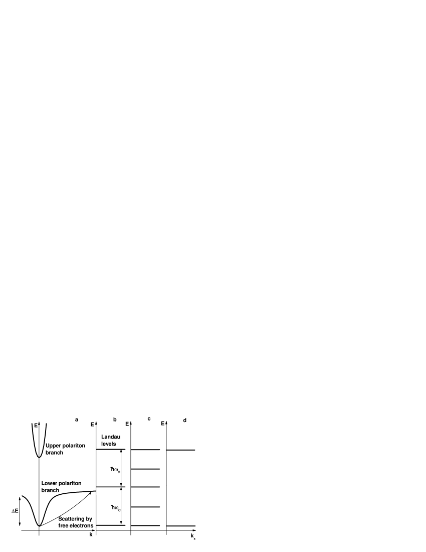
Figure 1: a) MC polariton dispersion curves; b),c),d) position of free QW electron Landau levels for the different magnitudes of the magnetic field. $\Delta E$ is the LP branch depth (separation between the free exciton level and the minima of the LP branch).

We calculate the MC polariton linewidth near the bottom of the LP branch due to the free QW electron scattering, neglecting the influence of the upper polariton branch states and localized exciton states. The spin distribution of particles is assumed to be isotropic. Polariton-electron scattering results from Coulomb interaction of an electron with an exciton which is a component of a polariton. For high enough temperature of the electron gas ($T\sim\Delta E$), polaritons from the region $k\approx 0$ scatter into the reservoir of the excitonlike states with high $k$ (Fig.1a). The probability for the polariton to leave the state with the wave vector $\vec{K}_{i}$ is calculated using the Fermi Golden rule:

$$\gamma_{\vec{\textbf{K}}_{i}}=4\pi\sum_{\vec{\textbf{k}}_{i},\vec{\textbf{k}}_{f},s}p_{s}\cdot|M_{\vec{\textbf{K}}_{i},\vec{\textbf{k}}_{i},\vec{\textbf{Q}},s}|^{2}\cdot F_{\epsilon_{i}}\cdot(1-F_{\epsilon_{f}})\cdot\delta(E_{f}+\epsilon_{f}-E_{i}-\epsilon_{i}),$$ (1)

where $\vec{\textbf{Q}}=\vec{\textbf{K}}_{f}-\vec{\textbf{K}}_{i}=\vec{\textbf{k}}_{i}-\vec{\textbf{k}}_{f}$; $\vec{\textbf{K}},\vec{\textbf{k}}$ are the wave vectors and $E,\epsilon$ are the energies of the polariton and the electron respectively; index “$i$” corresponds to the initial state, “$f$” corresponds to the final state; $s=\pm$ is the spin configuration of a free electron and an electron which is a component of an exciton: sign “$+$” corresponds to the triplet configuration, sign “$-$” corresponds to the singlet configuration; $p_{s}$ is the probability for the system to have the spin configuration $s$, for the isotropic spin distribution of particles $p_{+}=\frac{3}{4},p_{-}=\frac{1}{4}$ Landau ; $F_{\epsilon}=1/(e^{\frac{\epsilon-\mu}{T}}+1)$ is the Fermi-Dirac electron distribution function; $M_{\vec{\textbf{K}}_{i},\vec{\textbf{k}}_{i},\vec{\textbf{Q}},s}$ is the matrix element of the Coulomb potential of the polariton-electron interaction.

We use the following wave functions (WF) to calculate the matrix element $M_{\vec{\textbf{K}}_{i},\vec{\textbf{k}}_{i},\vec{\textbf{Q}},s}$:

$$|\vec{\textbf{K}},\vec{\textbf{k}}\rangle=(C_{K}\hat{a}_{\vec{\textbf{K}}}^{+}+X_{K}\hat{b}_{\vec{\textbf{K}}}^{+})\cdot\hat{c}_{\vec{\textbf{k}}}^{+}|0\rangle,$$ (2)

where $\hat{a}^{+},\hat{b}^{+},\hat{c}^{+}$ are the creation operators of a photon, an exciton, and an electron respectively; $C_{K},X_{K}$ are the Hopfield coefficients of a photon and an exciton respectively Hopfield ; Sermage . In Eq. (2), in brackets, is the polariton creation operator. The exciton creation operator is given by the following expression (we note that the exciton is in its ground state):

$$\hat{b}_{\vec{\textbf{K}}}^{+}=\sum_{\vec{\textbf{k}}_{0}}\phi_{\alpha\vec{\textbf{K}}-\vec{\textbf{k}}_{0}}\cdot\hat{c}_{\vec{\textbf{k}}_{0}}^{+}\hat{d}_{\vec{\textbf{K}}-\vec{\textbf{k}}_{0}}^{+},$$ (3)

where $\hat{d}^{+}$ is the hole creation operator; $\alpha$ is the ratio of electron and exciton effective masses; $\phi_{\vec{\textbf{k}}}=\sqrt{\frac{8\pi\lambda^{2}}{S}}\cdot(1+(\lambda k)^{2})^{-\frac{3}{2}}$ is the Fourier transform of the WF of the relative electron-hole motion in the QW exciton: $\phi(\vec{\rho})=\sqrt{\frac{2}{\pi\lambda^{2}}}\cdot e^{-\frac{\rho}{\lambda}}$; $\lambda$ is associated with the in-plane Bohr radius of the QW exciton; $S$ is the quantization area.

In fact, the WF (2) corresponding to the different wave vectors of the polariton and the electron are nonorthogonal. In Malpuech ; Ramon this nonorthogonality was disregarded and the resulting matrix element was nonunitary: $M_{\vec{\textbf{K}}_{i},\vec{\textbf{k}}_{i},\vec{\textbf{Q}},s}\neq M_{\vec{\textbf{K}}_{i}+\vec{\textbf{Q}},\vec{\textbf{k}}_{i}-\vec{\textbf{Q}},-\vec{\textbf{Q}},s}^{*}$. In our model, we simply discard the terms in the WF, responsible for the nonorthogonality of the WF. The matrix element is calculated as:

$$M_{\vec{\textbf{K}}_{i},\vec{\textbf{k}}_{i},\vec{\textbf{Q}},s}=X_{K_{i}}X_{|\vec{\textbf{K}}_{i}+\vec{\textbf{Q}}|}\cdot\langle 0|\sum_{\vec{\textbf{k}}_{2}\neq\vec{\textbf{k}}_{i}}\phi_{\alpha(\vec{\textbf{K}}_{i}+\vec{\textbf{Q}})-\vec{\textbf{k}}_{2}}\hat{c}_{\vec{\textbf{k}}_{i}-\vec{\textbf{Q}}}^{+}\hat{d}_{\vec{\textbf{K}}_{i}+\vec{\textbf{Q}}-\vec{\textbf{k}}_{2}}^{+}\hat{c}_{\vec{\textbf{k}}_{2}}^{+}\\ \times(\hat{V}_{ee}+\hat{V}_{eh})\sum_{\vec{\textbf{k}}_{1}\neq\vec{\textbf{k}}_{i}-\vec{\textbf{Q}}}\phi_{\alpha\vec{\textbf{K}}_{i}-\vec{\textbf{k}}_{1}}\hat{c}_{\vec{\textbf{k}}_{1}}^{+}\hat{d}_{\vec{\textbf{K}}_{i}-\vec{\textbf{k}}_{1}}^{+}\hat{c}_{\vec{\textbf{k}}_{i}}^{+}|0\rangle.$$ (4)

The discarding of sum components with $\vec{\textbf{k}}_{2}=\vec{\textbf{k}}_{i}$ and $\vec{\textbf{k}}_{1}=\vec{\textbf{k}}_{i}-\vec{\textbf{Q}}$ removes the above mentioned nonorthogonality of the WF Nonorthogonality . The electron-electron and electron-hole Coulomb interaction operators $\hat{V}_{ee},\hat{V}_{eh}$ are defined by the following expressions:

$$\hat{V}_{ee} = \frac{1}{2}\sum_{\vec{\textbf{k}}_{1},\vec{\textbf{k}}_{2},\vec{\textbf{q}}}V(q)\cdot\hat{c}_{\vec{\textbf{k}}_{1}+\vec{\textbf{q}}}^{+}\hat{c}_{\vec{\textbf{k}}_{2}-\vec{\textbf{q}}}^{+}\hat{c}_{\vec{\textbf{k}}_{2}}\hat{c}_{\vec{\textbf{k}}_{1}}$$ (5)

$$\hat{V}_{eh} = -\sum_{\vec{\textbf{k}}_{1},\vec{\textbf{k}}_{2},\vec{\textbf{q}}}V(q)\cdot\hat{c}_{\vec{\textbf{k}}_{1}+\vec{\textbf{q}}}^{+}\hat{d}_{\vec{\textbf{k}}_{2}-\vec{\textbf{q}}}^{+}\hat{d}_{\vec{\textbf{k}}_{2}}\hat{c}_{\vec{\textbf{k}}_{1}},$$ (6)

$$V(q) = \frac{4\pi e^{2}}{\varepsilon SL^{2}}\cdot\frac{e^{-Lq}-1+\frac{5(Lq)^{3}}{8\pi^{2}}+\frac{3(Lq)^{5}}{23\pi^{4}}}{q^{3}[1+(\frac{Lq}{2\pi})^{2}]^{2}},$$ (7)

where $V(q)$ is the Fourier transform of the Coulomb potential, which takes into account the finite QW width $L$ (the electron and hole transverse WF: $\sqrt{\frac{2}{L}}sin(\pi\frac{z}{L}),0<z<L$, QW is assumed to be infinitely deep); $e$ is the elementary charge; $\varepsilon$ is the dielectric susceptibility of the QW. For the details of calculating $V(q)$ one can refer to Ramon .

Using the anticommutation relation for the fermion operators one can find from Eq.(4) the scattering matrix element:

$$M_{\vec{\textbf{K}}_{i},\vec{\textbf{k}}_{i},\vec{\textbf{Q}},\pm}=X_{K_{i}}X_{|\vec{\textbf{K}}_{i}+\vec{\textbf{Q}}|}\cdot(M_{\vec{\textbf{K}}_{i},\vec{\textbf{k}}_{i},\vec{\textbf{Q}}}^{dir}\pm M_{\vec{\textbf{K}}_{i},\vec{\textbf{k}}_{i},\vec{\textbf{Q}}}^{exch}),$$ (8)

$$M_{\vec{\textbf{K}}_{i},\vec{\textbf{k}}_{i},\vec{\textbf{Q}}}^{dir}=V(Q)\cdot[\frac{1}{(1+(\frac{\beta}{2}\lambda Q)^{2})^{\frac{3}{2}}}-\frac{1}{(1+(\frac{\alpha}{2}\lambda Q)^{2})^{\frac{3}{2}}}],$$ (9)

$$M_{\vec{\textbf{K}}_{i},\vec{\textbf{k}}_{i},\vec{\textbf{Q}}}^{exch}=-\frac{2\lambda^{2}}{\pi}\int\frac{V(k)d^{2}k}{(1+\lambda^{2}(\vec{\textbf{k}}+\alpha\vec{\textbf{K}}_{i}-\vec{\textbf{k}}_{i}+\vec{\textbf{Q}})^{2})^{\frac{3}{2}}(1+\lambda^{2}(\vec{\textbf{k}}+\alpha\vec{\textbf{K}}_{i}-\vec{\textbf{k}}_{i}+\alpha\vec{\textbf{Q}})^{2})^{\frac{3}{2}}},$$ (10)

here $\beta=1-\alpha$ is the fraction of the effective mass of a hole in that of an exciton. One can easily check up that the obtained matrix element is unitary. Since the matrix element is calculated, one can calculate the linewidth using Eq.(1).

III Polariton-electron scattering in magnetic field

We use the similar formalism, as in the previous section, to calculate the polariton linewidth in a magnetic field perpendicular to the MC plane ($z$ axis). The field is assumed to be small and

$$a_{H}\gg\lambda,$$ (11)

where $a_{H}=\sqrt{\frac{\hbar c}{eB}}$ is the magnetic length, $B$ is the magnetic field magnitude, $c$ is the velocity of light.

Magnetic field makes discrete the energy spectrum of free electrons. We use here the Landau gauge for the vector potential $\vec{\textbf{A}}=(-By,0,0)$. The electron, hole and exciton WF are written as Landau :

$$\langle\vec{\textbf{r}}|\hat{\tilde{c}}_{n,k_{x}}^{+}|0\rangle = \frac{1}{\sqrt{a_{H}L_{x}}}\cdot e^{ik_{x}r_{x}}\cdot\varphi_{n}(\frac{r_{y}-a_{H}^{2}k_{x}}{a_{H}})$$ (12)

$$\langle\vec{\textbf{r}}|\hat{\tilde{d}}_{n,k_{x}}^{+}|0\rangle = \frac{1}{\sqrt{a_{H}L_{x}}}\cdot e^{ik_{x}r_{x}}\cdot\varphi_{n}(\frac{r_{y}+a_{H}^{2}k_{x}}{a_{H}})$$ (13)

$$\langle\vec{\textbf{R}},\vec{\rho}|\hat{\tilde{b}}_{\vec{\textbf{K}}}^{+}|0\rangle = \frac{1}{S}\cdot e^{iK_{x}R_{x}+i(K_{y}+\frac{\rho_{x}}{a_{H}^{2}})R_{y}}\tilde{\phi}(\vec{\rho}),$$ (14)

where $\varphi_{n}(x)=\frac{1}{\sqrt{\sqrt{\pi}2^{n}n!}}\cdot e^{-\frac{x^{2}}{2}}H_{n}(x)$ is the one-dimensional harmonic oscillator WF, $H_{n}(x)$ are the Hermite polynomials; $L_{x}$ is the quantization length in the $x$ direction; $\vec{\textbf{R}}$ is the coordinate of the center of mass of the exciton; $\vec{\rho}$ is the coordinate of the electron-hole relative motion in the exciton; $\tilde{\phi}(\vec{\rho})$ is the relative motion WF in a magnetic field. Thus we characterize the free electron motion by the Landau level number $n$ and by the $x$-component of the pseudomomentum $k_{x}$, exciton motion by the total pseudomomentum $\vec{\textbf{K}}$ Johnson . Taking into account (11) we can neglect the influence of the magnetic field on the electron-hole relative motion in an exciton and assume $\tilde{\phi}(\vec{\rho})=\sqrt{\frac{2}{\pi\lambda^{2}}}\cdot e^{-\frac{\rho}{\lambda}}$. Hence we neglect the change of the Raby splitting, the polariton dispersion law and the Hopfield coefficients due to the magnetic field. Precision of such an approximation is of order of $\frac{\lambda^{2}}{a_{H}^{2}}$ Johnson .

Eq. (1) now reads as

$$\gamma_{\vec{\textbf{K}}_{i}}=4\pi\sum_{n_{i},n_{f},k_{ix},\vec{\textbf{Q}},s}p_{s}\cdot|\tilde{M}_{\vec{\textbf{K}}_{i},n_{i},n_{f},\vec{\textbf{Q}},s}|^{2}F_{n_{i}}\cdot(1-F_{n_{f}})\cdot\delta(E_{f}-E_{i}-\hbar\omega_{c}(n_{f}-n_{i})),$$ (15)

here the summation is done not only over the initial and final electron states and the spin orientation but also over the $y$-component of the final polariton pseudomomentum $K_{fy}$ since it is not fixed by the conservation law. In Eq. (15) $\omega_{c}=\frac{eB}{m_{e}c}$ is the electron cyclotron frequency; $F_{n}=1/(e^{\frac{\hbar\omega_{c}(n+\frac{1}{2})-\mu}{T}}+1)$, Zeeman splitting of the electron and polariton energy levels is neglected and $p_{s}$ in Eq. (15) corresponds to the isotropic spin distribution. As a result of the translational symmetry, the absolute value of the matrix element is not dependent on the $x$-component of the initial pseudomomentum of the electron $k_{ix}$, and the summation over $k_{ix}$ gives the constant factor $\frac{S}{2\pi a_{H}^{2}}$, which is a number of states corresponding to the one Landau level.

As in the previous section, we use the following WF to calculate the polariton-electron interaction matrix element:

$$|\vec{\textbf{K}},n,k_{x}\rangle=(C_{K}\hat{a}_{\vec{\textbf{K}}}^{+}+X_{K}\hat{\tilde{b}}_{\vec{\textbf{K}}}^{+})\cdot\hat{\tilde{c}}_{n,k_{x}}^{+}|0\rangle$$ (16)

(the electron and exciton creation operators in (2) are replaced by the corresponding operators in a magnetic field). The WF nonorthogonality is treated as in the previous section. After the some lengthly calculations, taking into account (11), one can find the scattering matrix element in a magnetic field:

$$\tilde{M}_{\vec{\textbf{K}}_{i},n_{i},n_{f},\vec{\textbf{Q}},s}=\frac{a_{H}^{2}}{\sqrt{2\pi}}\int\varphi_{n_{i}}(a_{H}k_{y})\varphi_{n_{f}}(a_{H}(k_{x}-Q_{x}))e^{-ia_{H}^{2}k_{x}(k_{y}-Q_{y})}\cdot M_{\vec{\textbf{K}}_{i},\vec{\textbf{k}},\vec{\textbf{Q}},s}d^{2}k,$$ (17)

where $M_{\vec{\textbf{K}}_{i},\vec{\textbf{k}},\vec{\textbf{Q}},s}$ is calculated using Eq.(8)-(10). $k_{ix}$ arises only in the phase factor, which does not contribute to the scattering probability and is omitted here.

Precision of the above calculations is of order of $\frac{\lambda^{2}}{a_{H}^{2}}$.

IV Results and discussion

The numerical calculations was performed for the GaAs based MC with the QW of width $L=75\AA$ and with Raby splitting $4$ meV. The exciton Bohr radius $\lambda=150\AA$, the ratio of electron and exciton effective masses $\alpha=0.17$, the electron gas concentration in the QW $n_{e}=10^{9}$ cm^-2.

Figure 2: Dependence of the polariton linewidth on the electron gas temperature for zero exciton-photon detuning and $B=0$.

Fig.2 shows the calculated temperature dependence of the polariton linewidth for zero exciton-photon detuning ($E_{ph}(k=0)-E_{ex}(k=0)=0$), corresponding to $\Delta E=2$ meV, without magnetic field. For small temperatures ($T\ll\Delta E$) the polariton-electron scattering is noneffective since polaritons can not receive from electrons sufficient energy to get to the reservoir with high $k$ (Fig.1a). The polariton linewidth increases with increasing temperature and after reaching a maximum slowly decreases. Such a decrease for high temperatures is due to the smaller exchange scattering matrix element for high energy electrons (see Eq. (10)).

Figure 3: Dependence of the polariton linewidth on the magnetic field magnitude for zero exciton-photon detuning and $T=20$. The top scale shows the separation between Landau levels. Arrow indicates the value of the polariton linewidth, calculated for $B=0$ and $T=20K$ (see fig.2).

Fig.3 shows the calculated magnetic field dependence of the polariton linewidth for zero exciton-photon detuning and $T=20$K. Maximums in Fig.3 correspond to $\hbar\omega_{c}(n_{i}-n_{f})\gtrapprox\Delta E$ (see the top scale in the figure and note that $\Delta E=2$ meV). First maximum corresponds to $n_{i}-n_{f}=1$ (Fig.1b), second maximum corresponds to $n_{i}-n_{f}=2$ (Fig.1c) etc. Thus polariton-electron scattering rate can be not only decreased, but also increased by a magnetic field perpendicular to the MC plane. For the magnetic fields, for which $\hbar\omega_{c}$ considerably exceeds the LP branch depth (Fig.1d), the polariton linewidth monotonically decreases with the increasing field magnitude (Fig.3). The last effect was observed experimentally for $B=7$ T Qarry . Unfortunately there is no experimental data concerning the MC polariton-electron scattering in weak magnetic fields known.

Similar oscillatory magnetic field dependence of scattering rate was derived theoretically for electron-electron scattering between two QW subbands Kempa . Although the difference of the considered systems here and in Kempa , the nature of the scattering rate oscillations is the same.

- (1) C. Weisbuch, M. Nishioka, A. Ishikawa, et al., Phys. Rev. Lett. 69, 3314 (1992).
- (2) R. Butté, G. Delalleau, A.I. Tartakovskii, et al., Phys. Rev. B 65, 205310 (2002).
- (3) R.M. Stevenson, V.N. Astratov, M.S. Skolnick, et al., Phys. Rev. Lett. 85, 3680 (2000).
- (4) D.N. Krizhanovskii, A.I. Tartakovskii, M.N. Makhonin, et al., Phys. Rev. B 70, 195303 (2004).
- (5) D.N. Krizhanovskii, M.N. Makhonin, A.I. Tartakovskii, et al., Zh. Eksp. Teor. Fiz. 100, 126 (2005).
- (6) G. Malpuech, A. Kavokin, A. Di Carlo, et al., Phys. Rev. B 65, 153310 (2002).
- (7) P.G. Lagoudakis, M.D. Martin, J.J. Baumberg, et al., Phys. Rev. Lett. 90, 206401 (2003).
- (8) A.I. Tartakovskii, D.N. Krizhanovskii, G. Malpuech, et al., Phys. Rev. B 67, 165302 (2003).
- (9) J.J. Hopfield, Phys. Rev. 112, 1555 (1958).
- (10) B. Sermage, S. Long, I. Abram, et al., Phys. Rev. B 53, 16516 (1996).
- (11) G. Ramon, A. Mann and E. Cohen, Phys. Rev. B 67, 045323 (2003).
- (12) In the limit , the orthogonal WF could be chosed naturally, if one would use the WF of an electron, propagating in the field of an infinitly heavy hole instead of the WF of a free electron. One can proove directly, that the matrix element derived by such a way coinsides with the matrix element calculated using the WF nonorthogonality removal in the limit .
- (13) L.D. Landau and E.M. Lifshitz, “Quantum mechanics”, 3rd ed.,Pergamon, New York (1977).
- (14) B.R. Johnson, J.O. Hirschfelder and Kuo-Ho Yang, Rev. Mod. Phys. 55, 109 (1983).
- (15) K. Kempa, Y. Zhou, J.R. Engelbrecht, et al., Phys. Rev. B 68, 085302 (2003).
- (16) A. Qarry, R. Rapaport, G. Ramon, et al., Physica E 12, 528 (2002).