On the free energy within the mean-field approximation

Abstract

We compare two widespread formulations of the mean-field approximation, based on minimizing an appropriately built mean-field free energy. We use the example of the antiferromagnetic Ising model to show that one of these formulations does not guarantee the existence of an underlying variational principle. This results in a severe failure where straightforward minimization of the corresponding mean-field free energy leads to incorrect results.

In statistical physics the mean-field approximation is one of the most common and easy-to-use frameworks. It is also one of the most powerful, and often the only available one. It allows one to convert the study of a many-body problem of interacting degrees of freedom into that of independent degrees of freedom. There are several manners of performing a mean-field approximation. Our purpose is not to review them nor to discuss the corresponding well-documented pitfalls chandler ; diuetal ; goldenfeld ; lebellac ; yeomans ; parisi . Among those various mean-field versions, the one that is based on a rigorous variational principle plays a special role. Our purpose in the present note is to confront this rigorous, albeit cumbersome approach, with simpler and widely used formulations. We would like to analyze a hazardous ambiguity in the concept of free energy in those apparently more physical formulations which, to the best of our knowledge, has not been noted before. The reason why these conceptually erroneous statements that can be found in many places in the literature (diuetal , tuckerman ) have never been challenged is that pedagogical presentations are usually confined to the ferromagnetic Ising model, which has a scalar order parameter, and for which, somewhat luckily, the dangers we will point out remain hidden.

We have chosen to illustrate our discussion with the anti-ferromagnetic Ising model on a two-dimensional square lattice of $N$ sites, say with periodic boundary conditions rque , for our discussion would be pointless with a scalar order parameter. The $N$ spins $s_{i}=\pm 1$, $i=1,...,N$ are interacting according to the following Hamiltonian:

$${\cal H}=+J\sum_{\langle i,j\rangle}s_{i}s_{j}$$ (1)

where the sum $\sum_{\langle i,j\rangle}$ runs over the $2N$ distinct pairs of nearest neighbour sites, and where the constant $J>0$ is the anti-ferromagnetic coupling. The high temperature phase of the system is paramagnetic ($m_{i}=\langle s_{i}\rangle$ vanishes). As the temperature is decreased below the so called Néel temperature $T_{N}$ anti-ferromagnetic order sets in: The spins align in opposite directions on two square sub-lattices, as shown in Figure 1. The lattice sites are conveniently divided into two subsets $a$ and $b$, as already depicted on Figure 1.

We begin with a reminder of the variational formulation of the mean-field approximation (route 1), and then present a more standard approach (route 2) and the accompanying difficulties in interpreting the related free energy.

Route 1: Variational procedure. The idea binneydowrickfischernewman ; peierls ; feynman is to introduce a trial Hamiltonian ${\cal H}_{\text{mf}}$ depending on the original degrees of freedom $\{s_{i}\}$ and on two parameters $m_{a}$ and $m_{b}$ the physical meaning of which will become clear later. An intuitive choice for ${\cal H}_{\text{mf}}$ is

$${\cal H}_{\text{mf}}=+4Jm_{b}\sum_{i\in a}s_{i}+4Jm_{a}\sum_{j\in b}s_{j}$$ (2)

Then one splits ${\cal H}$ into

$${\cal H}={\cal H}_{\text{mf}}+({\cal H}-{\cal H}_{\text{mf}})$$ (3)

so that the free energy $F$ of the system reads

$$F=F_{\text{mf}}-k_{\hbox{\tiny B}}T\ln\langle\hbox{e}^{-\beta({\cal H}-{\cal H}_{\text{mf}})}\rangle_{\text{mf}}.$$ (4)

Here, $\beta F_{\text{mf}}=-\log Z_{\text{mf}}$ where $Z_{\text{mf}}$ is the partition function associated to (2), $\beta=1/(k_{\hbox{\tiny B}}T)$ is the inverse temperature with $k_{\hbox{\tiny B}}$ the Boltzmann constant and the angular brackets $\langle...\rangle_{\text{mf}}$ denote an average using the Gibbs measure related to ${\cal H}_{\text{mf}}$, that is with weight $\exp(-\beta{\cal H}_{\text{mf}})$. The exponential being convex, one is led to the inequality

$$F\leq F_{\text{mf}}+\langle{\cal H}-{\cal H}_{\text{mf}}\rangle_{\text{mf}}.$$ (5)

Equation (5) often appears under the name of Bogoliubov inequality and may be used to find the best set of parameters $m_{a}$ and $m_{b}$ that render $\phi(m_{a},m_{b})=F_{\text{mf}}+\langle{\cal H}-{\cal H}_{\text{mf}}\rangle_{\text{mf}}$ minimum, that is as close as possible to the exact free energy $F$ rque2 . It is important to note here that the best approximation for $F$ is not $F_{\text{mf}}(m_{a},m_{b})$ but $\phi(m_{a},m_{b})$. Using that $\langle s_{i\in a}\rangle_{\text{mf}}=-\tanh 4\beta Jm_{b}$ and $\langle s_{j\in b}\rangle_{\text{mf}}=-\tanh 4\beta Jm_{a}$ we arrive at

$$\begin{split}\beta\phi(m_{a},m_{b})=&\overbrace{\frac{N}{2}\Big{[}-\ln\left(4\cosh 4\beta Jm_{a}\cosh 4\beta Jm_{b}\right)}^{\beta F_{\text{mf}}}\\ &+4\beta J\tanh 4\beta Jm_{a}\tanh 4\beta Jm_{b}\\ &+4\beta J\left(m_{a}\tanh 4\beta Jm_{a}+m_{b}\tanh 4\beta Jm_{b}\right)\Big{]}\end{split}$$ (6)

Extremizing $\phi$ leads to the set of equations

$$\frac{\partial\phi}{\partial m_{a}}=0,\;\frac{\partial\phi}{\partial m_{b}}=0$$ (7)

$$\Rightarrow m_{a}=-\tanh 4\beta Jm_{b},\;m_{b}=-\tanh 4\beta Jm_{a}$$ (8)

The latter system of equations has a unique solution $m_{a}=m_{b}=0$ at $\beta\leq\beta_{N}=\frac{1}{4J}$ ($T_{N}=4J/k_{\hbox{\tiny B}}$) and possesses an additional set of two nonzero solutions for $\beta>\beta_{N}$ ($T_{N}$ is identified as the Néel temperature). In the high temperature phase the paramagnetic solution $m_{a}=m_{b}=0$ becomes the global minimum of $\phi$, just as the nonzero solution $m_{a}=-m_{b}\neq 0$ does in the low temperature phase (one can verify that the matrix of the second derivatives of $\phi$ is positive definite at those extrema). Note also that for $\beta>\beta_{N}$ the paramagnetic state is a saddle point of $\phi$ with the unstable direction along the $m_{a}=-m_{b}$ line (see Figure 2). Right at the minimum, the expression of $\phi$ reads

$$\phi(m_{a},m_{b})=F_{\text{mf}}-2NJm_{a}m_{b}$$ (9)

where $m_{a}$ and $m_{b}$ are the solutions to the system in (7).

At this stage we have simply postulated a trial Hamiltonian ${\cal H}_{\text{mf}}$ without providing much of a physical motivation. It is a posteriori clear that ${\cal H}_{\text{mf}}$ describes a system of independent spins in an external magnetic field. For spin $s_{i}$ of sub-lattice $a$ this magnetic field is interpreted as the mean magnetization resulting from the four nearest neighbors on sub-lattice $b$, as is confirmed by the fact that at the minimum of $\phi$ one can indeed verify that

$$\langle s_{\in a}\rangle_{\text{mf}}=-\tanh 4\beta Jm_{b}=m_{a},\;\langle s_{\in b}\rangle_{\text{mf}}=m_{b}$$ (10)

In practice, however the variational procedure is not physically transparent and is mathematically rather heavy. Furthermore it must be supplemented with a reasonable input of physical intuition when postulating a trial Hamiltonian, lest the outcome of the calculation should be dull. Hence, for all these reasons, in spite of $\phi(m_{a},m_{b})$ being a bona fide mean-field free energy, it is rarely used in standard courses. The purpose of the sequel is to present an alternative and widely used formulation of the mean-field approximation diuetal ; tuckerman , which at first glance appears more satisfactory on physical grounds, but that conceals a number of hazards that we wish to point out.

Alternative formulation. Replacing in the original Hamiltonian $\cal H$ the spins $s_{\ell}$ with $m_{a\hbox{\tiny~{}or }b}+\delta s_{\ell}$ and neglecting terms quadratic in the $\delta s_{\ell}$’s, we obtain our new mean-field Hamiltonian ${\cal H}^{\prime}_{\hbox{\tiny mf}}$:

$${\cal H}^{\prime}_{\hbox{\tiny mf}}=-2NJm_{a}m_{b}+4Jm_{b}\sum_{i\in a}s_{i}+4Jm_{a}\sum_{j\in b}s_{j}.$$ (11)

In the present formulation, the mean-field approximation can be viewed as neglecting correlations between nearest neighbour spin fluctuations. The difference between the above ${\cal H}^{\prime}_{\hbox{\tiny mf}}$ and the ${\cal H}_{\hbox{\tiny mf}}$ that appears in (2) lies in the additional constant term $-2NJm_{a}m_{b}$ that features a temperature dependence through the magnetizations $m_{a}$ and $m_{b}$ that must carefully be kept track of. It is easily checked that following the above variational procedure route 1 with ${\cal H}^{\prime}_{\hbox{\tiny mf}}$ instead of ${\cal H}_{\hbox{\tiny mf}}$ leads to the same results rque2 . At this stage, another route can be followed, that differs from the variational procedure. We decompose this second route into two steps.

Route 2a: Self-consistency. From the mean-field Hamiltonian ${\cal H}^{\prime}_{\hbox{\tiny mf}}$ it is easy to deduce both the mean-field partition function $Z^{\prime}_{\hbox{\tiny mf}}$ and the average magnetization. We find

$$Z^{\prime}_{\hbox{\tiny mf}}=2^{N}\hbox{e}^{2N\beta Jm_{a}m_{b}}(\cosh(4\beta Jm_{a})\cosh(4\beta Jm_{b}))^{N/2}$$ (12)

and

$$m_{a}=\langle s_{i\in a}\rangle=\frac{1}{Z^{\prime}_{\hbox{\tiny mf}}}\sum_{\{s_{\ell}\}}s_{i}\hbox{e}^{-\beta{\cal H}^{\prime}_{\hbox{\tiny mf}}}=-\tanh(4J\beta m_{b})$$ (13)

$$m_{b}=\langle s_{j\in b}\rangle=-\tanh(4J\beta m_{a})$$ (14)

This system of equations is exactly the one found in (10). The self-consistency equations (13) and (14) have only the paramagnetic solution when $T\geq T_{N}$, while a nonzero solution continuously develops as $T$ is lowered below $T_{N}$. It is then argued that below $T_{N}$, which is identified with the Néel temperature, the $m_{a}=m_{b}=0$ solution is unstable while the solution $m_{a}=-m_{b}\neq 0$ becomes stable and is the physically relevant one. Either more precise discussions about stability issues are discarded or one finds in standard textbooks the following assertion to justify the choice of the nonzero solution below $T_{N}$: It becomes stable below the Néel temperature (this is true), as can be checked by studying the minima of the free energy. This is this last sentence that we would now like to discuss.

Route 2b: Free energy landscape. From the expression of the partition function given in (12) one can easily deduce an expression for the free energy $\phi^{\prime}(m_{a},m_{b})$ as a function of the magnetizations on the two sub-lattices:

$$\begin{split}\phi^{\prime}(m_{a},m_{b})=&-k_{\hbox{\tiny B}}T\log Z^{\prime}_{\text{mf}}=N\Big{(}-2Jm_{a}m_{b}\\ &-\frac{1}{2\beta}\ln\left[4\cosh(4\beta Jm_{a})\cosh(4\beta Jm_{b})\right]\Big{)}\end{split}$$ (15)

We now express that we search for the states that minimize the free energy $\phi^{\prime}$

$$\frac{\partial\phi^{\prime}}{\partial m_{a}}=\frac{\partial\phi^{\prime}}{\partial m_{b}}=0$$ (16)

Within the framework of the simpler ferromagnetic case, this is precisely the wording adopted e.g. in diuetal . It is then usually commented that the equations (16) are equivalent to those obtained by resorting directly to the self-consistency conditions. A plot of the free energy landscape as a function of the order parameter usually follows. And indeed for $T<T_{N}$ it may be seen that the paramagnetic state becomes a global maximum of $\phi^{\prime}$ considered as a function of independent variables $(m_{a},m_{b})$.

However, below the Néel temperature, the nontrivial state $(m_{a},m_{b})$ deduced from (13) and (14) is simply neither a local nor a global minimum of the free energy $\phi^{\prime}(m_{a},m_{b})$:
(i) there exist other states, at the boundaries of the magnetization domain, that have a lower free energy;
(ii) $(m_{a},m_{b})$ as given by the nonzero solution of (13) and (14) does not even correspond to a local minimum.
It is instructive to examine the shape of the free energy landscape as a function of the order parameter components $(m_{a},m_{b})$, as plotted in Figure 3. We find that the state that globally minimizes the free energy $\phi^{\prime}$ is the fully ordered ferromagnetic $m_{a}=m_{b}=1$ state (or equivalently $m_{a}=m_{b}=-1$), whatever $0\leq T<T_{N}$. Furthermore, the anti-ferromagnetic state corresponds to a saddle point of the free energy landscape. This is best appreciated on Figure 4. With the chosen parameters the correct anti-ferromagnetic state has $m_{a}\simeq 0.77$. We have clearly come across an unexpected hazard of the mean-field approximation. Finally, note that by artificially dividing a regular ferromagnetic Ising model on a square lattice into two sub-lattices with independent average magnetizations, one would come across the same kind of problems for the mean-field free energy (the ferromagnetic state would become a saddle-point, the global minimum would correspond to the fully anti-ferromagnetic state, etc.).

Discussion. We now come back to the variational formulation and we wish to underline that when one evaluates $\phi$ at its global minimum one finds that

$$\phi(m_{a},m_{b})=\phi^{\prime}(m_{a},m_{b})$$ (17)

where $m_{a}$ and $m_{b}$ are the functions of temperature solution to the system (13,14) or (10). This tells us that it is perfectly legitimate to follow route 2a using the numerical value of $\phi^{\prime}$ at the values given by (13,14) for finding the physical solution to the problem. In other words, route 2a with the further computation of $\phi$ for the self-consistent magnetizations is correct. However it should be prohibited to freely vary the magnetizations $m_{a}$ and $m_{b}$ as in route 2b to study the free-energy $\phi^{\prime}$ landscape and to rely on the latter landscape to discuss stability issues. There is indeed no variational principle underlying the derivation of $\phi^{\prime}$. This is at variance with the safe route 1 relying of $\phi$. This also means that route 2 can never be used to discuss metastability issues, even restricting to self-consistent magnetizations.

The inconsistency we have brought forth for route 2b appears only when the mean-field order parameter is not a scalar (as is the case in the ferromagnetic model): Ordering phenomena on more complex substructures of the original lattice would inevitably lead to similar results. The key point in our second formulation of the mean-field approximation (route 2) is that by their very definition, $m_{a}$ and $m_{b}$ are the average magnetizations: They cannot be considered as freely varying variables. They are functions of the temperature determined by the self-consistency equations. It is curious to note that the physical solution ($m_{a},m_{b}$) to the problem (which is by definition a minimum of $\phi$) corresponds to a saddle point of the function $\phi^{\prime}$.

Therefore we would like to conclude by warning that there is in principle no physical meaning to the mean-field free energy $\phi^{\prime}$ seen as a function of a freely varying order parameter. Comparing mean-field free energies is meaningful only for solutions of the self-consistency equations. We have shown this below the Néel temperature, but similar problems arise in the high-temperature limit. Indeed, expanding the free energy Eq. (15) in the vicinity of $\beta=0$ yields $\phi^{\prime}_{\hbox{\tiny mf}}\simeq-2JNm_{a}m_{b}$ from which one could be tempted to conclude erroneously that the stable state is fully ferromagnetic when it is of course paramagnetic!

Figure 1: A two dimensional anti-ferromagnet, for $T\ll T_{N}$. The spins align almost perfectly in opposite directions on two sub-lattices $a$ and $b$ of the original lattice.

Figure 2: Plot of the trial free energy $\phi(m_{a},m_{b})$ at $T=2.2J/k_{\hbox{\tiny B}}<T_{N}$ as a function of $m_{a}$ along the $m_{a}=-m_{b}$ direction. Note the presence of degenerate global minima at finite magnetization.

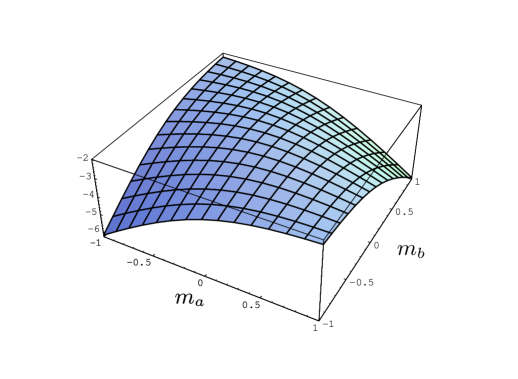
Figure 3: Plot of the dimensionless free energy $\phi^{\prime}_{\hbox{\tiny mf}}/(JN)$ as a function of $m_{a}$ and $m_{b}$ in $[-1,1]^{2}$, below the Néel temperature at $T=3\,T_{N}/4$.

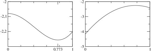
Figure 4: Plot of the dimensionless free energy $\phi^{\prime}_{\hbox{\tiny mf}}/(JN)$ as a function of $m_{a}$ along the $m_{a}=-m_{b}$ line (left) and along the perpendicular direction crossing the saddle point at $m_{a}=-m_{b}\simeq 0.77$ (right). Same parameters as in Fig. 3 .

References

- (1) D. Chandler, Introduction to Modern Statistical Mechanics (Oxford University Press, 1987).
- (2) B. Diu, C. Guthmann, D. Lederer and B. Roulet, Physique statistique (Herrmann, 1989).
- (3) N. Goldenfeld, Lectures on Phase Transitions and the Renormalization Group (Perseus Books, 1992).
- (4) M. Le Bellac, Quantum and Statistical Field Theory (Oxford University Press, 1992).
- (5) J.M. Yeomans, Statistical Mechanics of Phase Transitions (Clarendon Press, 1993).
- (6) G. Parisi, Statistical Field Theory (Addison Wesley 1988).
- (7) M.E. Tuckerman, online course accessible at http://www.nyu.edu/classes/tuckerman/stat.mech /lectures/lecture_26/node1.html
- (8) In the present case, the model is exactly solvable by mapping it onto its ferromagnetic counterpart, for which the solution may be found in L.D. Landau and E.M. Lifshitz, Statistical Physics (Pergamon Press, 1959). Yet, we use it as a pedagogical testbench.
- (9) J.J. Binney, N.J. Dowrick, A.J. Fischer and M.E.J. Newman, The theory of critical phenomena. An introduction to the renormalization group (Oxford University Press, 1992).
- (10) R.P. Feynman, Phys. Rev. 97, 660 (1955).
- (11) R. Peierls, Phys. Rev. 54, 918 (1934).
- (12) We note that the Bogoliubov bound [right hand side of Eq. (5)] is the same for all trial Hamiltonians of the form where is an arbitrary function.