Percolation in the Harmonic Crystal and Voter Model in Three Dimensions

Abstract

We investigate the site percolation transition in two strongly correlated systems in three dimensions: the massless harmonic crystal and the voter model. In the first case we start with a Gibbs measure for the potential, $U=\frac{J}{2}\sum_{<x,y>}\left(\phi(x)-\phi(y)\right)^{2}$, $x,y\in\mathbb{Z}^{3}$, $J>0$ and $\phi(x)\in\mathbb{R}$, a scalar height variable, and define occupation variables $\rho_{h}(x)=1,(0)$ for $\phi(x)>h(<h)$. The probability $p$ of a site being occupied, is then a function of $h$. In the voter model we consider the stationary measure, in which each site is either occupied or empty, with probability $p$. In both cases the truncated pair correlation of the occupation variables, $G(x-y)$, decays asymptotically like $|x-y|^{-1}$. Using some novel Monte Carlo simulation methods and finite size scaling we find accurate values of $p_{c}$ as well as the critical exponents for these systems. The latter are different from that of independent percolation in $d=3$, as expected from the work of Weinrib and Halperin [WH] for the percolation transition of systems with $G(r)\sim r^{-a}$ [A. Weinrib and B. Halperin, Phys. Rev. B 27, 413 (1983)]. In particular the correlation length exponent $\nu$ is very close to the predicted value of $2$ supporting the conjecture by WH that $\nu=\frac{2}{a}$ is exact.

I Introduction

A translation invariant ergodic system of point particles on a lattice, say $\mathbb{Z}^{d}$, in which each site is occupied with probability $p$, $0\leq p\leq 1$, is said to percolate when it contains an infinite cluster of occupied sites, connected by nearest neighbor bonds. This event satisfies the zero/one law, i.e. the probability that the system percolates is either zero or one  [1, 2]. For the case in which the sites are independent the transition from the non-percolating state for $p<p_{c}$ and the percolating one for $p>p_{c}$ is one of the simplest examples of critical phenomena. The probability that a given site, say the origin, is connected to infinity, i.e. is part of the infinite cluster, is zero for $p<p_{c}$ and strictly positive for $p>p_{c}$ [1, 2]. Much is known rigorously and even more from computer simulations and renormalization group calculations, about the nature of the percolation transition in the independent case. In particular it is known rigorously that $p_{c}$ is strictly greater than zero and less than one for $d\geq 2$ with $p_{c}(d)$ a decreasing function of $d$, etc. We also know explicitly or have bounds for some of the various exponents associated with the divergence of different quantities, e.g. the mean finite cluster size, when $p\rightarrow p_{c}$. We even know exactly the scaling limit of the shape of the critical cluster on the triangular lattice  [3].
It is generally believed that the critical properties, e.g. exponents, for independent percolation, but not $p_{c}$, are universal: they do not depend on the particular lattice but only on the dimensionality of the problem. The exponents are also believed not to be changed when one considers systems for which the occupation probabilities for different sites are not independent, as long as the correlations between occupied sites decay rapidly, say exponentially  [4].
Less is known about the percolation transition when there are long range correlations between occupied sites, e.g. when the correlations decay as a power law. Such power law decays occur in many physical systems and the nature of the percolation transition in such systems has come up recently in the study of two dimensional turbulence  [5], and of porous media, such as gels  [6].
In a seminal work Weinrib and Halperin  [7, 4] argued that the critical exponents of the percolation transition should depend only on the decay of the pair correlation $G(r)$ in such systems. In particular for $G(r)\sim r^{-a}$ the transition should be in a universality class which depends only on $a$ and $d$. Their analysis was based on considering the variance of the particle density in a region of volume $\xi^{d}$, where $\xi$ is the percolation correlation length which diverges as $p\nearrow p_{c}$. They found that if $a<d$ these correlations are relevant if $a\nu-2<0$. Here $\nu$ is the critical exponent which describes the divergence of the percolation correlation length $\xi$, e.g. the average radius of gyration of the clusters in the independent percolation problem as $p\nearrow p_{c}$, i.e. $\xi(p)\sim(p_{c}-p)^{-\nu}$. Weinrib and Halperin argued that systems that satisfy the above criteria belong to a new universality class for which the percolation correlation length exponent is $\nu_{long}=\frac{2}{a}$  [7, 4]. They also checked this using a renormalization group double expansion in $\epsilon=6-d$ and in $\delta=4-a$. While the computations of WH were done only in the one loop approximation the exponent $\nu_{long}$ was conjectured to be exact  [7, 4].
As pointed out by WH their results are consistent with those based on renormalization group ideas, both in real and momentum space, on the percolation of like-pointing Ising type spins at the critical point, see  [7] and references in there. There have also been some numerical tests of the WH predictions. For $d=2$ Prakash et al. [8] have carried out Monte Carlo simulations for percolation on artificially generated power law correlated occupation probabilities on $\mathbb{Z}^{2}$. This study confirmed the predictions of Weinrib and Halperin. The only direct check of the WH prediction in $d=3$ we are aware of is in  [6] where the authors introduced a bond percolation model in $\mathbb{Z}^{3}$, called Pacman percolation. They argued that the pair correlation for their model decays as $r^{-a}$, with a close to 1, and obtained critical exponents which are consistent with WH, but since $a$ was not known exactly the results are not fully conclusive.
In this paper we study the percolation transition in three dimensions for two systems in which the long range correlations arise naturally from the microscopic dynamics: the massless harmonic crystal and the voter model on $\mathbb{Z}^{3}$. Both of these systems are known rigorously to have $G(r)\sim r^{-1}$. They also have other similarities but are intrisicaly quite different. The existence and nature of the percolation transition in these systems is of interest in their own right. Using Monte Carlo simulations and finite size scaling we find the $p_{c}$ for both models. We also find that both models have the same critical exponents as expected from the WH predictions of a long range percolation universality class.
For the massless harmonic crystal in $\mathbb{Z}^{d}$ we define site x to be occupied if the scalar displacement field $\phi(x)$ is greater than some preassigned value $h$ and empty if $\phi(x)<h$. Percolation then corresponds to the existence of an infinite level set contour for $\phi(x)<h$. The existence of percolation threshold, i.e. $0<p_{c}<1$, was proven by Bricmont, Lebowitz and Maes [9] for $d=3$. There are however no previous calculations (known to us) concerning the actual value of $p_{c}$ or of the critical exponents for this system. One expects intuitively that the $p_{c}$ will be smaller than the $p_{c}$ for independent percolation ,c.f.  [8], but we know of no proof for this. Similarly a proof that $p_{c}>0$ for the harmonic crystal in $d>3$, or for the an-harmonic crystal in $d\geq 3$ is still an open problem  [10]. For $d\leq 2$, $\phi(x)$ is for any $h$, either plus or minus infinity, with probability 1, when the size of the system goes to infinity. Thus either all sites are occupied or all sites are empty.
The voter model, often used for modeling various sociological and biological phenomena , is a lattice system in which a site $x$ is occupied or empty according to whether the “voter” living there belongs to party A or B. Voters change their party affiliations according to a well defined stochastic dynamics  [11]. The stationary state of this model is not known explicitly but many of its properties are known exactly. In particular it has many features in common with the harmonic crystal. Like the harmonic crystal, the stationary state of the voter model is trivial in $d\leq 2$; all sites occupied or all sites empty. On the other hand any $p$ is possible on $\mathbb{Z}^{d}$ for $d\geq 3$, where the truncated pair correlation decays, as it does for the harmonic crystal, like $r^{-1}$. No proof of the existence of a $p_{c}>0$ is known for this system, i.e. the system could in principle percolate for arbitrary small $p$. For examples of systems where $p_{c}\leq\epsilon$ for any $\epsilon>0$ see  [12].
The outline of the rest of the paper is as follows. In Section 2 we present the simulation methods and results the massless harmonic crystal. In particular we find $p_{c}=0.16\pm 0.01$. In section 3 we study the voter model. We present a new efficient algorithm for simulating this model and report the results from its implementation. We find in particular that $p_{c}=0.10\pm 0.01$ compared with a $p_{c}\cong 0.16$ obtained in  [13] using a less reliable method. We conclude the paper with a brief discussion of some open problems.

II The Harmonic Crystal

II.1 Formulation

Let $x\in\mathbb{Z}^{d}$ designate the sites of a d-dimensional simple cubic lattice and $\phi(x)$ be the scalar displacement field at site $x$. The interaction potential in a box $\Lambda$ with specified boundary conditions (b.c.), e.g. $\phi(x)=0$ for $x$ on the boundary of $\Lambda$, has the form

$$U=\frac{1}{2}J\sum_{<x,y>}\left(\phi(x)-\phi(y)\right)^{2}+\frac{1}{2}M^{2}\sum\phi(x)^{2}\equiv\frac{1}{2}\sum_{x,y}\phi(x)C^{-1}(x,y)\phi(y)$$ (1)

where $J>0$ and $M\geq 0$, $<x,y>$ indicates nearest neighbor pairs, $|x-y|=1$, on $\mathbb{Z}^{d}$. The sum is over all sites in $\Lambda$ with the specified b.c. The Gibbs equilibrium distribution of the $\{\phi(x)\}$ at a temperature $\beta^{-1}$, $\mu^{M}_{\Lambda}(\{\phi(x)\})=Z^{-1}_{M,\Lambda}=e^{-\beta U}$ is then Gaussian with a covariance matrix $\beta\mathbf{C}$ which is well defined for $M>0$.
The infinite volume limit Gibbs measure $\mu^{M}$ obtained when $\Lambda\nearrow\mathbb{Z}^{d}$ is ,for $M>0$ ,translation invariant, with $<\phi(x)>=0$ and is independent of the boundary conditions  [14]. When $M\rightarrow 0$ , $\mu^{M}$ does not exist for $d\leq 2$ [14]. This is due to the fact that the fluctuations of the field, e.g $<\phi(x)^{2}>$, become unbounded for these dimensions. However, for $d\geq 3$ the Gibbs measure $\mu$ obtained as the limit of $\mu_{M}$ when $M\rightarrow 0$ is well defined. (It is the same as the infinite volume limit of the measure in a box with $M=0$ and prescribed boundary values $\phi(x)=0$). In this limit the pair correlations between different sites have the long distance behavior $\frac{1}{r^{d-2}}$, $r=|x-y|$ for $d>2$  [14].
Following [9] we define the occupation variable $\rho_{h}(x)$

$$\rho_{h}(x)=\begin{cases}1&\text{if $\phi(x)\geq h$}\\ 0&\text{if $\phi(x)<h$}\\ \end{cases}$$ (2)

and let $p=<\rho_{h}(x)>_{\mu^{M}}$, where the average is over the Gibbs measure $\mu^{M}$. We can also define a new measure $\hat{\mu}^{M}$ on the occupation variables $\rho_{h}(x)$=0,1 by a projection of $\mu^{M}$. All expectations involving a function of the occupation variables can be computed directly from $\hat{\mu}^{M}$. The correlations between the occupation variables have the same asymptotic decay properties as those of the field variables $\phi$,

$$\left<\rho_{h}(x)\rho_{h}(y)\right>_{\hat{\mu}^{M}}-p^{2}\sim\frac{e^{-|x-y|/{\xi_{M}}}}{|x-y|^{d-2}}\ \ \text{for $d>2$}$$ (3)

where $\xi_{M}\sim M^{-1}$ and the averages are with respect to $\hat{\mu}^{M}$(or $\mu^{M}$). In the limit $M\rightarrow 0$ the measure $\hat{\mu}$ has a pair correlation that decays like $r^{2-d}$ for $d>2$. We note that $\hat{\mu}$ is not Gibbsian for any summable potential, c.f  [15].

II.2 Results

Simulating the harmonic crystal on finite lattices is easy, the elements in a discrete Fourier transform of a harmonic crystal are independently distributed Gaussian random variables with easily computed variances [16]. We consider the system on a lattice with periodic boundary conditions and exclude the zero mode. This is essentially equivalent to fixing $\left<\phi\right>=0$.
There are many methods for obtaining the percolation threshold using data obtained from simulations on finite systems [1]. We used the method employed in  [17, 13]. For a cube of linear size $L$ let

$$\Gamma_{L}=\left<\sum_{j}j^{2}n_{j}\right>$$ (4)

where $n_{j}$ is the number of clusters of $j$ sites, defined by the occupation variables $\rho_{h}(x)$, and the average is taken over a large number of samples obtained from simulation of the model. We calculate $\Gamma_{L}$ for different sizes $L$ and concentration of occupied sites $p$ defined as in (2).
One expects  [1, 17, 18] that for large $L$,and $(p_{c}-p)\ll 1$, $\Gamma_{L}$ should have a finite size scaling form,

$$L^{-d}\Gamma_{L}\sim L^{\frac{\gamma}{\nu}}F(L^{\frac{1}{\nu}}(p-p_{c}))+\mbox{corrections to scaling},$$ (5)

where $\gamma$ is the critical exponent for the divergence as $p\nearrow p_{c}$ of the second moment of the cluster size distribution, defined as the limit $L\rightarrow\infty$ of $\frac{\Gamma_{L}}{L^{d}}$. Corrections to scaling should go to zero for $L\rightarrow\infty$.
For $p>p_{c}$, for an infinite system the second moment of the cluster size distribution can be defined by excluding the infinite cluster. This diverges with a critical exponent $\gamma^{{}^{\prime}}$ for $p\searrow p_{c}$. The finite system analog is $\frac{\Gamma_{L}^{{}^{\prime}}}{L^{d}}$ which is defined similarly to $\frac{\Gamma_{L}}{L^{d}}$ but not including the spanning cluster. $\Gamma_{L}^{{}^{\prime}}$ scales as

$$L^{-d}\Gamma_{L}^{{}^{\prime}}\sim L^{\frac{\gamma^{{}^{\prime}}}{\nu}}F^{{}^{\prime}}(L^{\frac{1}{\nu}}(p-p_{c}))+\mbox{corrections to scaling}.$$ (6)

It is believed that $\gamma^{{}^{\prime}}$ = $\gamma$.
According to finite size scaling theory the number of sites in the largest cluster in a finite system of linear size $L$, $P_{L}(p)$, scales for $|p-p_{c}|\ll 1$ as

$$P_{L}(p)\sim L^{d-\frac{\beta}{\nu}}G(L^{\frac{1}{\nu}}(p-p_{c}))+\mbox{corrections to scaling}$$ (7)

[1, 18], where $\beta$ is the critical exponent for the approach to zero of the fraction of sites belonging to the infinite cluster in an infinite system as $p\searrow p_{c}$. Using the hyper-scaling relation $d=2\frac{\beta}{\nu}+\frac{\gamma}{\nu}$ we see that (5), (6) and (7) lead to the scaling form (5) being valid for all $|p-p_{c}|\ll 1$ and large $L$. That is on a finite system we do not need to differentiate between $p<p_{c}$ or $p>p_{c}$, we may include all the clusters when calculating $\Gamma_{L}(p)$.
Assuming (5) is valid for $|p-p_{c}|\ll 1$ the ratio $R_{L}=\frac{\Gamma_{2L}}{\Gamma_{L}}$ should become independent of $L$, for large $L$, at $p=p_{c}$. Plotting these ratios as a function of $p$ for different sizes $L$ and looking for the intersection of these different curves then yields $p_{c}$. The value of the ratios at the intersection point of the $R_{L}$ curves should be equal to $2^{d+\frac{\gamma}{\nu}}$ giving us a way to measure $\frac{\gamma}{\nu}$. Moreover ,we also have

$$\frac{1}{\nu}=\frac{\log{\left(\frac{dR_{2L}}{dp}/\frac{dR_{L}}{dp}\right)}}{\log{2}}.$$ (8)

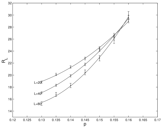
Figure 1: Plot of $R_{L}$ versus p for the $d=3$ massless harmonic crystal. We estimate $p_{c}=0.16\pm 0.01$

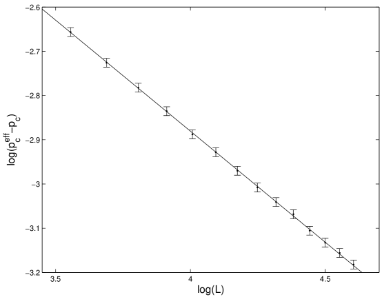
Figure 2: Plot of $\log(p_{c}^{eff}-p_{c})$ versus $\log(L)$. The slope if the straight line gives $\nu=2.00\pm 0.04$

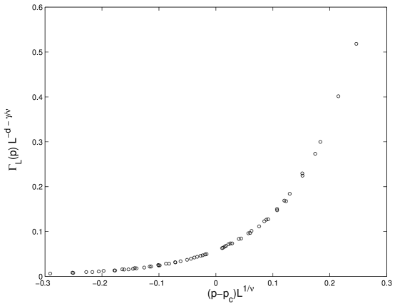
Figure 3: Plot of $\Gamma_{L}L^{-d-\frac{\gamma}{\nu}}$ versus $(p-p_{c})L^{\frac{1}{\nu}}$ for the $d=3$ massless harmonic crystal for $p_{c}=0.16$, $\nu=2$ and $\frac{\gamma}{\nu}=1.8$. We have plotted data points for $L=30,60,120$ for $p=0.13$ to $0.16$ in steps of $0.005$ and for $L=40,80,160$ for $p=0.13$ to $0.18$ in steps of $0.005$.

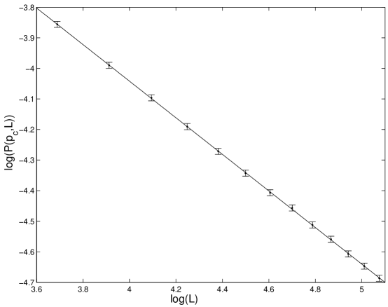
Figure 4: Plot of $\log(P(p_{c},L))$ versus $\log(L)$. The slope of the straight line gives $\frac{\beta}{\nu}=0.60\pm 0.01$

Thus the slopes of these curves should also give $\nu$.
In Fig. 1 we present results of the simulation for the massless harmonic crystal on a cubic lattice with periodic boundary conditions. Each $\Gamma_{L}$ was averaged over $48000$ samples except for $L=160$ where the average is over $2400$ samples. To determine the error bars we have divided the output of the simulations into 10 parts and assuming that the averages are Gaussian distributed we evaluated the variance which we used as a measure of the uncertainty. From the intersection of the curves, after interpolation, we obtain $p_{c}=0.16\pm 0.01$. Comparing the slopes of the $R_{L}$ curves for $L=80$ and $L=40$ we obtain $\nu=2.1\pm 0.5$. From the value of $R_{L}$ at the intersection point of the curves we obtain $\frac{\gamma}{\nu}=1.8\pm 0.1$. We actually computed $\Gamma_{L}$ for the sequences $L=10,20,40,80,160$ and $L=15,30,60,120$. All the simulation results are consistent with what is plotted in Fig. 1 where we have used only part of these simulations since the plot is otherwise cluttered. These values clearly show that our system is in a different universality class from independent percolation since for the latter $\nu=0.876\pm 0.001$ and $\frac{\gamma}{\nu}=2.045\pm 0.001$  [19].
The above method is good for finding the percolation threshold and the ratio of critical exponents $\frac{\gamma}{\nu}$ but clearly does not give good results for $\nu$. To obtain more precise result for the percolation correlation length exponent we evaluated the probability that there is a “wrapping cluster”, i.e. one that wraps around the torus, for different densities $p$ of occupied sites and different linear sizes $L$.
For fixed $L$ we denote by $p_{c}^{eff}$ the value of the density of occupied sites for which one half of the realizations will have such a wrapping cluster. This should obey the following scaling relation $p_{c}^{eff}-p_{c}\sim L^{-\frac{1}{\nu}}$ [1]. For sizes between $30$ and $100$ we evaluated $p_{c}^{eff}$ from doing simulation in a range between $p=0.13$ and $p=0.25$ in steps of $0.005$. For each such system $24000$ samples were generated. The slope of $\log(p_{c}^{eff}-p_{c})$ versus $\log(L)$ should give us $\nu$. A plot of the results is presented in Fig. 2. The slope of the fitted straight line is $0.50\pm 0.01$ which gives $\nu=2.00\pm 0.04$. This is in good agreement with the theoretical prediction $\nu=2$ of Weinrib and Halperin [4].
We have used the obtained values of $p_{c}$, $\frac{\gamma}{\nu}$ and $\nu$ to draw Fig. 3 where we see a good collapse of the data points to a smooth curve.
We also calculated the ratio of the critical exponents $\frac{\beta}{\nu}$. We did this by finding the fraction of sites that belong to the largest cluster in a system of linear size $L$, $\frac{P(p_{c},L)}{L^{d}}$,when we simulate at the approximate critical density. From (7) we see that $\frac{P(p_{c},L)}{L^{d}}\sim L^{-\frac{\beta}{\nu}}$. The result for systems of size from $40$ to $170$ averaged over $24000$ samples is presented in (Fig. 4). From the slope of the fitted straight line we obtain $\frac{\beta}{\nu}=0.60\pm 0.01$. Moreover, the fact that $P(p_{c},L)$ follows well a power law behavior supports our contention that the true critical value is near $p_{c}=0.16\pm 0.01$. Observe also that $2\frac{\beta}{\nu}+\frac{\gamma}{\nu}=3.0\pm 0.2$ and thus the hyper-scaling relation is satisfied.

III The Voter Model

III.1 Formulation

Another system whose pair correlations decays like that of the massless harmonic crystal is the voter model in $\mathbb{Z}^{d}$  [11].
The voter model is defined through a stochastic time evolution. Each lattice site is occupied by a voter who can have two possible opinions, say yes or no. With rate $\tau^{-1}$ the voter at site x adopts the opinion of one of his/her $2d$ neighbors chosen at random. More specifically letting $\rho(x)=0,1$, $x\in\mathbb{Z}^{d}$, the time evolution of the voter model is specified by giving the rate $C_{v}(x,\mathbf{\rho})$ for a change at site x when the configuration is given by $\mathbf{\rho}$

$$C_{v}(x,\mathbf{\rho})=\frac{1}{\tau}\left[1-\frac{1}{2d}(2\rho(x)-1)\sum_{|y-x|=1}(2\rho(y)-1)\right]$$

where $\tau$ sets the unit of time.
It is clear that for the voter model on a finite set $\Lambda\subset\mathbb{Z}^{d}$ with periodic or free boundary conditions (b.c.), there will be only two possible stationary states: either $\rho(x)=1$ or $\rho(x)=0$ for all $x\in\Lambda$. The same is true for the voter model on an infinite lattice in one and two dimensions: the only stationary states are the consensus states. However for $d\geq 3$ there are, as for the massless harmonic crystal, unique stationary states for every density $p$ of positive spins, $p=\left<\rho(x)\right>$. The correlations in this state decay as

$$\left<\rho(x)\rho(y)\right>-p^{2}=p(1-p)G_{d}(x-y)$$

where $G_{d}(x)$ is the probability for a random walker, starting at $x\in Z^{d}$ to hit the origin before escaping to infinity. It is well known that $G_{d}(x)\sim\frac{1}{|x|^{d-2}}$ for $d\geq 3$, i.e the pair correlation for the voter model has the same long range behavior as the massless harmonic crystal.

III.2 Simulation Method

An efficient method to simulate the voter model is to consider a box $B_{\mathcal{L}}$ of linear size ${\mathcal{L}}$ with stochastic boundary conditions, i.e. when a voter looks at the boundary he sees $1$ with probability $p$ and $0$ with probability $1-p$. It is then possible to show that the distribution of the configuration of voters in a box $B_{L}$ of size $L<\mathcal{L}$ centered inside $B_{\mathcal{L}}$ and far away from the boundary will approach the steady state measure (restricted to $B_{L}$) with density p for the voter model when $\mathcal{L}\rightarrow\infty$. In order to sample from the measure for the voter model inside $B_{\mathcal{L}}$ with such stochastic boundary conditions we use the following algorithm: Start a random walk from each site of $B_{L}$ and let these random walks move independently until two of them meet in which case they coalesce. When a random walk hits the boundary of $B_{\mathcal{L}}$ it is frozen. We continue this until all the random walkers either coalesce or are frozen. After this is done we independently for each frozen walker, assign the value $1$ with probability $p$ and the value $0$ with probability $1-p$, then assign that same value to its ancestors, that is all the random walkers that have coalesced with it. In this way we assign values 1 or zero to all the sites in $B_{L}$. One can prove that in this way we sample configurations inside $B_{L}$ with the distribution coming from the voter model in $B_{\cal{L}}$ with the stochastic boundary conditions discussed above. The advantage of this way of simulating is that one is guaranteed that the sampling is from the steady state measure with these boundary conditions.

III.3 Results

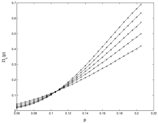
Figure 5: Plot of $\Pi_{L}$ versus p for the $d=3$ voter model. We have plotted data points for $L=10,15,20,25$ and $30$ from $p=0.06$ to $p=0.205$ in steps of $0.005$. Each point is an average over $10^{5}$ samples. The error bars are not shown since on this scale they are too small.

Using this method of generating configurations inside $B_{L}$ for different p we looked for a spanning cluster inside $B_{L}$. We did simulations for sizes $L=10,15,20,25$ and $30$ with $\mathcal{L}=160$. The results which are the same for all $\mathcal{L}$ in the range $(120,160)$ are presented in Fig. 5. If we assume the scaling form for the spanning probability  [1]

$$\Pi_{L}(p)=F((p-p_{c})L^{1/\nu})$$ (9)

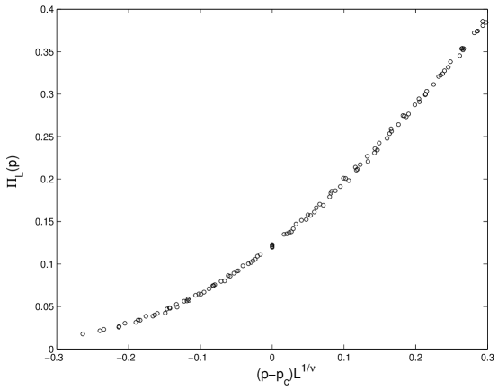
Figure 6: Plot of $\Pi_{L}$ versus $(p-p_{c})L^{\frac{1}{\nu}}$ for the $d=3$ voter model for $p_{c}=0.105$ and $\nu=2$. We have used the same data that was used to create Fig. 5

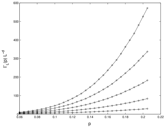
Figure 7: Plot of $\Gamma_{L}L^{-d}$ versus $p$ for the $d=3$ voter model. We have plotted data points for $L=10,15,20,25$ and $30$ from $p=0.06$ to $p=0.205$ in steps of $0.005$. Each point is an average over $10^{5}$ samples. The error bars are not shown since on this scale they are too small.

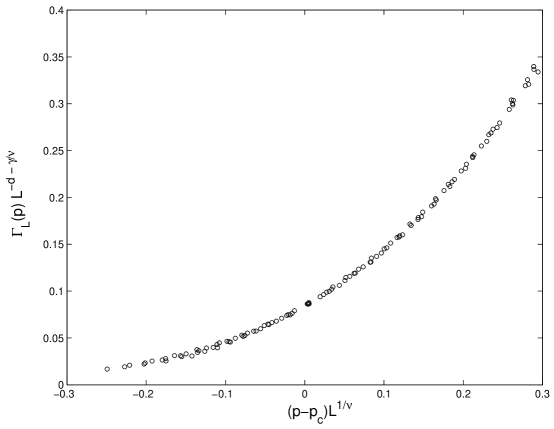
Figure 8: Plot of $\Gamma_{L}L^{-d-\frac{\gamma}{\nu}}$ versus $(p-p_{c})L^{\frac{1}{\nu}}$ for the $d=3$ voter model for $p_{c}=0.105$, $\nu=2$ and $\frac{\gamma}{\nu}=1.9$. We have used the same data that was used to create Fig. 7

then by collapsing the data Fig. 6 we obtain $p_{c}=0.10\pm 0.01$ and $\nu=2\pm 0.2$.
To find $\frac{\gamma}{\nu}$ we measured $\frac{\Gamma_{L}}{L^{3}}$ and we assume the scaling form (5). Note that in this case we do not have periodic boundary conditions. Results from the simulation are presented in Fig. 7. Collapsing the data Fig. 8 we obtain $p_{c}=0.10\pm 0.01$, $\frac{\gamma}{\nu}=1.9\pm 0.2$ and $\nu=2\pm 0.2$.
Analogous simulation measurements for $P(p,L)$ gave $\frac{\beta}{\nu}=0.6\pm 0.1$. As in the case of the massless harmonic crystal the exponents we found satisfy the hyper-scaling relation $2\frac{\beta}{\nu}+\frac{\gamma}{\nu}=d$. The exponents for both the massless harmonic crystal and voter model seem to agree within the error bars.

III.4 Comparison of $p_{c}$ with previous simulations

The percolation transition in the $d=3$ voter model was first investigated in [13]. This was done by considering voters who occasionally change their opinions spontaneously, i.e. independently of what their neighbors are doing. They do this with probability $\lambda$. In terms of flip rates one has

$$C(x,\rho)=(1-\lambda)C_{v}(x,\rho)+\frac{\lambda}{\tau}\left[1+(1-2p)(2\rho(x)-1)\right],$$

where $0\leq p\leq 1$ and $0\leq\lambda\leq 1$ and $C_{v}$ is the voter model flip rates. This leads to a stationary state in any periodic box of size $L^{d}$ with density of pluses equal to $p$. As $\lambda$ increases from 0 to 1 we go from the voter model to an independent flip model. The stationary state of the latter is a product measure with density $p$. This model was studied rigorously in  [20] where it was named the noisy voter model.
In [13] the authors used (5), on simulation results of the noisy voter model on lattices with periodic boundary conditions, to obtain $p_{c}(\lambda)$ for $\lambda>0.1$. For $d=3$ they found by extrapolation $p_{c}(\lambda)\sim 0.16$ as $\lambda\rightarrow 0$.
We have repeated the simulations in  [13] for larger lattice sizes and smaller values of $\lambda$. We simulated systems with $\lambda$ as small as 0.01 each with 24000 “effectively uncorrelated” samples and sizes up to $80$. From our results we can extrapolate $p_{c}(\lambda)\rightarrow 0.15$ as $\lambda\rightarrow 0$, a value slightly lower than the result in  [13]. We also observed that, as expected, the critical exponents for the noisy voter model agree, for the given range of $\lambda$, with the critical exponents of independent percolation.
This leaves a significant difference with the result for $p_{c}$ obtained in the previous section. We believe that the answer lies in the necessary extrapolation to $\lambda=0$. Since the autocorrelation time grows exponentially with lambda, this means we have to wait for more and more Monte Carlo steps to get independent samples. To check this explanation we investigated the percolation transition in the harmonic crystal with a mass M. This mass acts much like the random flips in the voter model. For both models the pair correlation decays exponentially. In the harmonic crystal the characteristic length scale is $\xi_{M}=\frac{1}{M}$. An easy calculation shows that the characteristic length scale for the noisy voter model is $\xi_{\lambda}=\sqrt{\frac{1-\lambda}{6\lambda}}$. The noisy voter model with the smallest lambda that we simulated , $\lambda=0.01$, thus corresponds to $\xi_{\lambda}$ roughly equal to 4 (unit distance is the lattice spacing). In the language of the massive harmonic crystal this corresponds to $M\sim 0.25$. Estimating the percolation threshold of the massless harmonic crystal by the extrapolation method we used for the voter model using $M\geq 0.25$ yields a $p_{c}(M)\sim 0.21$ when $M\rightarrow 0$. This is obviously a large overestimate of $p_{c}=0.16$ which was obtained by directly simulating the massless harmonic crystal. This shows that the extrapolation method greatly overestimates the true $p_{c}$.

IV Concluding Remarks

We have performed Monte Carlo simulations to obtain the critical percolation density and some critical exponents for the massless harmonic crystal and the voter model in $\mathbb{Z}^{3}$. We found, for the first time a value of $p_{c}$ for the former and using a novel method of simulation for the voter model found a new more reliable value of $p_{c}$ for this system. The critical exponents for both models agree within the error bars. This suggests that both percolation models are in the same universality class and confirms the theoretical predictions made in  [4]. The result for the correlation length critical exponent $\nu=2$ supports the conjecture by WH that the relation $\nu=\frac{2}{a}$ is exact.
It is believed that not only the critical exponents but also the finite size scaling functions are universal. While this is certainly consistent with our simulations we have not checked this carefully. Such a check would require measuring quantities for the two systems in the same way. This is not what we have done here as we wanted to use the most efficient method for each system.
We mention here that there has been much activity in generalizing the voter model in various ways  [21]. Based on our present work we expect that the nature of the percolation transition in these models will depend only on the asymptotic behavior of $G(r)$. We have however not investigated this. Our simulation method may be extendable to some of these systems.
The reported simulations were done on a Sun Microsystems HPC-10000 system.

References

- [1] D.Stauffer and A.Aharony, Introduction to Percolation Theory, 2nd ed. (Taylor Francis, New York, 1994).
- [2] G.Grimmet, Percolation, 2nd ed. (Springer-Verlag, Berlin, 1999).
- [3] S. Smirnov, C. R. Acad. Sci. Paris 333, 239 (2001).
- [4] A. Weinrib and B. Halperin, Phys. Rev. B 27, 413 (1983).
- [5] D. Bernard, G. Boffetta, A. Celani and G. Falkovich, Nature Physics 2, 124 (2006).
- [6] T. Abete, A. de Candia, D. Lairez and A. Coniglio, Phys. Rev. Lett. 93, 228301 (2004).
- [7] A. Weinrib, Phys. Rev. B 29, 387 (1984).
- [8] S. Prakash, S. Havlin, M. Schwartz, and H.E. Stanley, Phys. Rev. A 46, R1724 (1992).
- [9] J.Bricmont, J. Lebowitz, and C.Maes, Jour. Stat. Phys. 48, 1249 (1987).
- [10] G. Giacomin (private communication).
- [11] T.M. Liggett, Interacting Particle Systems (Springer-Verlag, New York, 1985).
- [12] L. Chayes, J. Lebowitz and V. Marinov (in preparation).
- [13] J. Lebowitz and H. Saleur, Physica A 138, 194 (1985).
- [14] H.-O. Georgii, Gibbs measures and phase transitions, de Gruyter Studies in Mathematics 9 (Walter de Gruyter & Co., Berlin, 1988)
- [15] A. van Enter, R. Fernandez, and A. Sokal, Jour. Stat. Phys 72, 879 (1993).
- [16] S. Sheffield, Gaussian free fields for matematicians, arXiv: math.PR/0312099.
- [17] H. Saleur and B. Derrida, J. Physique 46, 1043 (1985).
- [18] K. Binder and D.W. Heermann, Monte Carlo Simulation in Statistical Physics:an introduction (Springer-Verlag, Berlin, 1992).
- [19] H.G.Ballesteros, L.A. Fernandez, V. Martin-Mayor, A. Munoz Sudupe, G. Parisi, and J.J. Ruiz-Lorenzo, J. Phys. A 32, 1 (1999).
- [20] B. Granovsky and N. Madras, Stoch. Proc. Appl. 55, 23 (1995).
- [21] I. Dornic, H. Chate, J. Chave and H. Hinrichsen, Phys. Rev. Lett. 87, 045701 (2001).