The Influence of Interatomic Bonding Potentials on Detonation Properties

Abstract

The dependence of macroscopic detonation properties of a two-dimensional diatomic (AB) molecular system on the fundamental properties of the molecule were investigated. This includes examining the detonation velocity, reaction zone thickness, and critical width as a function of the exothermicity ($Q$) of the gas-phase reaction ($\textrm{AB}\rightarrow(1/2)(\textrm{A}_{2}+\textrm{B}_{2})$) and the gas-phase dissociation energy ($D_{e}^{\textrm{AB}}$) for $\textrm{AB}\rightarrow\textrm{A}+\textrm{B}$. Following previous work, molecular dynamics (MD) simulations with a reactive empirical bond-order (REBO) potential were used to characterize the shock-induced response of a diatomic AB molecular solid, which exothermically reacts to produce $\textrm{A}_{2}$ and $\textrm{B}_{2}$ gaseous products. Non-equilibrium MD simulations reveal that there is a linear dependence between the square of the detonation velocity and each of these molecular parameters. The detonation velocities were shown to be consistent with the Chapman-Jouguet (CJ) model, demonstrating that these dependencies arise from how the Equation of State (EOS) of the products and reactants are affected. Equilibrium MD simulations on microcanonical ensembles were used to determine the CJ states for varying $Q$s and radial distribution functions to characterize the atomic structure. The character of this material near the CJ conditions was found to be rather unusual consisting of polyatomic clusters rather than discrete molecular species. It was also found that there was a minimum value of $Q$ and a maximum value of $D_{e}^{\textrm{AB}}$ for which a pseudo-one dimensional detonation could not be sustained. The reaction zone of this material was characterized under both equilibrium (CJ) and transient (underdriven) conditions. The basic structure is consistent with the Zeldovich- von Neumann-Döring model with a sharp shock rise and a reaction zone that extends to 200-300 Å. The underdriven systems show a build-up process which requires an extensive time to approach equilibrium conditions. The rate stick failure diameter (critical width in 2D) was also found to depend on $Q$ and $D_{e}^{\textrm{AB}}$. The dependence on $Q$ could be explained in terms of the reaction zone properties.

I Introduction

The simplest theory of detonation is that of Chapman and Jouguet (CJ) Fickett and Davis (1979); Mader (1979); Davis (1987). In this one dimensional theory the shock rise and reaction are treated as instantaneous. On a pressure-specific volume ($P$-$v$) state diagram the point of tangency between a Rayleigh line (an expression of the conservations of mass and momentum across the detonation front traveling at a given velocity) and a Hugoniot (conservation of energy) is the CJ state. The slope of the Rayleigh line is proportional to the negative of the square of the product of the initial density ($\rho_{0}$) of the material and the detonation velocity ($u_{s}$). If $u_{s}$ is any slower than the CJ value ($u_{sj}$), the Rayleigh line does not intersect the Hugoniot, and there is no solution to the conservation equations. In this light the CJ state is determined by the Equation of State (EOS) of the products and the initial state of the reactants, and that determines the minimum detonation velocity ($=u_{sj}$) for the system. This hypothesis predicts the detonation properties of high performance high explosives (HE) reasonably well despite its crude assumption Fickett and Davis (1979); Mader (1979),

A more detailed model is the classical theory of detonation due to Zeldovich Zeldovich (1960), von Neumann von Neumann (1942), and Döring Doering (1943) (ZND) which, following the initial shock compression, allows the molecules of a high explosive (HE) to react and expand. This is represented by a pressure profile, whose principal features are (1) an instantaneous shock rise to a state where the reactants are heated and compressed, and this is typically referred to as the von Neumann (VN) spike; (2) a fixed-width reaction zone, in which reactions provide the chemical energy to maintain the detonation wave as density and pressure decrease; and (3) a Taylor wave of the rarefying product gases. In the case where the detonation is supported by a driving piston, there will be a constant state in the pressure profile from some point behind the reaction zone back to the piston. If the piston is driven at the particle velocity of the unsupported final state (matching the CJ state at the end of the reaction zone), there will be no Taylor wave, and only the reaction zone will be observed. If the piston is driven at a greater velocity than this critical value, then the detonation velocity will be increased. The detonation is now said to be overdriven, and the flow in the constant zone is subsonic in the frame of the detonation front. For the case where the detonation is underdriven with respect to the CJ conditions, it should asymptote to the minimum detonation velocity determined by the CJ state, and only the Taylor expansion will be affected by a disturbance behind the final state Fickett and Davis (1979).

Molecular Dynamics (MD) simulations are well suited to test these and other aspects of detonation theory and their associated models under controlled microscopic conditions as demonstrated by work going back over a decade Brenner et al. (1993); White et al. (2000); Rice et al. (1996a, b); White et al. (2001); Maffre and Peyrard (1992); Erpenbeck (1992); Robertson et al. (1991); Haskins and Cook (1994); Haskins et al. (1998); Germann et al. (2002); Holian et al. (2002); Maillet et al. (2004). With MD it is possible to control the inherent material properties, initial material state, and confinement conditions of the simulation. For example, using a predissociative Morse potential, Maffre et al. performed a preliminary study of “hot spots”, which arise at heterogeneities. Maffre and Peyrard (1992). Similar work was also done using voids and gaps as the heterogeneities Germann et al. (2002); Holian et al. (2002). Monte Carlo techniques have been incorporated with MD to find thermodynamic properties and the Hugoniot of a system of hard spheres Erpenbeck (1992) and, more recently, a reactive model close to the one used here Rice et al. (1996a). Tests of the dependence of the critical flyer plate velocity needed to initiate detonation on the flyer plate thickness Haskins and Cook (1994) have been studied. Rice et al. have characterized some aspects of the reaction mechanism Rice et al. (1996b) and demonstrated correspondence to hydrodynamic theory for a model system Rice et al. (1996a). Attempts have been made to connect the micro- and macroscales with MD and hydrodynamic codes Maillet et al. (2004).

Several of these simulations Brenner et al. (1993); White et al. (2000); Rice et al. (1996a, b); White et al. (2001); Robertson et al. (1991); Haskins and Cook (1994); Haskins et al. (1998); Germann et al. (2002); Holian et al. (2002); Maillet et al. (2004) have been conducted in two dimensions using a Reactive Empirical Bond Order (REBO) potential Brenner et al. (1993), representing a simple material composed of two atom types (A and B). REBO is a modification of Tersoff’s Empirical Bond Order (EBO) potential Tersoff (1986). The restriction to two dimensions allows significantly greater spatial and time scales to be accessed for given computational resources, though three dimensional simulations have also been pursued. The process of shock-induced reversible chemical reactivity, converting reactant AB molecules exothermically into $\textrm{A}_{2}$ and $\textrm{B}_{2}$ products, is represented in the AB model of Brenner et al. Brenner et al. (1993). With this, it has been demonstrated that non-equlilibrium MD (NEMD) simulations using REBO potentials produce detonations consistent with continuum theory and experimental observations White et al. (2001). However, most of these prior studies with REBO have focused on using a single set of materials characteristics and energetic parameters. It has been found that seemingly subtle variations in the model or parameters can result in rather dramatic changes in behavior. Also, because of computational requirements, the simulations have been limited in scale such that significant features are not always resolved. Utilizing large-scale simulations done with the SPaSM parallel MD code Lomdahl et al. (1993), our aim is to extend the work of Haskins et al. Haskins et al. (1998) by investigating the dependencies of the detonation velocity, the reaction zone thickness, and the critical width that a HE must have in the transverse directions to sustain detonation on these atomistic energetics. This will be done with controlled variations in the fundamental microscopic energetic quantities, namely the exothermicity ($Q$) of the reaction and AB dissociation energy ($D_{e}^{\textrm{AB}}$), in order to document more thoroughly the relationship between microscopic properties and macroscopic behavior.

This paper is organized as follows. In Sec. II we lay out the details of the potential and the simulations used. In Sec. III, using equilibrium microcanonical (NVE) ensembles, we map out the product Hugoniot for set values of parameters and compare the expected CJ velocities of the detonation fronts to those found by unsupported NEMD simulations. The CJ states of these materials are also characterized here.

In Sec. IV we study the relationship of $Q$ to the equation of state (EOS) in order to better understand the results from Sec. III. In Sec. V we characterize the width of the reaction zone and compare this to the critical minimum width ($W_{c}$) which a 2D sample must have in the direction normal to detonation front’s propagation in order for that detonation to be sustained. (In 3D cylindrical samples, of course, the critical width analog is known as the failure diameter, and the experimental setup is called a rate stick.)

II Methods

There are several versions of REBO used in the related literature. The version used here is due to Brenner et al. Brenner et al. (1993). In it the binding energy of an N-atom system takes the form,

$$E_{b}=\sum_{i}^{N}\sum_{j>i}^{N}\{f_{c}(r_{ij})[V_{R}(r_{ij})-\overline{B}_{ij}V_{A}(r_{ij})]+V_{\textrm{vdW}}(r_{ij})\},$$ (1)

where $r_{ij}$ is the distance from atom $i$ to atom $j$. $V_{\textrm{A}}$ and $V_{\textrm{R}}$ are the attractive and repulsive terms, respectively, of a Morse intramolecular potential $V_{\textrm{A}}-V_{\textrm{R}}$, and $\overline{B}_{ij}\equiv(B_{ij}+B_{ji})/2$, which contains the effective valence and is designed to create dimers. Depending on the local environment, $\overline{B}_{ij}$ varies from 0 to 1. If atom $i$ has no neighbors (defined by $f_{c}(r)$) other than $j$, $B_{ij}=1$ and the full Morse attraction is felt. On the other hand, if $i$ has two neighbors, $j$ and $k$, and $r_{ij}<r_{ik}$, $0<B_{ik}<B_{ij}<1$, i.e., the $ij$ and $ik$ attractions are both reduced, but more so for the pair farther apart $(ik)$ than for the nearer pair $(ij)$. The effect of this is to introduce a preferential valence of one for each atom. A weak intermolecular van der Waals (Lennard-Jones form) interaction $V_{\textrm{vdW}}$ stabilizes a crystalline AB molecular solid, at least at low temperatures. $f_{c}$ is a cutoff function which smoothly takes the potential to zero within a finite distance. The rest of the precise functional forms and parameters are contained in the errata of Brenner et al. (1993).

Isolated XY molecules (X,Y $\in$ {A,B}) have binding energies $D_{e}^{\textrm{XY}}$ (since $\overline{B}_{ij}=1$); these are the fundamental parameters which we will vary from their baseline values Brenner et al. (1993), $D_{e}^{\textrm{AA}}=D_{e}^{\textrm{BB}}=5.0$ eV and $D_{e}^{\textrm{AB}}=2.0$ eV. These two parameters (constraining $D_{e}^{\textrm{AA}}=D_{e}^{\textrm{BB}}$) are related to the exothermicity ($Q$) through:

$$\textrm{2AB}\rightarrow\textrm{A}_{2}+\textrm{B}_{2}+2Q$$ (2a)

$$Q=D_{e}^{\textrm{AA}}-D_{e}^{\textrm{AB}}.$$ (2b)

$D_{e}^{\textrm{AB}}$ is just the energy required to dissociate an isolated AB molecule:

$$\textrm{AB}+D_{e}^{\textrm{AB}}\rightarrow\textrm{A}+\textrm{B}.$$ (3)

$Q$ is varied from 1.5 eV to 10.0 eV by holding $D_{e}^{\textrm{AB}}$ constant at 2.0 eV while $D_{e}^{\textrm{AA}}$ is varied from 3.5 eV to 12.0 eV. $D_{e}^{\textrm{AB}}$ is varied from 0.5 to 3.5 eV, by varying $D_{e}^{\textrm{AB}}$ and $D_{e}^{\textrm{AA}}$ together so that their difference, $Q$, is constant at 3.0 eV.

In each NEMD setup a stable A₂ flyer plate, four cells thick (two A₂ dimers per cell), impacts a 2D metastable AB herringbone lattice at $z=0$ and a velocity of 9.8227 km/s (Fig. 1). The sample has an initial temperature of 11.6 K. (The potential parameters roughly correspond to $\textrm{N}_{2}$, with a correspondingly low melting and boiling point.) The resulting unsupported shock travels to the right, $\hat{z}>0$. In $\hat{z}$ the boundaries are culled, i.e., particles are lost when they exit the simulation cell. In the lateral $\hat{x}$ direction the boundaries are periodic in Sec. III to study planar detonations or culled, but padded with free space, in Sec. V to determine failure widths. In computations involving the reaction zone thickness and detonation velocity, the sample initially is at least 48 lattice cells in $\hat{x}$ and 600 in $\hat{z}$. The simulation is allowed to run for at least 30.54 ps with a timestep $dt=0.25$ fs. The minimum duration is the same for trials determining $W_{c}$ versus  either $Q$ or $D_{e}^{\textrm{AB}}$. The maximum length in cells for these calculations is 360 cells in $\hat{z}$. In the equilibrium MD calculations presented in Sec. IV, the samples are $25\times 25$ $\textrm{cells}^{2}$ with periodic boundary conditions. The simulations are run for 40 ps with measurements averaged over the last 30 ps.

(a)
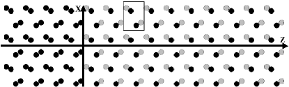
(b)

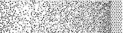
Figure 1: (a) A snapshot of a magnified section of the initial sample in a flyer driven unsupported NEMD simulation of detonation at $t=0$. The A atoms are black and the B gray. The A₂ flyer plate can be seen to the left of the x axis. The box encloses a herringbone lattice cell, consisting of 2 AB dimers.
(b) A snapshot of the detonating sample with the detonation front moving toward the right.

III Detonation Velocity and the CJ conditions

Haskins et al. report a linear dependence of $u_{s}^{2}$ on $Q$ for a similar AB material Haskins et al. (1998). We repeat this study with a slightly different REBO potential and further it by varying the AB dissociation energy ($D_{e}^{\textrm{AB}}$). One expects the velocity to increase with $Q$ because the increased exothermicity of the reaction increases the temperature and pressure of the products. Fig. 2 confirms the linear relationship between $u_{s}^{2}$ and $Q$ for this particular system. The differences between values in Fig. 2 and Haskins et al. (1998) are due to differences in other REBO parameters and the flyer’s thickness and impact velocity. Here, impact velocity is not raised above 9.8227 km/s in order to avoid the “fast detonation regime” Maffre and Peyrard (1992) (which may have been an artifact of the model used there). At values of $Q<1.5$ eV, the linear relationship begins to fail, and the system would not sustain a propagating detonation for $Q=1.3$ eV. This failure point likely arises because the reaction rate (determined by the temperature at the initial shock front) has become sufficiently slow such that it does not approach completion within the subsonic region of the reaction zone Fickett and Davis (1979). The temperature at the shock front can be estimated from the kinetic energy of the shock front, given by the right-hand axis labels in Figure 2.

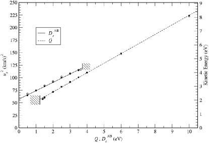
Figure 2: Square of the detonation velocity ($u_{s}^{2}$) vs. AB dissociation energy ($D_{e}^{\textrm{AB}}$) and exothermicity ($Q$). The flyer thickness and impact velocity are held fixed, so detonation is not sustained in regions where it is reported to in Haskins et al. (1998). Failure is indicated by the shaded boxes. A sustained detonation is defined as not failing before the right edge of the sample. Error bars are smaller than the size of the symbols. The scale on the right gives the kinetic energy of an atom traveling at $u_{s}$. The filled symbols are from NEMD simulations with a free boundary at $z=0$. The empty symbols are from NEMD simulations with a momentum mirror at $z=0$. The linear fits are $u_{s}^{2}=33.205+19.137Q$ and $u_{s}^{2}=57.251+16.694D_{e}^{\textrm{AB}}$.

The dependence of $u_{s}^{2}$ on $D_{e}^{\textrm{AB}}$ is also found to be linear and increasing (Fig. 2). Our initial expectation was that the variations in $D_{e}^{\textrm{AB}}$ would primarily affect the activation energy of the reaction and could quench the detonation when the activation energy became too great to be readily overcome at the temperature of the initial shock state. The failure to maintain a propagating detonation for $D_{e}^{\textrm{AB}}>3.7$ eV is possibly a manifestation of this. The strong dependence of $u_{s}^{2}$ on $D_{e}^{\textrm{AB}}$ indicates that other aspects of the system are likely being affected by this perturbation.

To understand these relationships more thoroughly, we turn first to the basic test of standard detonation theory, which is to compare predictions based on the CJ state determined from equilibrium MD simulations with the evaluation of detonation propagation from NEMD studies. The theoretical CJ state for a 1D detonation is at a sonic point at thermochemical equilibrium Fickett and Davis (1979). If this is an improper assumption and the reaction is incomplete at the arrival time of the sonic point, it could account for a discrepancy between the theoretical and actual detonation velocities. For a slightly different REBO potential, Rice et al. found a detonation velocity from an unsupported simulation that was 6.1% lower than that found from the calculation of their CJ state Rice et al. (1996a).

Our procedure for locating the CJ state is described here and similar to that of Rice et al. Rice et al. (1996a). At different values of specific volume ($v$), sets of microcanonical (NVE) MD simulations of 2500 particles are run for 40 ps, providing sufficient time to equilibrate. The onset of equilibrium is determined by the shape of the time evolution of the average properties of simulation. After each of these reaches a plateau, as determined by visual inspection, the simulation is allowed to continue. A runs-above-the-median test is performed to determine that the curves are flat with only random fluctuations. At each value of $v$, the value of specific internal energy ($E$) is sought that is a solution of the Hugoniot jump condition,

$$\frac{1}{2}(v_{0}-v)P=E-E_{0}$$ (4)

(energy conservation in which $P_{0}=0$), where $P=\frac{1}{2}(P_{zz}+P_{xx})$ is the hydrostatic pressure, $P_{\alpha\beta}$ is the negative of the corresponding component of the stress tensor and has ideal and virial components, and the subscript 0 indicates the state in front of the detonation front. Once $\langle E\rangle$ is determined for the present value of $v$, NVE ensemble averages $\langle x\rangle$ of other thermodynamic quantities are computed by linear interpolation.

By repeating this procedure for several values of $v$, the product $P$-$v$ Hugoniot is determined (Fig. 3). Using the remaining jump conditions, mass conservation:

$$u_{p}/u_{s}=(v_{0}-v)/v_{0}$$ (5)

and momentum conservation in which $P_{0}=0$,

$$u_{s}u_{p}=v_{0}P,$$ (6)

one can find $u_{s}$ as a function of the particle velocity at the final state ($u_{p}$). The minimum possible value of $u_{s}$ is the CJ value Fickett and Davis (1979), so the minimum of $u_{s}$ versus any thermodynamic parameter is at the CJ value of that parameter (e.g., see Fig. 4). We use the minimum determined by these means as iterative approximations of the CJ state (see Table 1 under the CJ-Interpolation column). We refine the process by fitting a quadratic through the points surrounding the minimum. We must be careful to include a domain small enough that a quadratic is a good approximation to the data, yet large enough to include more than three data points in order to get a proper estimate of the error from the goodness-of-fit parameter.

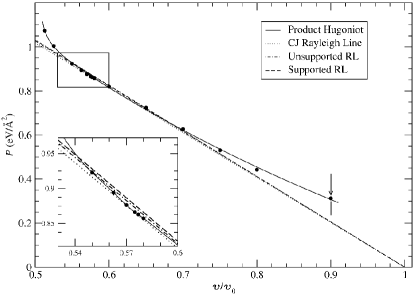
Figure 3: A $P$-$v$ state diagram of the equilibrium product Hugoniot. The solid curve is a guide to the eye. The dotted/dashed curves are Rayleigh lines plotted using the initial state ($P_{0}=0.0,v/v_{0}=1.0$) and a slope of -$u_{s}^{2}\rho_{0}$, where $\rho$ is the mass density and $u_{s}$ for each curve, from the steepest down, is the median value of shock velocity taken from the supported detonation, the EOS calculation, and the unsupported detonation. The arrows represent a series of simulations at constant $v$ used to find the datum to which they point. The box is a magnification.

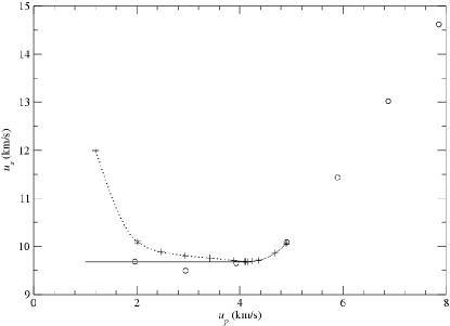
Figure 4: Shock velocity ($u_{s}$) vs. particle velocity ($u_{p}$). Similar plots can be made for other thermodynamic variables on the abscissa. Each point corresponds to a different value of specific volume ($v$), which increases along the abscissa in the direction opposite that of $u_{p}$. A constant line is drawn at the determined minimum value of $u_{s}$. The dotted part of the curve indicates that which is not dynamically accessible. Instead NEMD simulations with pistons moving at $u_{p}$ less than the value at which the minimum is located ideally should follow the constant line. The open circles show the results of piston driven NEMD simulations where the piston is driven at $u_{p}$.

Table 1: Values measured or defined in a process which determines the CJ state through a series of microcanonical equilibrium simulations or in the constant zone of a non-equlilibrium simulation of a critically supported detonation (Sec. IV). $v$ is the specific volume. $u_{s}$ is the shock velocity. $u_{p}$ is the particle velocity at the final state. $T$ is the absolute temperature. $U$ is the potential energy. $E$ is the specific internal energy, and $P$ is the 2D pressure. Values marked with asterisks are input into the corresponding simulation(s). The parentheses indicate the error in the last two digits of the corresponding reported value.

	CJ Interpolation			Supported NEMD
$Q$ (eV)	1.5*	3.0*	6.0*	3.0*
$v/v_{0}$	0.50182(24)	0.57164(81)	0.6171(19)	0.5747(16)
$u_{s}$ (km/s)	8.0720(11)	9.6758(90)	12.2055(20)	9.7360(40)
$u_{p}$ (km/s)	4.0212(13)	4.1446(40)	4.673(22)	4.144*
$\langle k_{B}T\rangle$ (eV)	0.4017(14)	0.7839(43)	1.7550(90)	0.7791(56)
$\langle U\rangle$ (eV)	-0.25156(79)	-0.5605(21)	-1.19657(90)	-0.5746(72)
$\langle E\rangle$ (eV)	0.15012(65)	0.2234(22)	0.5584(84)	0.2234306(15)
$P$ (eV/Å2)	0.70591(33)	0.8726(13)	1.2411(62)	0.8541(83)

To test the CJ results found from these NVE simulations, we run a supported detonation simulation in which an infinitely massive driving piston impacts the AB sample at the CJ-determined velocity ($u_{pj}$). This should establish a constant zone behind the front that should be at the CJ state, with the front propagating at the CJ conditions. Measurements are taken from this run and can be found in Table 1 under the Supported-NEMD column. From Table 1 one can see that many of the values fall within error of one another, although there are some slight discrepancies. It should be noted that the supported-NEMD simulations can include transients from the initiation and/or build-up processes Mader (1979), and these will be explored further below. Still, this discrepancy of 0.35% difference from the unsupported detonation of $u_{s}=9.70961\pm 0.00054$ km/s is quite small, especially since previous evaluations of this same system gave larger discrepancies (9.3 km/s in Brenner et al. (1993) and 9.5 km/s in White et al. (2000)). This is also less of an error than Rice et al. found for their variation.

We repeated several of the tasks performed on $Q$ = 3.0 eV for several more values of $Q$. In Fig. 5 the equilibrium $P$-$v$ Hugoniots for several values of $Q$ are shown. Notice for $Q$ = 6.0 eV that the curve has a nice hyperbolic shape, for which the CJ state for this $Q$ is easy to determine. From it, as was done above, we find $u_{sj}$ to be $12.20552\pm 0.0020$ km/s. The unsupported NEMD simulation with the free boundary gives $12.2031\pm 0.0017$ km/s, a difference that is smaller than the error bars. As $Q$ decreases, the equilibrium Hugoniots flatten out, and it becomes more difficult to identify the exact point of tangency. At $Q$ = 2.0 eV the Hugoniot is well represented by a linear fit. The Hugoniot for $Q$ = 1.5 eV has a negative curvature (convex) section indicating the presence of some sort of phase transition (Fig. 5). It should be noted that $Q$ = 1.5 eV is close to $Q_{c}$, the value for which a detonation can not be sustained.

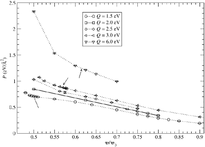
Figure 5: Equilibrium Hugoniots for several values of $Q$. The CJ state is determined for the cases in which $Q$ = 6.0, 3.0, and 1.5 eV. The curve for $Q=2.0$ eV is well fit by a straight line of the form $P=1.69(1-v/v_{0})$. The dotted lines are all guides to the eye. As $Q$ decreases, the Hugoniots go from positive curvature to a zero curvature for $Q=2.0$. The curve for $Q=1.5$ eV contains a section of negative curvature, indicating a phase transition. The arrows point to the determined CJ states.

A comparison of the predicted and measured values of $u_{s}$ for different values of $Q$ are given Table 2. It is found that there is very good agreement between these values, with no discernible discrepancy for $Q$ = 6.0 eV, and only a moderate discrepancy of 2% for $Q$ = 1.5 eV which is very near the failure point. The latter point supports the idea that failure is occurring because of inadequate completion of the reaction when the sonic point passes. Overall though, it can be concluded that these systems are responding in accord with the simple predictions of the Chapman-Jouguet hypothesis. The variations in $u_{s}$ with the molecular parameters is therefore determined by how these effect the Equation of State (EOS) of the products. These aspects will now be examined in further detail.

Table 2: As $Q$ is increased, the predicted ($u_{sj}$) and measured values ($u_{s}$) of the detonation velocity agree more. It is hypothesized that the increased exothermicity causes the reaction to come closer to completion by the sonic point.

$Q$ (eV)	$u_{sj}$ (km/s)	$u_{s}$ unsupported	% difference
1.5	8.0720(11)	7.913(16)	$\approx 2.0$
3.0	9.6758(90)	9.70961(54)	$\approx 0.35$
6.0	12.2055(20)	12.2032(17)	$\approx 0.0$

The curves in Figs. 3 and 4 are rather unusual. For a material behaving like an ideal gas, the former would be expected to have a hyperbolic shape and for the latter a parabolic shape. Here, for large $Q$ (= 6 eV) the resulting curves do have that type of behavior. However, as $Q$ is reduced, the Hugoniot flattens until it eventually gains a convex section, and the $u_{s}$-$u_{p}$ plot evolves into a curve with a double minimum. Therefore we examine the CJ states more closely by simulating a microcanonical ensemble at the determined CJ values of density and internal energy.

A snapshot of the NVE-at-CJ simulation for $Q$ = 3.0 eV is shown in Fig. 6, along with the corresponding radial distribution functions (RDF), $g(r)$, for particles of the same and different type. It is evident from Fig. 6 that, at the CJ state, the system is dominated by short AA and BB contacts, which would be expected for the product species. The interatomic distances for these ($\approx 1.1~{}r_{e}$) is slightly larger than that defined for the isolated molecules ($1.0~{}r_{e}$). By the form of the potential, the introduction of a third particle within the defined bonding distance weakens the attractive part of the potential and moves the minimum of the bonding potential out to greater distances. This aspect is readily explained by the high density at CJ.

What is more intriguing is that there is also a significant number of close A-B interactions at $\approx 1.2~{}r_{e}$, showing that the system has not evolved into a simple mixture of A₂ and B₂. Also, there is a second peak in both RDFs at around $r/r_{e}=2.0$. This second peak indicates that there are clusters of atoms forming at this compression. Looking at the snapshot embedded in Fig. 6, one can see that there appears to be linear oligomers forming.

For comparison Fig. 7 shows the RDF of an NVE simulation of AB at a temperature above its melting point and at the initial density, $v=v_{0}$. It has a strong peak for the AB dimers at $r/r_{e}=1$ as expected. Beyond this, it was expected that there would be a broad peak at  2.8 $r_{e}$, which would be the van der Waals minimum. Although this was observed, somewhat surprisingly, there is a sharp peak just above $r/r_{e}=2$ which is present for all three atomic combinations, as well as another peak at 3 $r_{e}$. The former peak is caused by the positive slope of a section of the inner cutoff spline for the $V_{vdW}$ term, which creates an additional minimum in the multibody potential. Examination of the inset show that the molecules still tend to line up, although the molecules are clearly separate diatomic species. The peak at $r/r_{e}=3$ is probably a result of this alignment and is the distance from a bonded partner of one atom to the non-bonded neighbor which is at  2 $r_{e}$. These features highlight some of the unusual aspects that can arise from these complex interaction potentials.

The notable difference between the RDFs is that the one for the melted AB goes to zero between $r/r_{e}=$ 1.2 and 1.8, which highlights the clear diatomic nature of that system. For the CJ state simulation, there is substantial intensity all across that region, and the RDF value barely drops below 1. Since there are no dissociated atoms or oligomers in the melted AB, it is reasonable that we see a domain above $r/r_{e}=1$ in which a particle will not have a neighbor. Any third particle and its bound partner will be repelled by virtue of the $V_{A}$ term if they approach much closer than 2 $r_{e}$ to a particle in another dimer. At the CJ state density, this repulsion breaks down and clusters of particles form. Similar behavior has also been observed in the systems that Rice et al. studied, where describing the CJ state as one of atomization is a fair description. Rice et al. (1996a, b).

To examine this behavior more closely, we examine the RDFs along the Hugoniot. In particular, we consider the case of $Q=1.5$ eV which has a convex section that indicates a phase transition. The RDFs for several states along that Hugoniot including $v/v_{0}=0.64$, the volume at which the phase transition occurs, are shown in the Fig. 10. For the CJ state, $v/v_{0}=.502$, the RDF is similar to that for the CJ state at $Q=3.0$ eV. The first peak occurs at  1.2 $r_{e}$ with no strong minimums occurring at longer distances. At $v/v_{0}=0.64$, a deep minimum develops at $\approx 1.5~{}r_{e}$ along with peaks at $r/r_{e}=2.0$ and 3.0. From the snapshot at $v/v_{0}=0.64$ (See inset.), one may be convinced that both distinct dimers and extended oligomers are present. At $v/v_{0}=0.75$, the peak sharpening and minimum development are more distinct, and the profile is more reminiscent of the AB melt illustrated in Fig. 7.

To investigate the cause of these clusters, we plot potential energy surfaces (PES) for the interatomic distances of three inline particles as Rice et al. Rice et al. (1996b) did for a different version of REBO. From Fig. 8, which represents an A-A-A configuration, one can see that, at a distance of about 1.35 Å, there is a minimum that allows for trimer formation. This configuration does not exhaust the possible configurations that may occur during reaction because it is constrained to be a linear conformation. The interaction with neighboring atoms, particularly at CJ-type conditions, is also ignored and this could alter the absolute value of the activation energy ($E_{a}$) significantly. However, as Table 3 suggests, $E_{a}$ seems to increase monotonically with $D_{e}^{\textrm{AB}}$. This would rationalize that as $D_{e}^{\textrm{AB}}$ is increased the material eventually fails to detonate given the same initiator strength.

Table 3: The minimum peak value of the barrier to be overcome when converting AB to BB or AA in 1 dimension ($E_{a,0}$, where the second subscript indicates the angle between AB and BB) for several values of $D_{e}^{\textrm{AB}}$. Detonation cannot be initiated at $D_{e}^{\textrm{AB}}=4.0$ eV for the given flyer thickness and velocity. All of the measurements of $E_{a,0}$ have an error of $\pm 0.0125$ eV.

$D_{e}^{\textrm{AB}}$ (eV)	$E_{a,0}$
3.0	0.1875
3.25	0.2375
3.5	0.2625
3.75	0.2875
4.0	0.3375

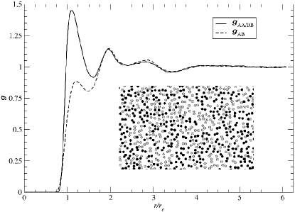
Figure 6: Radial distribution function for the CJ state for $Q=3.0$ eV. $g_{\textrm{AB}}$ measures the chance of finding particles of opposite types a distance $r$ apart divided by the probability if the atoms were randomly distributed. $g_{\textrm{AA/BB}}$ indicates the probability of finding particles of the same type a distance $r$ apart, again, divided by the probability if the distribution were random. The inset shows a section of a snapshot of the simulation. A atoms are black and B are gray.

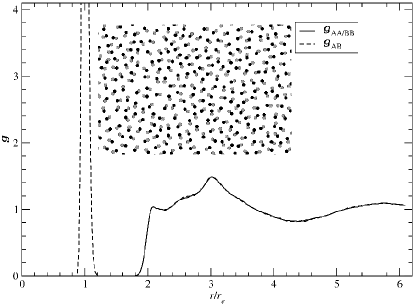
Figure 7: RDF for melted AB. The first peak, the maximum of which is about 14, indicates the presence of dimers. The peak above $r/r_{e}=2$ is due to the inner cutoff spline in the $V_{vdW}$ term of Eq. 1. The peak at $r/r_{e}=3$ is probably caused by the arrangement of dimers.

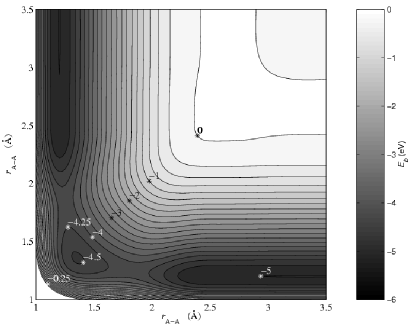
Figure 8: Potential energy in eV vs. separation distances in Å of three inline A (or B) atoms. The “*” marks the contour labeled by the nearby number. Notice the local minimum at (1.3, 1.3). It allows for trimer formation. No positive contours are shows, as would fill in the section near (1,1). The case for inline A-B-A (or B-A-B) looks similar yet shallower.

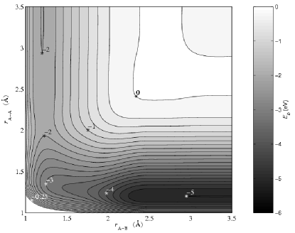
Figure 9: Potential energy vs. separation distances of an A-A-B (or B-B-A) configuration.

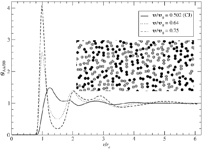
Figure 10: Same-type radial distribution function for an exothermicity $Q=1.5$ eV at states along the Hugoniot at volumes shown. Notice the maximum at radial distance $r/r_{e}\approx 2.75$ for the CJ state. It represents the van der Waals equilibrium distance. The local minimum of the other curves at that point are still greater than unity. Notice the local maxima for the other two curves at $r/r_{e}=3.0$. They suggest tetramer formation or dimer alignment as with the AB melt. The inset is a snapshot of the simulation for $v/v_{0}=0.64$.

IV Exothermicity’s Relationship to EOS

We now turn to understanding the linear relationship between $u_{s}^{2}$ and $Q$. One simple model is suggested by Fickett et al. Fickett and Davis (1979), who derive a linear relationship between $Q$ and $u_{s}^{2}$ by adding $Q$ to the incomplete equation of state of the initial state of a polytropic gas, an ideal gas with a constant specific heat. An expression for the change in specific internal energy becomes $E-E_{0}=(Pv-P_{0}v_{0})/(\gamma-1)-Q$, where $\gamma$ is the adiabatic gamma Davis (1998). One can then eliminate $E-E_{0}$ with the Hugoniot jump condition (Eq. 4), thus solving for $P$. It is assumed that $P_{0}=0$. One can use the condition that Rayleigh line is tangent to the Hugoniot at the CJ state to arrive at $u_{s}^{2}=2(\gamma^{2}-1)Q/m$, where $m$ is the mass of the reactants. If it is assumed that this EOS accurately describes our potential, $\gamma\approx 2$. A typical conventional HE has a $\gamma\approx 3$ Mader (1979). Since the volume at the CJ state is given by the expression $v/v_{0}=\gamma/(\gamma+1)$, this relationship does rationalize the somewhat greater compression observed here ($v/v_{0}<0.67$) compared to that for conventional HE’s ($v/v_{0}\approx 0.75$). (It should be noted that the values of $v/v_{0}$ given in Table 1 are smaller yet and imply a value of $\gamma\approx 1$.) However, as we have demonstrated that the product’s EOS does not behave like an ideal gas, this does not serve as a good basis to explain the observed relationship between $u_{s}^{2}$ and $Q$.

An alternative explanation is suggested by an examination of the Hugoniot curves shown in Fig. 5. There, in the region of $0.55<v/v_{0}<0.7$ (which spans the region containing the CJ states), there appears to be an approximately linear offset of the curves. This suggests that a Mie-Grüneisen EOS with an unspecified reference Hugoniot might be suitable, where it is assumed that the value of $\Gamma/v$ is dependent on $v$. Truncating the Taylor expansion around a reference Hugoniot as in Davis (1998), we get

$$P\approx P_{R}+\Gamma(E-E_{R})/v,$$ (7)

where the Grüneisen gamma

$$\Gamma\equiv v\left(\frac{\partial P}{\partial E}\right)_{v}.$$ (8)

We substitute Eq. 4 into Eq. 7 and, because we take $E$ as relative to the products, set $E_{0}=q$, where $q$ is the specific heat of reaction. Upon rearrangement we get for the $P$-$v$ Hugoniot

$$P_{H}=\frac{1}{v\left(1-\frac{\Gamma}{2}\frac{v_{0}-v}{v}\right)}\left[vP_{R}+\Gamma(q-E_{R})\right].$$ (9)

Rearranging Eqs. 5 and 6, we find

$$u_{s}^{2}=P_{H}\frac{v_{0}}{1-\frac{v}{v_{0}}}.$$ (10)

This yields the general expression

$$u_{s}^{2}=A(v,\Gamma)P_{R}+B(v,\Gamma)(q-E_{R}).$$ (11)

It should be noted that $q$ does not necessarily equal $Q/m$. In the case where the bond order parameter $\overline{B_{ij}}=1.0$ for the initial state, $Q/m$ should be $q$ less the small contribution of the van der Waals interaction. When we run an NVE simulation of 1250 AB molecules at the initial state used in the NEMD simulations, we find a total internal energy of -2548.5 eV. Where Davis measures the zero of energy as cold products Davis (1998), our calculations use a zero of cold dissociated atoms. Our measurement here finds $E_{0}\approx D_{e}^{\textrm{AB}}$ and is consistent with $\overline{B_{ij}}=1.0$ and a 2% van der Waals contribution of a few neighbors, therefore $Q/m\approx q$ to very good order, and the two can be used interchangeably.

The validity of this Mie-Grüneisen approximation can be tested by the linear dependence of $u_{s}^{2}$ on $Q$ for constant volumes. A few of these plots are given in Fig. 11, which shows that good linear relationships are found for the three selected volumes. This shows that the Mie-Grüneisen EOS is a good approximation for our model for low $v$ (high compressions). Since the data were generated during the process of seeking the minimum $u_{s}$ for each $Q$, interpolation was used to find values at common abscissas. The coefficients of the fits generated by the method in Fig. 11 are then plotted in Fig. 12 vs. $v/v_{0}$. Here, $A^{\prime}$ is the y-intercept of those linear fits, and $B$ is the slope. The value $A^{\prime}$ is distinct from $A$ in Eq. 11 because it now includes a contribution from $E_{R}$. However, the value of $B$ is exactly the same as defined in that equation. The fact that all of the lines in Fig. 11 cross at $Q=2.0$ eV leads one to conclude that $A^{\prime}$ and $B$ are linearly dependent. The third curve on Fig. 12 is an attempt to show this for the relation $A^{\prime}=77.5-2.0B$.

The net result of this analysis is that, over the range of $0.55<v/v_{0}<0.7$, $B$ is reasonably constant with a value of 17–19 $(\textrm{km/s})^{2}/$ eV. This result, inserted back into Eq. 11, is then in good agreement with the initial observation shown in Fig. 2, that the slope of the dependence of $u_{s}^{2}$ on $Q$ is $\approx 19\textrm{~{}(km/s)}^{2}/\textrm{eV}$. The ability to approximate the product EOSs as linear Mie-Grüneisen offsets of one another, at least in the region near the CJ states, clarifies the origin of this linear dependence for this system.

Using Eqs. 9, 10, and 11, we can then solve for $\Gamma$ to find

$$\Gamma(v)=\frac{2B\left(1-\frac{v}{v_{0}}\right)\frac{v}{v_{0}}}{2+B\left(1-\frac{v}{v_{0}}\right)^{2}}$$ (12)

and plot the result in Fig. 13. Solving for $B$ we have

$$B(v)=\frac{\Gamma}{\left(1-\frac{v}{v_{0}}\right)\left(1-\frac{\Gamma}{2}\left(1-\frac{v}{v_{0}}\right)\right)}.$$ (13)

Note that $(1-v/v_{0})$ is the compression ($\eta$). From these equations, it can be seen that a constant value of $B$ does not specify a constant value of $\Gamma$, but rather a particular dependence of $\Gamma$ on $v$. Conversely, a constant value of $\Gamma$ would also specify a particular dependence of $B$ on $v$. However, from these two figures it is observed that both $B$ and $\Gamma$ are rather weak functions of $v$ in the CJ region. This aspect of the EOS behavior (which we are unable to directly adjust) is the origin of the linear dependences observed in Fig. 2.

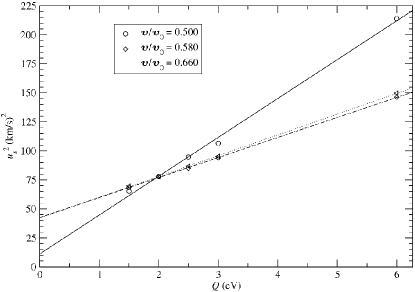
Figure 11: Square of the shock velocity ($u_{s}^{2}$) vs. exothermicity ($Q$) for select constant values of specific volume ($v$). The lines are linear fits. Notice that the fit is better for the higher values of $v$. Notice, also, that the lines cross at $v/v_{0}=2.0$ eV. This indicates a linear dependence between the slopes and the y-intercepts.

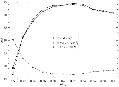
Figure 12: Coefficients of the fits as described in Fig. 11 vs. specific volume for $D_{e}^{\textrm{AB}}=2.0$ eV. $A^{\prime}$ is the y-intercept and, as in Eq. 11, $B$ is the slope. The dashed line is the calculation shown in the legend.

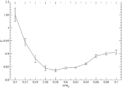
Figure 13: Grüneisen $\Gamma$ vs. specific volume for $D_{e}^{\textrm{AB}}=2.0$ eV.

V Reaction Zone Thickness and Rate Stick Failure Diameter

Having established the steady-state properties of these systems, we now turn to the transient properties related to the reaction zone thickness. There are two means that could be employed to determine the character of the reaction zone for these simulations. The most direct means is to drive the system with a piston whose velocity is matched to that of the CJ conditions. In this case, the one dimensional profile should exhibit a rapid shock rise up to the von Neumann state, followed by a relaxation to the CJ state, which is then a constant zone that extends back to the piston. There will be some transients present because the initiation process incurs a slight delay so that an equilibrium state is not immediately established, but otherwise this is a direct method if the CJ conditions are known. Less direct is to study a system with either an underdriven piston or perhaps initiated with a flyer plate. Such systems will initially propagate at less than the CJ conditions because the release waves can eat into the reaction zone. As the detonation proceeds and the release Taylor wave becomes more spread out (approximating a more steady condition behind the reaction zone), these will eventually “build-up” to a steady detonation. It can be difficult to determine exactly when the system has evolved to a steady-state condition.

A comparison of these two approaches is shown in Fig. 17. For the case of a piston matched to the CJ conditions, a steady solution evolved quite rapidly as determined by both the detonation velocity and the constant properties of the following zone. The reaction zone, defined to be the distance from the shock front to the point where the transient properties are not distinguishable from the thermal fluctuations of the constant zone, extends out to $\approx 300$ Å. A somewhat better characterization is probably the distance at which the particle velocity has decreased to $1/e$ of the initial overshoot. This occurs at $\approx 60$ Å behind the shock front, or a characteristic time constant of 0.7 ps. For the transient simulations, it is apparent that the system is continuing to evolve even after propagating for 100 ps. The reaction zone length (emphasized in the inset) is clearly extending past 100 Å. (The unusual structure after the reaction zone is likely due to the unusual chemical structure of the CJ state, and could be characterized as a phase transition back to the diatomic $\textrm{A}_{2}$ and $\textrm{B}_{2}$ products.) These measurements for the build up time, reaction zone width, and the detonation velocity are larger than those proposed by White et al. White et al. (2000) for the same model. They include in their calculations a time domain in which the detonation is still subtly building. We, in fact, measure a detonation velocity ($9.5580\pm 0.0013$ km/s) close to theirs (9.5 km/s) for the unsupported case if we include the front positions at 10 ps $<t<20$ ps in the linear least-squares fitting that determines $u_{s}$. This highlights the difficulties in using this approach of unsupported detonations.

It should be noted that the transient system exhibits the classic build-up behavior quite nicely. In addition to the extension of the reaction zone out to its equilibrium value, there is also the gradual increase in the initial shock state up to its equilibrium value. As this sets the initial temperature and rate for the reaction chemistry, it emphasizes the significance of these transient phenomena. The shock velocity is also a sensitive indicator of the build-up process. While the deprecation of the velocity below the steady-state value is not great nor readily obvious, it can be discerned by careful observation. Previously reported discrepancies between expected and observed CJ performance may well have been due to systems not having fully attained steady-state conditions.

In Davis (1981) Davis shows that surface effects adversely affect detonation’s ability to propagate because rarefaction waves from the side release erode the reaction zone and its support structure. For cylindrical charges, this is characterized as a failure diameter below which detonation cannot propagate. White et al. report that, when the periodic boundaries are removed from the sample so that the particles are free to escape the system, there is a critical width ($W_{c}$) that the sample must exceed in $\hat{x}$, the direction perpendicular to the propagation of the shock front, in order that the detonation be sustained. If the sample is too thin, rarefaction waves quench the detonation White et al. (2000).

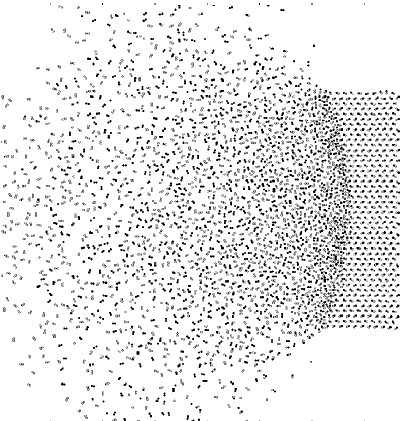
Figure 14: Rate stick at super-critical width.

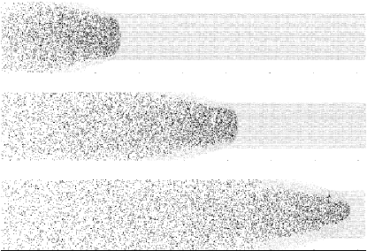
Figure 15: Three sequential snapshots of a rate stick at sub-critical width. Here the particles are colored by bond type. Gray is unreacted, and black is reacted. Rarefaction waves from the rate stick’s edge erode at the reaction zone thus quenching the detonation.

$W_{c}$’s dependence on $Q$ Haskins et al. (1998) and $D_{e}^{\textrm{AB}}$ can be seen in Fig. 16. Unlike in Haskins et al. (1998), a curve of the form $y=a/(x-Q_{c})$, not exponential, is fit to the data for $Q$. Simpler equations fit better, but this form is inspired by Hubbard and Johnson’s Hubbard and Johnson (1959) dependence of delay time ($t_{d}$) (described below) on $Q$ and to be asymptotic at the point where detonation is known to fail for an infinitely thick sample ($Q_{c}$). For $D_{e}^{\textrm{AB}}$ a curve of the form $y=a(e^{bx}-1)/(x-D_{ec}^{\textrm{AB}})$ is fit to the data for similar reasons. If $Q$ is raised, the reaction should be more difficult to quench because there is more energy available to break neighboring AB bonds. The reaction is expected to be faster and the reaction zone shorter because of the higher temperature resulting from the greater energy release. As $Q$ lowers toward $Q_{c}$, no matter how wide the sample is, detonation will not be sustained. On the other hand, if $D_{e}^{\textrm{AB}}$ is lowered, it is harder for rarefaction waves to quench the detonation front because, with a lower dissociation energy, a chemical reaction occurs more readily. $W_{c}$ is, thus, lowered because detonation is more easily sustained. As it rises, $D_{e}^{\textrm{AB}}$ reaches a critical value ($D_{ec}^{\textrm{AB}}$) (probably dependent on $Q$, flyer thickness and velocity, etc.) above which detonation cannot be sustained, no matter how wide the sample.

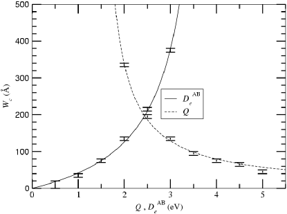
Figure 16: Critical width ($W_{c}$) vs. AB dissociation energy ($D_{e}^{\textrm{AB}}$) and exothermicity ($Q$). The upper dash of the error bar indicates the thinnest sample to sustain detonation. The lower error bar indicates the thickest sample to fail within 360 lattice spaces. The resolution is 10 Å. The lines are guides to the eye with empirical functional forms discussed in the text.

In a sample with culled boundaries, if $D_{e}^{\textrm{AB}}$ is lowered, it is harder for rarefaction waves to quench the detonation front because, with a lower dissociation energy, a chemical reaction occurs more readily. $W_{c}$ is, thus, lowered because detonation is more easily sustained. As it rises, $D_{e}^{\textrm{AB}}$ reaches a critical value ($D_{ec}^{\textrm{AB}}$) (probably dependent on $Q$, flyer thickness and velocity, etc.) above which detonation cannot be sustained, no matter how wide the sample.

Using the idea of delay time ($t_{d}$), during which a reactant must remain above a certain temperature in order for a reaction to occur, Hubbard et al. give an example of how a detonation’s ability to be initiated or sustained may depend on $Q$ and $D_{e}^{\textrm{AB}}$. We use this in lieu of finding reaction rate data. The longer this time, the less likely the reaction. In their example, $t_{d}$ has an inverse dependence on $Q$ and an inverse and exponential dependence on activation energy, $E_{a}$ (Eq. 14) Hubbard and Johnson (1959).

$$t_{d}=\frac{RE^{2}_{0}}{c_{v}\nu E_{a}Q}\exp\left(\frac{c_{v}E_{a}}{RE_{0}}\right),$$ (14)

where $\nu$ is the collision rate, $R$ is the molar gas constant, $c_{v}$ is the specific heat at constant volume, and $E_{0}$ is the internal energy behind the shock.

In Rosing and Chariton theory, when $\Theta=t_{r}$, $d=W_{c}$, where $\Theta$ is scattering time, $t_{r}$ is the reaction time, and $d$ is the diameter of the sample. The rate stick must be thick enough that rarefaction waves, traveling at $c$ from the surface, cannot sufficiently penetrate the HE in order to scatter the reaction zone and quench the reaction in a time equal to the reaction time. $a=t_{r}(u_{s}-\bar{u})$, where $a$ is the width of the chemical reaction zone, $\bar{u}$ is the average particle velocity in $\hat{z}$ within the zone, and $u_{s}$ is the velocity of the detonation front. $\Theta=d/2c$, where $c$ is the speed of sound. Replacing $t_{r}$ with $\Theta$, one finds

$$W_{c}=d=2ca/(u_{s}-\bar{u}),$$ (15)

where $u_{s}$ is a function of $d$ Dremin (1999); White et al. (2001); Davis (1981). If $t_{d}\propto t_{r}$ and $E_{a}\propto D_{e}^{\textrm{AB}}$, we find that $W_{c}\propto t_{d}$, supporting our selection of curve fits.

(a)

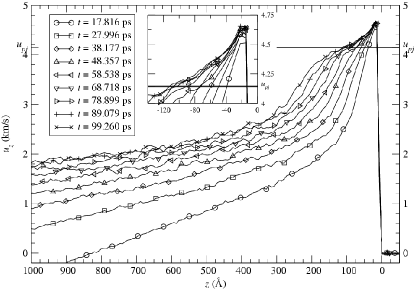
(b)

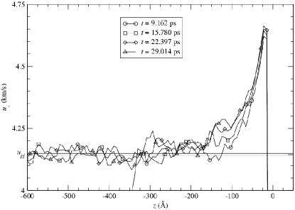
Figure 17: (a) 129 profiles of the particle velocity on the z direction ($u_{z}$) separated in time by 50.9 fs are overlapped onto their center profile (whose time is indicated in the legend) such that their fronts line up. They are averaged and those averages are similarly overlapped. The simulation represented has the default parameterization for the REBO potential Brenner et al. (1993). It is a flyer driven unsupported simulation as described in Sec. II. Found for this specific parameterization in Sec. IV, $u_{pj}$ is indicated by a constant line segment. The inset is a magnification of the region containing the von Neumann spike and the CJ state.
(b) Similar profiles for a critically supported detonation. This simulation is shorter and thinner than in (a), but it suggests that in (a) still has some building to do for the profiles do not seem to settle down to $u_{pj}$ until about 300 Å behind the front.

To check the validity of Eq. 15, we use for $a$ the characteristic decay length of the reaction zone (60 Å) determined above. If the ratio $2c/(u_{s}-\bar{u})\sim 2$, this would be excellent agreement. As the value of $u_{s}-\bar{u}$ should be approximately equal to the local sound speed, this estimation is then quite good. Given the approximations involved in making this assessment, this is certainly a fortuitous agreement, but can be taken as support for this analysis. Overall, a more thorough understanding of these phenomena is evolving through these studies.

VI Conclusion

We have analyzed the relationships between the energetic chemical properties of a simple, but well studied, model high explosive and the physical properties of its detonation front through explicit Molecular Dynamics (MD). This provides an excellent means to compare to continuum analyses and avoids the complication of a multiphase equation of state (EOS) and other approximations required in those approaches. Most previous MD studies of high explosives have focused on the physical properties of the HE as independent parameters (e.g. voids and gaps) to validate this general approach. Our analysis has been conducted in order to establish a more quantitative comparison to the relevant theories by, e.g., seeking the CJ state via NVE simulations and showing that it accurately predicts detonation properties such as the detonation velocity ($u_{s}$). Despite spurious model anomalies, e.g., a CJ state consisting of polyatomic species and unusual properties of the product Hugoniot curves, we have observed general consistency between the MD approach and the thermodynamic equations. Given that the fundamental CJ and ZND models pose minimal constraints on the behavior of chemical system, this result is not extremely surprising. However, we have demonstrated that it is possible to gain a quantitative understanding of these relationships even for these somewhat unusual systems. For the analysis of the behavior of $u_{s}$ and the critical width as functions of energetic parameters, we have explained our results in the context of available theories. In the case of $u_{s}^{2}$ as a function of the dissociation energy of AB, we have not directly determined the reason for its linear and increasing relationship, but assume that it also determined by the induced EOS changes. In characterizing the reaction zone width, we demonstrated that transient simulations must be scrutinized rather carefully in determining the final state. We are currently investigating the sources of the model anomalies that we have identified, and potential model revisions that will correct these are expected to result in a system that behaves more similarly to conventional high explosives.