On-site approximation for spin-orbit coupling in LCAO density functional methods

Abstract

We propose a computational method that simplifies drastically the inclusion of spin-orbit interaction in density functional theory when implemented over localised atomic orbital basis sets. Our method is based on a well-known procedure for obtaining pseudopotentials from atomic relativistic ab initio calculations and on an on-site approximation for the spin-orbit matrix elements. We have implemented the technique in the SIESTA[34] code, and show that it provides accurate results for the overall band structure and splittings of group IV and III-IV semiconductors as well as for 5$d$ metals.

J. Phys.: Condens. Matter18 7999-8013, 2006

1 Introduction

Computational methods in condensed matter physics are a powerful tool for predicting and explaining the most diverse properties of materials, nanostructures and small biological systems. Among an enormous plethora of methodologies, density functional theory (DFT) [18, 25] has become a standard for simulations at the atomic and nanometric scale. Several numerical implementations of DFT are available and the details of the algorithm usually depends on the specific applications the method is designed for. These implementations can be categorized according to two different schemes.

The first scheme divides DFT codes depending on the basis functions used, namely plane-waves or linear combination of atomic orbitals (LCAO). Plane waves are typically easier to implement and the convergence is determined by a single variational parameter, the energy cutoff. In contrast LCAO implementations are based on a tight binding description of the chemical bond. They are more cumbersome to implement and the variational principle is controlled by a set of parameters defining the basis functions. However these second methods are ideal for linear scaling since sparse Hamiltonian can be constructed by using strictly confined orbitals [17].

The second classification takes into account whether the codes simulate both core and valence electrons or only the valence ones. In the first case the method is regarded as all electron since all the electronic degrees of freedom are treated on the same footing. This for instance allows one to perform fully relativistic calculations without any conceptual complication. All electron methods are remarkably accurate but have the drawback that the calculations are usually rather intensive and only relatively small systems can be tackled. In the second case the contribution of the core electrons is casted into pseudopotentials [27], which also can be constructed from DFT. This reduces drastically the number of electrons considered in the self-consistent simulation and much larger systems can be investigated.

Spin-orbit interaction is a relativistic effect whose magnitude increases with the atomic number. Consequently it provides negligible contributions to the electronic structure of individual atoms and bulk materials made of light elements. However it has a significant impact over the physics of heavier elements, for instance 3$d$ ferromagnetic materials. Spin-orbit can produce magnetic anisotropies of the order of 10 to 100 $\mu$eV for bcc and fcc Fe, Ni and Co [7], therefore is the underlying mechanism for establishing the magnetic easy and hard axes and for controlling the shape of domain walls [6]. It is also the primary interaction responsible for most of the zero field splitting and other properties of magnetic molecules [16].

In semiconductors spin-orbit interaction spin-splits the edges of the valence and the conduction band [40] and allows electrical manipulation of the spin-direction [10]. This last effect is of paramount importance for the growing field of spintronics [39], which has certainly added more impetus to the inclusion of the spin-orbit interaction in the description of the electronic structure. Spin-orbit coupling determines the spin-relaxation time of electrons in ordinary semiconductors and in semiconductor heterostructures, [21] and also plays an important role in the physics of diluted magnetic semiconductors. [35] Finally is worth mentioning that electron spin manipulation using spin-orbit interaction was recently demonstrated in the so-called spin-Hall effect [20], a solid state version of the Stern-Gerlach measurement.

It is therefore clear that spin-orbit interaction is becoming increasingly important for a number of applications, which also require the description of rather large systems. This calls for an efficient implementation of spin-orbit within pseudopotential LCAO based algorithms. Interestingly most of the mainstream LCAO codes such as SIESTA [34], Onetep [33], Fireball [32] and Conquest [9] do not contain implementations of spin-orbit interaction in their present form. In contrast quantum chemistry packages such as Gaussian[12] or Turbomole [28] are not equipped for solid-state simulations.

Therefore we have developed a general method for including spin-orbit interaction in conventional pseudopotential based LCAO DFT methods. This is not computationally demanding and hence it is fully adequate for large scale simulations. The method, although not suitable for highly accurate total energy calculations for which all electron plane-wave schemes cannot be matched, provides an excellent description of the effects of spin-orbit coupling on the electronic structure. Here we describe our implementation within the SIESTA program, [34] although the scheme is very general and it could be readily implemented in any LCAO pseudopotential codes with non-collinear electron spin functionalities. [29, 15]

The paper is organized as follows: we first present the details of the method, our numerical implementation and numerical tests of one- and two-center integrals (section III). We then demonstrate the capability of the proposed scheme with predictions for group IV and III-V semiconductors and for 5$d$ metals (sections IV and V, respectively).

2 The On-site approximation

2.1 Relativistic effects in pseudopotential methods

Kleinman and Bylander have shown that the procedures for generation of non-relativistic pseudopotentials can be easily extended to account for relativistic effects. [23, 5] This relies on solving self-consistently the all-electrons Dirac equation for a single atom and in the extraction of a pseudopotentials $V_{j}$, where now $j$ is the total angular momentum $j=l\pm\frac{1}{2}$. The pseudopotential Hamiltonian can therefore be written as

$$\hat{V}=\sum\limits_{j,m_{j}}|j,m_{j}\rangle\,V_{j}\,\langle j,m_{j}|,$$ (1)

and includes all relativistic corrections to order $\alpha^{2}$, where $\alpha$ is the fine structure constant and $|j,m_{j}\rangle$ are total angular momentum states. This expression can be recast in a form suitable for non-relativistic pseudopotential theory by expressing $|j,m_{j}\rangle$ in terms of a tensor product of the regular angular momentum states $|l,m\rangle$ and the eigenstates of the $z$ component of the Pauli spin matrices[31]

$$|j=l+\frac{1}{2},m_{j}\rangle = \left(\begin{array}[]{c}\sqrt{\frac{l+m_{j}+\frac{1}{2}}{2l+1}}\,\,|l,m_{j}-\frac{1}{2}\rangle\\ \sqrt{\frac{l-m_{j}+\frac{1}{2}}{2l+1}}\,\,|l,m_{j}+\frac{1}{2}\rangle\end{array}\right),$$ (4)

$$|j=l-\frac{1}{2},m_{j}\rangle = \left(\begin{array}[]{c}\sqrt{\frac{l-m_{j}+\frac{1}{2}}{2l+1}}\,\,|l,m_{j}-\frac{1}{2}\rangle\\ -\sqrt{\frac{l+m_{j}+\frac{1}{2}}{2l+1}}\,\,|l,m_{j}+\frac{1}{2}\rangle\end{array}\right).$$ (7)

Equation (1) can then be rewritten[1] as

$$\hat{\mathbf{V}} = \hat{\mathbf{V}}^{sc}+\hat{\mathbf{V}}^{SO}=$$ (8)

$$= \sum\limits_{l,m}\,[\,\bar{V}_{l}\,\leavevmode\hbox{\small 1\kern-3.8pt\normalsize 1}_{\sigma}+\bar{V}_{l}^{SO}\vec{L}\cdot\vec{\mathbf{S}}\,]\,\,|l,m\rangle\langle l,m|,$$

where we use bold letters to indicate 2x2 matrices, with $\leavevmode\hbox{\small 1\kern-3.8pt\normalsize 1}_{\sigma}$ representing the unit operator in spin space,

$$\vec{L}\cdot\vec{\mathbf{S}}=\frac{1}{2}\left(\begin{array}[]{cc}\hat{L}_{z}&\hat{L}_{-}\\ \hat{L}_{+}&-\hat{L}_{z}\end{array}\right),$$ (9)

and,

$$\bar{V}_{l}^{\phantom{SO}} = \frac{1}{2l+1}[(l+1)V_{l+\frac{1}{2}}+lV_{l-\frac{1}{2}}],$$

$$\bar{V}_{l}^{SO} = \frac{2}{2l+1}[V_{l+\frac{1}{2}}-V_{l-\frac{1}{2}}].$$ (10)

It should be stressed that the scalar part $\hat{\mathbf{V}}^{sc}$ of the pseudopotential contains now not only the conventional non-relativistic pseudopotential, but also the scalar relativistic corrections.

The vectors $|l,m\rangle$, representing complex spherical harmonics, form a complete basis for the Hilbert space of the angular momentum operator $\vec{L}$. It is a useful practice in solid state physics and quantum chemistry to replace them with real spherical harmonics $|l,M\rangle$, since the corresponding Hamiltonian is a real matrix. The change of basis is achieved by the following unitary transformation

$$|l,M\rangle = \frac{1}{\sqrt{2}}\,\left(\,|l,m\rangle+(-1)^{m}\,|l,\overline{m}\,\rangle\right),$$

$$|l,\overline{M}\,\rangle = \frac{1}{\sqrt{2}\,i}\,\left(\,|l,m\rangle-(-1)^{m}\,|l,\overline{m}\,\rangle\right),$$ (11)

which is valid for $M>0$ ($\,\overline{M}=-M$, $\overline{m}=-m$). The case $M=0$ is simply given by $|l,M=0\rangle=|l,m=0\rangle$.

The pseudopotential operator $\hat{\mathbf{V}}$ of equation (8), is now written as

$$\hat{\mathbf{V}} = \hat{\mathbf{V}}^{sc}+\hat{\mathbf{V}}^{SO}=$$ (12)

$$= \sum\limits_{l,M}[\,\bar{V}_{l}\,\leavevmode\hbox{\small 1\kern-3.8pt\normalsize 1}_{\sigma}+\bar{V}_{l}^{SO}\vec{L}\cdot\vec{\mathbf{S}}\,]|l,M\rangle\langle l,M|\;.$$

Finally the Kohn-Sham Hamiltonian [25] is expressed as a sum of kinetic energy $\hat{\mathbf{T}}$, scalar relativistic $\hat{\mathbf{V}}^{sc}$, spin-orbit $\hat{\mathbf{V}}^{SO}$, Hartree $\hat{\mathbf{V}}^{H}$ and exchange and correlation $\hat{\mathbf{V}}^{xc}$ potentials

$$\hat{\mathbf{H}}=\hat{\mathbf{T}}+\hat{\mathbf{V}}^{sc}+\hat{\mathbf{V}}^{SO}+\hat{\mathbf{V}}^{H}+\hat{\mathbf{V}}^{xc}\;.$$ (13)

This Hamiltonian is therefore a $2\times 2$ matrix in spin space

$$\hat{\mathbf{H}}=\left[\begin{array}[]{cc}\hat{H}^{\uparrow\uparrow}&\hat{H}^{\uparrow\downarrow}\\ \hat{H}^{\downarrow\uparrow}&\hat{H}^{\downarrow\downarrow}\end{array}\right],$$ (14)

whose non-diagonal blocks arise from the exchange and correlation potential whenever the system under consideration displays a non-collinear spin, and also from the spin-orbit potential.[29, 15]

2.2 Spin-orbit in LCAO schemes: the on-site approximation

LCAO methods expand the eigenstates $|\psi_{n}\rangle$ of the non-collinear Kohn-Sham Hamiltonian over a set of localised orbitals $|\phi_{i}\rangle$,

$$|\mathbf{\psi}_{n}\rangle=\sum_{i}\left(\begin{array}[]{c}c_{n,i}^{\uparrow}\\ c_{n,i}^{\downarrow}\end{array}\right)\,\,|\phi_{i}\rangle$$ (15)

where $i$ is a collective index for all the symbols required to describe uniquely a given orbital

$$|\phi_{i}\rangle=|\phi_{n_{i},l_{i},M_{i}}\rangle=|R_{n_{i},l_{i}}\rangle\otimes\,|l_{i},M_{i}\rangle\>.$$ (16)

Here both the radial and angular part of the wave function $\phi_{i}(\vec{r}-\vec{d}_{i})=\langle\vec{r}\ |\phi_{i}\rangle$ is centered at the position $\vec{d}_{i}$. Note that $n_{i}$ does not necessarily describe the principle quantum number only, but generally labels a set of radial functions associated to the angular momentum $l_{i}$ according to the multiple zetas scheme.[30]

The Kohn-Sham equation, $\hat{H}\,|\psi_{n}\rangle=E_{n}\,|\psi_{n}\rangle$, is then projected onto such orbital basis set as

$$\left[\begin{array}[]{c c}H^{\uparrow\uparrow}_{ij}-E_{n}S_{ij}&H^{\uparrow\downarrow}_{ij}\\ H^{\downarrow\uparrow}_{ij}&H^{\downarrow\downarrow}_{ij}-E_{n}S_{ij}\end{array}\right]\,\left[\begin{array}[]{c}c_{n,j}^{\uparrow}\\ c_{n,j}^{\downarrow}\end{array}\right]=0,$$ (17)

where $H^{\sigma\sigma^{\prime}}_{ij}=\langle\phi_{i}|\hat{H}^{\sigma\sigma^{\prime}}|\phi_{j}\rangle$ and $S_{ij}=\langle\phi_{i}|\phi_{j}\rangle$ are the matrix elements of the Hamiltonian and overlap matrix respectively.

The spin-orbit term can then be calculated as

$$\mathbf{V}^{SO}_{ij} = \langle\phi_{i}|\hat{\mathbf{V}}^{SO}|\phi_{j}\rangle=$$ (18)

$$= \!\!\!\!\sum\limits_{k,l_{k},M_{k}}\!\!\!\langle\phi_{i}|\bar{V}_{l_{k}}^{SO}\vec{L}\cdot\vec{\mathbf{}S}\,|l_{k},M_{k}\rangle\,\langle l_{k},M_{k}|\phi_{j}\rangle,$$

where index $k$ indicates the atom on which the potential is centered, $\bar{V}_{l_{k}}^{SO}=\bar{V}_{l}^{SO}(\vec{r}-\vec{d}_{k})$ and $|l_{k},M_{k}\rangle$ is the spherical harmonic centered at the same atomic position ${\vec{d}}_{k}$. Equation (18) involves a considerable number of three-center integrals. Inclusion of the spin-orbit interaction is therfore, in the LCAO approach, if straightforward, computationally intensive. One possibility of reducing the computational effort is to construct fully non-local pseudopotentials. [24] We note however that the radial part of the spin-orbit pseudopotentials, $\bar{V}^{SO}_{l}$, is very short-ranged, resulting in matrix elements that decay quickly with the distance among the three centers. Thus we consider only matrix elements where the three components, both orbitals and the pseudopotential, reside on the same atom, and discard all the rest. This approximation simplifies the matrix elements of equation (18) to one center integrals and drastically reduces the computational effort needed to account for spin-orbit effects. Then our approximated matrix elements are

$${\mathbf{V}}^{SO}_{ij} = \frac{1}{2}\sum\limits_{k,l_{k}>0,M_{k}}\langle R_{n_{i},l_{i}}|\bar{V}_{l_{k}}^{SO}|R_{n_{j},l_{j}}\rangle\,\langle l_{i},M_{i}|\left(\begin{array}[]{cc}\hat{L}_{z}&\hat{L}_{-}\\ \hat{L}_{+}&-\hat{L}_{z}\end{array}\right)\,|l_{k},M_{k}\rangle\,\langle l_{k},M_{k}|l_{j},M_{j}\rangle$$ (21)

$$\approx \frac{1}{2}\,\langle R_{n_{i},l_{i}}|\bar{V}_{l_{i}}^{SO}|R_{n_{j},l_{i}}\rangle\,\langle l_{i},M_{i}|\left(\begin{array}[]{cc}\hat{L}_{z}&\hat{L}_{-}\\ \hat{L}_{+}&-\hat{L}_{z}\end{array}\right)\,|l_{i},M_{j}\rangle\,\delta_{l_{i},l_{j}},$$ (24)

since the $\hat{L}_{\alpha}$ operators leave each $l_{i}$ subspace invariant. The angular part of these on-site matrix elements can be calculated analytically

$$\langle l,M_{i}|\hat{L}_{z}|l,M_{j}\rangle = -iM_{i}\delta(M_{i}+M_{j}=0)$$ (25)

$$\langle l,0|\hat{L}_{\mp}|l,M_{j}\rangle = \pm\sqrt{\frac{l(l+1)}{2}}\delta(M_{j}=1)-i\sqrt{\frac{l(l+1)}{2}}\delta(M_{j}=\bar{1})$$

$$\langle l,1|\hat{L}_{\mp}|l,M_{j}\rangle = -i\frac{\sqrt{l(l+1)-2}}{2}\delta(M_{j}=\bar{2})\mp\sqrt{\frac{l(l+1)}{2}}\delta(M_{j}=0)\pm\frac{\sqrt{l(l+1)-2}}{2}\delta(M_{j}=2)$$

$$\langle l,\bar{1}|\hat{L}_{\mp}|l,M_{j}\rangle = \pm\frac{\sqrt{l(l+1)-2}}{2}\delta(M_{j}=\bar{2})+i\sqrt{\frac{l(l+1)}{2}}\delta(M_{j}=0)+i\frac{\sqrt{l(l+1)-2}}{2}\delta(M_{j}=2)$$

$$\langle l,2|\hat{L}_{\mp}|l,M_{j}\rangle = -i\frac{\sqrt{l(l+1)-6}}{2}\delta(M_{j}=\bar{3})-i\frac{\sqrt{l(l+1)-2}}{2}\delta(M_{j}=\bar{1})$$

$$\mp\frac{\sqrt{l(l+1)-2}}{2}\delta(M_{j}=1)\pm\frac{\sqrt{l(l+1)-6}}{2}\delta(M_{j}=3)$$

$$\langle l,\bar{2}|\hat{L}_{\mp}|l,M_{j}\rangle = \pm\frac{\sqrt{l(l+1)-6}}{2}\delta(M_{j}=\bar{3})\mp\frac{\sqrt{l(l+1)-2}}{2}\delta(M_{j}=\bar{1})$$

$$+i\frac{\sqrt{l(l+1)-2}}{2}\delta(M_{j}=1)+i\frac{\sqrt{l(l+1)-6}}{2}\delta(M_{j}=3)$$

$$\langle l,3|\hat{L}_{\mp}|l,M_{j}\rangle = -i\frac{\sqrt{l(l+1)-12}}{2}\delta(M_{j}=\bar{4})-i\frac{\sqrt{l(l+1)-6}}{2}\delta(M_{j}=\bar{2})$$

$$\mp\frac{\sqrt{l(l+1)-6}}{2}\delta(M_{j}=2)\pm\frac{\sqrt{l(l+1)-12}}{2}\delta(M_{j}=4)$$

$$\langle l,\bar{3}|\hat{L}_{\mp}|l,M_{j}\rangle = \pm\frac{\sqrt{l(l+1)-12}}{2}\delta(M_{j}=\bar{4})\mp\frac{\sqrt{l(l+1)-6}}{2}\delta(M_{j}=\bar{2})$$

$$+i\frac{\sqrt{l(l+1)-6}}{2}\delta(M_{j}=2)+i\frac{\sqrt{l(l+1)-12}}{2}\delta(M_{j}=4)$$

Some useful symmetries of the matrix elements of the Hamiltonian and of its spin-orbit part should also be highlighted. Since the Hamiltonian is hermitian the matrix elements satisfy the relation

$$H_{ij}^{\sigma\sigma^{\prime}}=(H_{ji}^{\sigma^{\prime}\sigma})^{*}.$$ (26)

Moreover it is also easy to show that all the terms in the Hamiltonian satisfy a spin box hermiticity, i.e.

$$H_{ij}^{\sigma\sigma^{\prime}}=(H_{ij}^{\sigma^{\prime}\sigma})^{*},$$ (27)

except for the spin-orbit contribution which is spin box anti-hermitian

$$H_{ij}^{\sigma\sigma^{\prime}}=-(H_{ij}^{\sigma^{\prime}\sigma})^{*}.$$ (28)

This property has important consequences for the calculation of the total energy.

2.3 Density matrix and total energy

The charge density can also be written in terms of the LCAO basis as

$$\mathbf{n}(\vec{r}) = \sum_{n}\,\,f_{n}\,\mathbf{\psi}_{n}(\vec{r})\,\,\mathbf{\psi}_{n}(\vec{r})^{\dagger}=$$ (29)

$$= \sum_{i,j}\phi_{i}(\vec{r}-\vec{d}_{i})\,\phi_{j}^{*}(\vec{r}-\vec{d}_{j})\,\,\mathbf{\rho}_{ij}$$

where $f_{n}$ represents the occupation of the Kohn-Sham eigenstate $\psi_{n}(\vec{r}\,)$ and $\mathbf{\rho}_{ij}$ is a $2\times 2$ matrix containing the products of wave-function coefficients, whose components are

$$\rho_{ij}^{\sigma\sigma^{\prime}}=\sum\limits_{n}\,f_{n}\,\,c_{n,i}^{\sigma}\,c_{n,j}^{\sigma^{\prime}*}.$$ (30)

The electronic contribution to the total energy may be expressed as a sum of a band-structure (BS) contribution plus double-counting corrections. The BS contribution can be written in the LCAO basis as

$$E_{e}^{BS}=\sum\limits_{n}f_{n}\,\,\langle\mathbf{\psi}_{n}|\hat{\mathbf{H}}|\mathbf{\psi}_{n}\rangle=\sum\limits_{i,j,\sigma,\sigma^{\prime}}H_{ij}^{\sigma\sigma^{\prime}}\rho_{ji}^{\sigma^{\prime}\sigma},$$ (31)

which may also be expressed as

$$\sum\limits_{ij}\left\{H_{ij}^{\uparrow\uparrow}\,\rho_{ji}^{\uparrow\uparrow}+H_{ij}^{\downarrow\downarrow}\,\rho_{ji}^{\downarrow\downarrow}+\right.$$

$$\left.+2\,\mathrm{Re}\left[(V_{ij}^{xc\uparrow\downarrow}-V_{ij}^{SO\uparrow\downarrow})\,(\rho_{ji}^{\uparrow\downarrow})^{*}\right]\right\}\>,$$ (32)

where we have isolated the non-diagonal contributions in spin space. These arise only from the spin-orbit interaction and from the exchange and correlation potential whenever spin non-collinearity is present. The spin-orbit contribution to the total energy therefore is

$$E^{SO}=\mathrm{Tr}\sum_{i,j}\mathbf{V}^{SO}_{ij}\,\mathbf{\rho}_{ji},$$ (33)

since there are no double-counting terms.

2.4 Forces and stresses

One important consequence of the on-site approximation is that spin-orbit does not give rise to an explicit contribution to forces and stresses, even though an implicit contribution due to the modification of the self-consistent wave-function is always present. According to Hellmann-Feynman theorem, [13] the spin-orbit contribution to the forces excerpted upon an atom centered at position $\vec{d}_{k}$ is obtained by simply differentiating the energy with respect to the atomic coordinates of the atom,

$$-\vec{F}_{k}^{SO} \!\!=\!\! \vec{\nabla}_{k}E^{SO}=$$ (34)

$$\!\!=\!\! \mathrm{Tr}\sum_{i,j}\!\!\left\{\!\left[\vec{\nabla}_{k}\hat{\mathrm{V}}^{SO}_{ij}\right]\!\mathbf{\rho}_{ji}\!+\!\mathbf{V}^{SO}_{ij}\!\!\,\left[\vec{\nabla}_{k}\hat{\mathrm{\rho}}_{ji}\right]\!\right\},$$

where both the $i$ and $j$ orbitals are centered at the same atomic position $\vec{d}_{k}$ and $\vec{\nabla}_{k}=\vec{\nabla}_{\vec{d}_{k}}$. However both contributions to the spin-orbit forces in equation (34) vanish. The first one is identically zero since the one-center integrals do not depend on the atomic position,

$$\nabla_{k}\langle R_{n_{i},l_{i}}|\bar{V}_{l_{k}}^{SO}|R_{n_{j},l_{j}}\rangle\equiv 0\>.$$ (35)

The second term may be rewritten as

$$-\sum_{ij}\left(\mathcal{E}^{SO,\uparrow\uparrow}_{ij}+\mathcal{E}^{SO,\downarrow\downarrow}_{ij}\right)\vec{\nabla}_{k}{S}_{ji},$$ (36)

where $\mathcal{E}^{SO,\sigma\sigma^{\prime}}_{ij}$ are the components of the spin-orbit contribution to the energy-density matrix

$$\mathcal{E}_{ij}^{SO}=\frac{1}{2}\,\sum\limits_{l,m}\,(S_{il}^{-1}\,\mathbf{V}^{SO}_{lm}\,\mathbf{\rho}_{mj}+\mathbf{\rho}_{il}\,\mathbf{V}^{SO}_{lm}\,S_{mj}^{-1}).$$ (37)

However, since $\mathcal{E}^{SO}$ is antisymmetric with respect to the orbital indices, in contrast to the overlap matrix that is symmetric, the second term vanishes as well.

In a similar way one can demonstrate that the spin-orbit interaction in the on-site approximation does not introduce any additional contribution to the stress.

3 Numerical tests on one- and two-center integrals

The validity of the on-site approximation relies on the fact that two and three center integrals are much smaller than the one-center ones, which are kept in the simulation. Among those two and three center matrix elements the two-center integrals

$$\mathbf{V}^{2c}_{ij}(\vec{R})=\langle\phi_{i}(\vec{R})\,|\bar{V}_{l_{j}}^{SO}(0)\,\vec{L}(0)\cdot\vec{\mathbf{}S}(0)\,|\phi_{j}(0)\rangle,$$ (38)

are expected to have the largest absolute value. An excellent test consists of calculating these matrix elements for a given material along the direction that joins one atom with its nearest neighbours, as a function of the distance $R$ between the two centers. Then, $R=0$ provides the on-site matrix elements, while if $R$ equals the nearest neighbours distance, the calculation describes the desired two-center integrals. We have performed such test for a representative semiconductor, Si, and a representative 5$d$ metal, Pt.

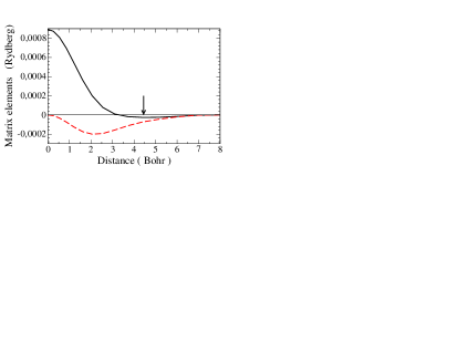
Figure 1: Two-center integrals $\mathbf{V}_{y-x}^{z}(R)$ and $\mathbf{V}_{z-x}^{z}(R)$ (solid and dashed lines, respectively) for silicon along the (111) direction, as a function of the distance R between the two centers. The arrow indicates the distance of the nearest-neighbour atoms.

For silicon, the valence electrons include s- and p-orbitals only and therefore we consider the following matrix elements

$$\mathbf{V}_{y-x}^{z}(R) = \langle\phi_{p_{y}}(R)\,|\bar{V}_{p}^{SO}(0)\,L_{z}(0)\,|\phi_{p_{x}}(0)\rangle\>,$$

$$\mathbf{V}_{z-x}^{z}(R) = \langle\phi_{p_{z}}(R)\,|\bar{V}_{p}^{SO}(0)\,L_{z}(0)\,|\phi_{p_{x}}(0)\rangle\>.$$ (39)

For $R$ =0, the first of these matrix elements reduces to the on-site integral $\mathbf{V}_{y-x}^{z}(0)$, while the second is zero by symmetry. Fig. 1 shows the matrix elements as a function of R along the direction (111). The matrix elements, evaluated at the nearest neighbour distance are considerably smaller than the on-site integral, with the $\mathbf{V}(R)/\mathbf{V}(0)$ ratio being $\sim$0.03 and $\sim$0.08 respectively for $y-x$ and $z-x$.

In the case of Pt we have considered not only the 5$d$ but also the 6$p$ orbitals. Platinum crystalizes with an fcc structure and a nearest neighbours distance of 5.4 a.u. We compute the same $p$-matrix elements as for silicon, as well as the two following $d$ integrals

$$\mathbf{V}_{x^{2}y^{2}-xy}^{z}(R) = \langle\phi_{x^{2}-y^{2}}(R)\,|\bar{V}_{d}^{SO}(0)\,L_{z}(0)\,|\phi_{xy}(0)\rangle\>,$$

$$\mathbf{V}_{z^{2}-xz}^{z}(R) = \langle\phi_{3z^{2}-r^{2}}(R)\,|\bar{V}_{d}^{SO}(0)\,L_{z}(0)\,|\phi_{xz}(0)\rangle\>.$$ (40)

Fig. 2 shows these matrix elements as a function of $R$. For the $d$-type matrix elements (figure 2a) the decay with the distance between the centers is rather dramatic and the two-center matrix elements are about $10^{-4}$ times smaller than the on-site integrals. The case of the $p$-integrals (figure 2b) is similar to that of Si with a $\mathbf{V}(R)/\mathbf{V}(0)$ ratio of $\sim 0.08$. For the specific case of Pt however these $p$-integrals are expected to contribute little to any physical quantities since they correspond to unoccupied states.

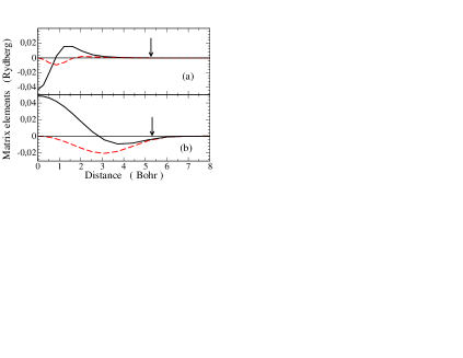
Figure 2: (a) Two-center integral $\mathbf{V}_{x^{2}-y^{2}-xy}^{z}(R)$ $\mathbf{V}_{z^{2}-xz}^{z}(R)$ (solid and dashed lines, respectively) and (b) $\mathbf{V}_{y-x}^{z}(R)$ and $\mathbf{V}_{z-x}^{z}(R)$ (also, solid and dashed lines, respectively) for platinum along the (110) direction as a function of the distance R between the two centers. The arrow indicates the distance of the nearest-neighbour atoms.

Same tests for other materials give similar results. We therefore conclude that the on-site approximation provides accurate results for heavy transition metals and good quantitative estimates for semiconductors. For this latter we estimate an error due to the neglecting of high-center integrals not larger than 10%, and on average of the order of 3-6%.

4 Spin-orbit in group IV and III-V semiconductors

We have thus demonstrated that in general our on-site approximation simplifies the inclusion of spin-orbit effects in LCAO DFT codes. We have thus implemented the method in SIESTA, a LCAO code able to simulate non-collinear arrangements of spins,[34, 15] that in addition reads relativistically generated pseudopotentials in the form required by equation (1).

The numerical implementation is rather simple since the spin-orbit contribution to the Hamiltonian does not depend on the electron charge density and therefore does not need to be updated during the self-consistent procedure. This drastically reduces the computational overheads, which are almost identical to those of a standard non-collinear spin-polarised calculation. Here we present a series of test cases for the band-structures of group IV and III-V semiconductors, obtained with the local spin density approximation and norm-conserving relativistic pseudopotentials. Special care was taken in the generation of the pseudopotentials and of the basis sets and in the choice of the parameters that control the numerical accuracy of real and reciprocal space integrals.[34] In particular the basis set was highly optimised following the scheme proposed in references [[19, 3]], from which we have borrow our notation for multiple zeta basis sets SZ, SZP, DZ, DZP, TZ, TZP, TZDP, TZTP, TZTPF.

The introduction of the spin-orbit interaction lifts specific degeneracies in the band-structure of a material. In particular, for diamond and zincblende semiconductors the six fold degenerate valence band $\Gamma^{v}_{15}$, at $\Gamma$ splits in two. The first is four-fold degenerate $\Gamma^{v}_{8}$ (the heavy and light hole bands), and the second is only two fold degenerate $\Gamma^{v}_{7}$ (the spin-split-off band). This energy splitting $\Delta_{0}\ (\Gamma^{v}_{15}\to\Gamma^{v}_{8},\Gamma^{v}_{7})$, is the hallmark of the effects of spin-orbit interaction in the band-structure of these materials. Other commonly measured energy splittings are called $\Delta^{\prime}_{0}\ (\Gamma^{c}_{15}\to\Gamma^{c}_{8},\Gamma^{c}_{7})$, $\Delta_{1}\ (L^{v}_{3}\to L^{v}_{4,5},L^{v}_{6})$ and $\Delta^{\prime}_{1}\ (L^{c}_{3}\to L^{c}_{4,5},L^{c}_{6})$.

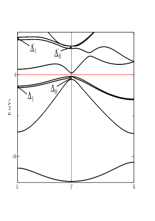
Figure 3: Band structure of GaAs calculated with the on-site approximation to the spin-orbit interaction.

We show in Fig. 3 the band-structure of the canonical III-V semiconductor, GaAs. The figure also defines graphically the energy splittings described in the previous paragraph. We note first that the band-structure closely resembles that obtained with other methodologies, and also agrees rather well with the experimental data,[38] except for the characteristic LDA underestimation of the semiconductor gap, which is further reduced because of the spin-orbit energy splitting. Therefore, in all the tests that follow, we have avoided narrow gap semiconductors, which are usually predicted to be metals by LDA.[36]

4.1 Band structure of Si

The spin-orbit energy splittings of silicon at the high symmetry points of the diamond lattice are presented in Table 1 and Fig. 4 for increasingly complete basis sets.

Basis	$E_{T}$ (eV)	$\Delta_{0}$ (eV)	$\Delta_{0}^{\prime}$ (eV)	$\Delta_{1}$ (eV)	$\Delta^{\prime}_{1}$ (eV)
SZ	-214.8	0.051	0.025	-	-
DZ	-215.0	0.068	0.157	0.027	0.105
TZ	-215.2	0.068	0.002	0.023	0.078
SZP	-215.8	0.042	0.787	0.024	0.032
DZP	-216.0	0.044	0.647	0.024	0.047
TZP	-216.0	0.045	0.696	0.025	0.050
TZDP	-216.0	0.045	0.604	0.026	0.043
TZTP	-216.0	0.045	0.593	0.026	0.044
TZTPF	-216.1	0.044	0.615	0.025	0.030
REF	-	0.044	0.04	0.02	0.03

Table 1: Spin-orbit energy splittings of bulk Si calculated for increasingly complete basis sets. $E_{T}$ is the total energy, $\Delta_{0}$, $\Delta_{0}^{\prime}$, $\Delta_{1}$ and $\Delta^{\prime}_{1}$ are the splittings as defined in the text. REF corresponds to the reference values, experimental whenever possible, as described in the literature.[38]

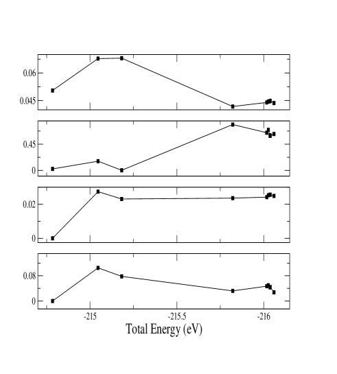
Figure 4: Convergence of the spin-orbit energy splittings of bulk Si with the size of the basis set. From top to bottom panels, we present respectively $\Delta_{0}$, $\Delta^{\prime}_{0}$, $\Delta_{1}$ and $\Delta^{\prime}_{1}$ as functions of the total energy associated with each set. The points correspond to SZ, DZ, TZ, SZP, DZP, TZP, TZDP, TZTP and TZTPF, respectively.

Our results are in extremely good agreement with the theoretical and experimental data available in the literature.[38] We note that a DZP basis set, which is usually assumed to be the minimal basis needed to obtain reasonably converged results, already provides accurate predictions for the energy splittings. The $\Delta^{\prime}_{0}$ split is somehow an anomaly, and in general we find that the splittings of the conduction bands are not as well described as those of the valence bands.

We note that Kohn-Sham eigenvalues should not be associated to single particle excitation energies, since the former are simply the Lagrangian multipliers leading to the Kohn-Sham equations. This is valid for both the valence and the conduction bands. However it is commonly accepted that DFT band structures are a good first approximation to single particle energies of occupied states. The conduction bands are somehow different since such states do not contribute to either the total energy and the density matrix, and therefore are irrelevant in DFT. For this reason a stark disagreement in the conduction band splitting should not be surprising. Moreover, the systematic overestimation of the $\Delta^{\prime}_{0}$ splitting is related to the underestimation of the bandgap. This produces an erroneous enhancement of the hybridisation between the orbitals forming the conduction bands with those forming the valence one, with a net overestimation of the spin-orbit splitting. It is therefore expected that corrective schemes to the bandgap may also correct the spin-orbit splitting of the conduction bands.

It is also important to note that basis where the radial component varies sharply around the origin should be avoided. These in fact are difficult to integrate in the range where the spin-orbit pseudopotential is appreciable and brings considerable numerical instability to the evaluation of the matrix elements.

Finally we have calculated the Si bulk parameters for different basis sets in order to check that the inclusion of spin-orbit interaction does not change significantly the LDA results. A summary of all the computed structural parameters is presented in Table 2.

Basis	$a$ (Å)	$BM$ (GPa)	$E_{c}$ (eV)
DZP	5.392	98.2	5.480
TZP	5.389	98.8	5.485
TZTP	5.388	98.2	5.491
PW	5.384	95.9	5.369
LAPW	5.41	96	5.28
EXP	5.43	98.8	4.64

Table 2: Structural parameters of bulk Si for several basis sets. $a$ is the lattice parameter, $BM$ the bulk modules and $E_{c}$ the cohesive energy. PW refers to a 50 Ryd cutoff plane-wave calculation.[34] LAPW corresponds to an all-electrons linear-augmented-plane-wave calculation[14] and EXP to the experimental values.[22]

4.2 III-V semiconductors

We have further tested our method by calculating the various energy splittings of several group IV and III-V semiconductors such as Ge, GaAs, AlAs and AlSb, i.e. of those with a reasonably large bandgap. For all of them we have found again that a DZP basis set provides essentially converged results. This is demonstrated in table 3 where we show that the splittings calculated with a DZP basis agree rather well with other theoretical estimates and with experimental values. Also in this case $\Delta_{0}^{\prime}$ is the exception for the same reasons explained before.

Material	$\Delta_{0}$ (eV)	$\Delta_{0}^{\prime}$ (eV)	$\Delta_{1}$ (eV)	$\Delta^{\prime}_{1}$ (eV)
Ge	0.2959	0.3783	0.1545	0.356
REF[4]	0.287	0.200	0.184	0.266
GaAs	0.3573	0.3006	0.1857	0.319
REF[38]	0.34	0.26	0.23	0.11
AlAs	0.3073	0.0762	0.1636	0.118
REF[26]	0.28	0.04	0.20	-
AlSb	0.6847	0.1752	0.3440	0.307
REF[38]	0.75	0.1	0.4	0.09

Table 3: Spin splittings for several III-V semiconductors as calculated with a DZP basis set. REF correspond to reference values, experimental whenever possible, as described in the literature.[4, 38, 26]

5 5d metals: Au and Pt

Since the spin-orbit interaction is a relativistic effect, it is expected to increase with the atomic number. Therefore, metals from the fifth row of the periodic table are an ideal test ground for our method. Among those, gold and platinum are specially good candidates, since the first is a closed-$d$ shell noble metal while the $d$-bands of the second have considerable weight at the Fermi energy. Moreover, a number of ab initio spin-orbit calculations are available [8] which demonstrate that the spin-orbit interaction is essential for the correct description of their band structures. To simulate these two materials, we have again used the LDA approximation for exchange and correlation potential, and constructed an optimised set consisting of two atomic wave functions in each of the s-, p- and d-channels.

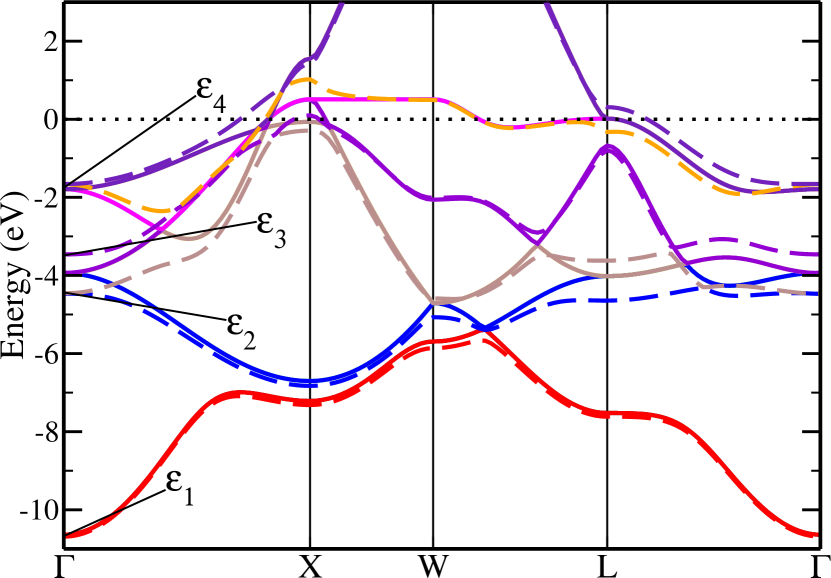
Figure 5: Band-structure of platinum obtained at the theoretical equilibrium lattice constant. The dashed line is for a spin-orbit calculation, while the solid line is obtained when the spin-orbit coupling is not included. The figure also provides a graphical definition of the energies at the $\Gamma$ point, $\varepsilon_{i}$, of the bands that are closest to the Fermi energy.

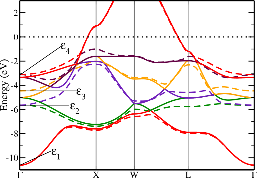
Figure 6: Band structure of gold obtained at the equilibrium theoretical lattice constant. The dashed line is for a spin-orbit calculation, while the solid line is obtained when the spin-orbit coupling is not included. The figure also provides a graphical definition of the energies at the $\Gamma$ point, $\varepsilon_{i}$, of the bands that are closest to the Fermi energy.

In Figs. 5 and 6 we present the band-structures of Pt and Au, calculated at the theoretical lattice constant, with and without taking into account the spin-orbit coupling. the figures show that s-bands are not modified by spin-orbit, while p- and d-bands suffer strong modifications, specially whenever two bands cross each other. Moreover, we find that the spin-orbit interaction lifts degeneracies at the band crossings as expected.

We summarise in Table 4 the bulk lattice constant and the energy of some selected bands at the $\Gamma$ point, that we define graphically in Fig. 5. These energies are in good agreement with other much more expensive methods, like Plane-wave pseudopotential (PWSCF)[8] and relativistic full-potential Korringa-Kohn-Rostoker (KKR)[37] methods or augmented plane-wave (APW) approaches for solving Dirac equation.[11] We note that the differences range in the order of only a few per cent.

Pt	SIESTA+On-site	PWSCF	KKR	APW
$a_{0}$ (Bohr)	7.45	7.40	7.36	7.414
$\varepsilon_{1}$(eV)	-10.53	-10.45	-10.56	-10.35
$\varepsilon_{2}$(eV)	-4.38	-4.38	-4.48	-4.24
$\varepsilon_{3}$(eV)	-3.38	-3.39	-3.47	-3.28
$\varepsilon_{4}$(eV)	-1.62	-1.53	-1.65	-1.48
Au	SIESTA+On-site	PWSCF	KKR	APW
$a_{0}$ (Bohr)	7.61	7.64	7.637	7.638
$\varepsilon_{1}$(eV)	-10.613	-10.18	-10.23	-9.95
$\varepsilon_{2}$(eV)	-5.645	-5.43	-5.41	-5.32
$\varepsilon_{3}$(eV)	-4.460	-4.23	-4.23	-4.14
$\varepsilon_{4}$(eV)	-3.111	-2.97	3.04	2.96

Table 4: Lattice constant and energy $\varepsilon_{i}$ of selected bands at $\Gamma$ point obtained with the use of the approximation presented in this article (SIESTA+On-site), and with PWSCF[8], KKR [37] and APW[11] methods. The definition of the energies $\varepsilon_{i}$ is provided in Figs. (3) and (4).

6 Conclusion

We have presented a simple and effective method for including the spin-orbit interaction in standard LCAO DFT calculations, which is based on relativistic norm-conserving pseudopotentials and on an on-site approximation to the spin-orbit matrix elements. The method is computational undemanding and extremely simple to implement in standard LCAO DFT codes, such as SIESTA. Importantly the on-site approximation does not introduce additional contributions to both forces and stress. We have then presented a series of tests for group IV and III-V semiconductors and for 5d metals. The overall structural parameters do not change with respect to standard non-relativistic LDA calculations, and are in general good agreement with reference data. The spin-orbit splittings of the band structures are also in good agreement with those obtained with more computationally intensive DFT methods.

The good results obtained for the electronic structures and structural parameters make our method very attractive for large scale simulations where spin-orbit coupling is relevant. This is for instance the case of semiconductors heterostructures and quantum-transport calculations [2] where spin-mixing effects are important.

References

References

- [1] Atomic units are used throughout the article.
- [2] Steve W. Bailey Alexandre R. Rocha, V ctor M. Garc a-Su rez, Colin J. Lambert, Jaime Ferrer, and Stefano Sanvito. Towards molecular spintronics. Nature Materials, 4(4):335–339, 2005.
- [3] Eduardo Anglada, José M. Soler, Javier Junquera, and Emilio Artacho. Systematic generation of finite-range atomic basis sets for linear-scaling calculations. Physical Review B, 66(205101):1–4, 2002.
- [4] D. E. Aspnes. Schottky-barrier electroreflectance of ge: Nondegenerate and orbitally degenerate critical points. Physical Review B (Solid State), 12(6):2297–2310, 1975.
- [5] Giovanni B. Bachelet and M. Schüter. Relativistic norm-conserving pseudopotentials. Physical Review B, 25(4):2103–2108, 1982.
- [6] P. Bruno. Electronic Structure: Basic Theory and Practical Methods. Cambridge University Press, Cambridge, 2004.
- [7] Till Burkert, Olle Eriksson, Peter James, Sergei I. Simak, Borje Johansson, and Lars Nordstrom. Calculation of uniaxial magnetic anisotropy energy of tetragonal and trigonal fe, co, and ni. Physical Review B (Condensed Matter and Materials Physics), 69(10):104426, 2004.
- [8] Andrea Dal Corso and Adriano Mosca Conte. Spin-orbit coupling with ultrasoft pseudopotentials: Application to au and pt. Physical Review B (Condensed Matter and Materials Physics), 71(11):115106, 2005.
- [9] M. J. Gillan D. R. Bowler, R. Choudhury and T. Miyazaki. Recent progress with large-scale ab initio calculations: the conquest code. Physica status solidi (b), 243(5):989–1000, 2006.
- [10] Supriyo Datta and Biswajit Das. Electronic analog of the electro-optic modulator. Applied Physics Letters, 56(7):665–667, 1990.
- [11] S. Bei der Kellen and A. J. Freeman. Self-consistent relativistic full-potential korringa-kohn-rostoker total-energy method and applications. Physical Review B (Condensed Matter), 54(16):11187–11198, 1996.
- [12] MJ Frisch et al. Gaussian 03, Revision C.02. Gaussian, Inc., Wallingford, CT, 2004.
- [13] R. P. Feynman. Forces in molecules. Physical Review, 56(4):340–343, 1939.
- [14] C. Filippi, D. J. Singh, and C. J. Umrigar. All-electron local-density and generalized-gradient calculations of the structural properties of semiconductors. Physical Review B, 50(20):14947–14951, 1994.
- [15] V M García-Suárez, C M Newman, C J Lambert, J M Pruneda, and J Ferrer. Optimized basis sets for the collinear and non-collinear phases of iron. Journal of Physics: Condensed Matter, 16(30):5453–5459, 2004.
- [16] Dante Gatteschi and Roberta Sessoli. Quantum tunneling of magnetization and related phenomena in molecular materials. Angew. Chem. Int. Ed., 42(3):268–297, 2003.
- [17] Stefan Goedecker. Linear scaling electronic structure methods. Reviews of Modern Physics, 71(4):1085–1123, 1999.
- [18] P. Hohenberg and W. Kohn. Inhomogeneous electron gas. Phys. Rev., 136(3B):B864–B871, Nov 1964.
- [19] Javier Junquera, Daniel Sánchez-Portal Óscar Paz, and Emilio Artacho. Numerical atomic orbitals for linear-scaling calculations. Physical Review B, 64(235111):1–9, 2001.
- [20] Y. K. Kato, R. C. Myers, A. C. Gossard, and D. D. Awschalom. Observation of the Spin Hall Effect in Semiconductors. Science, 306(5703):1910–1913, 2004.
- [21] J. M. Kikkawa and D. D. Awschalom. Lateral drag of spin coherence in gallium arsenide. Nature, 397(6715):139–141, 1999.
- [22] C. Kittel. Introduction to Solid State Physics. Wiley, New York, 1986.
- [23] Leonard Kleinman. Relativistic norm-conserving pseudopotential. Physical Review B, 21(6):2630–2631, 1980.
- [24] Leonard Kleinman and D. M. Bylander. Efficacious form for model pseudopotentials. Physical Review Letters, 48(20):1425–1428, 1982.
- [25] W. Kohn and L. J. Sham. Self-consistent equations including exchange and correlation effects. Phys. Rev., 140(4A):A1133–A1138, Nov 1965.
- [26] Kurt A. Mäder and Alex Zunger. Empirical atomic pseudopotentials for alas/gaas superlattices, alloys, and nanostructures. Phys. Rev. B, 50(23):17393–17405, Dec 1994.
- [27] Richard M. Martin. Electronic Structure: Basic Theory and Practical Methods. Cambridge University Press, Cambridge, 2004.
- [28] Marco H ser an Hans Horn Reinhart Ahlrichs, Michael B r and Christoph K lmel. Electronic structure calculations on workstation computers: The program system turbomole. Chemical Physics Letters, 162(3):165–169, 1989.
- [29] L. M. Sandratskii. Noncollinear magnetism in itinerant-electron systems: theory and applications. Adv. Phys., 47(1):91–160, 1998.
- [30] Otto F. Sankey and David J. Niklewski. Ab initio multicenter tight-binding model for molecular-dynamics simulations and other applications in covalent systems. Physical Review B (Condensed Matter), 40(6):3979–3995, 1989.
- [31] F. Schwabl. Quantum Mechanics. Springer, Berlin, 2002.
- [32] Spencer D. Shellman, James P. Lewis, Kurt R. Glaesemann, Krzysztof Sikorski, and Gregory A. Voth. Massively parallel linear-scaling algorithm in an ab initio local-orbital total-energy method. J. Comput. Phys., 188(1):1–15, 2003.
- [33] Chris-Kriton Skylaris, Peter D Haynes, Arash A Mostofi, and Mike C Payne. Using onetep for accurate and efficient density functional calculations. Journal of Physics: Condensed Matter, 17(37):5757–5769, 2005.
- [34] José M. Soler, Emilio Artacho, Julian D. Gale, Alberto Garcia Javier Junquera, Pablo Ordejón, and Daniel Sánchez-Portal. The SIESTA method for ab initio order-N materials simulations. Journal of Physics: Condensed Matter, 14:2745–2779, 2002.
- [35] Nicola A. Hill Stefano Sanvito, Gerhard Theurich. Density Functional Calculations for III-V Diluted Ferromagnetic Semiconductors: A Review. Journal of Superconductivity, 15(1):85–104, 2002.
- [36] Michael P. Surh, Ming-Fu Li, and Steven G. Louie. Spin-orbit splitting of GaAs and InSb bands near . Physical Review B, 43(5):4286–4294, 1991.
- [37] V. Theileis and H. Bross. Relativistic modified augmented plane wave method and its application to the electronic structure of gold and platinum. Physical Review B (Condensed Matter and Materials Physics), 62(20):13338–13346, 2000.
- [38] G. G. Wepfer, T. C. Collins, and R. N. Euwema. Calculated spin-orbit splittings of some group iv, iii-v, and ii-vi semiconductors. Physical Review B (Solid State), 4(4):1296–1306, 1971.
- [39] S. A. Wolf, D. D. Awschalom, R. A. Buhrman, J. M. Daughton, S. von Molnar, M. L. Roukes, A. Y. Chtchelkanova, and D. M. Treger. Spintronics: A Spin-Based Electronics Vision for the Future. Science, 294(5546):1488–1495, 2001.
- [40] P. Y. Yu and M. Cardona. Fundamentals of Semiconductors: Physics and Materials Properties. Berlin: Springer, 2005.