Fluorescence Intermittency of A Single Quantum System and Anderson Localization

Abstract

The nature of fluorescence intermittency for semiconductor quantum dots (QD) and single molecules (SM) is discussed from the viewpoint of Anderson localization. The power law distribution for the on time is explained as due to the interaction between QD/SM with a random environment. In particular, we find that the on-time probability distribution behaves differently in the localized and delocalized regimes. They, when properly scaled, are universal for different QD/SM systems. The on-time probability distribution function in the delocalized QD/SM regime can be approximated by power laws with exponents covering $-2\leq m<0$.

Recent development in nano-fabrication and measurement has made it possible to probe directly the dynamics of a single quantum system and its coupling with local environment. For optical measurements, in particular, fluorescence intermittency (FI) occurs in a wide class of single quantum systems including semiconductor nanocrystals KFHGN ; SNLEWB ; VOO ; CMB ; IBC and single molecules SCB1 ; SCB2 ; SCB3 . This optical phenomenon is experimentally found to be a robust and fundamental property of single photon emitters. The random switching between an emitting (on) and a non-emitting (off) state is characterized by on-time and off-time distribution functions. Surprisingly, the distribution functions can often be fitted by power laws instead of exponentials. The exponents of the power laws vary from system to system and they are almost independent of temperature. To explain this unusual behavior, Marcus et. al. TM1 ; FM recently proposed a model based on diffusion in energy space. An exponent of $-1.5$ is readily obtained for one-dimensional diffusion processes. Deviation from $-1.5$ is explained by anomalous diffusion, which has its origin from the Cole-Davison dielectric medium $\beta\neq 1$. However, this scenario would predict exponents that are temperature dependent. Recent experiments also found that exponents $\sim-2.0$ for the on time exist in many different single emitters KFHGN ; CMB ; SCB1 ; SCB2 ; SCB3 , which are imbedded in various media. The temperature-independence of power laws with $m_{\text{on/off}}\neq-1.5$ and robustness of $m_{\text{on}}=-2.0$ need to be explained.

In this work, we provide a microscopic Hamiltonian model which does not build on the assumption of anomalous diffusion in energy space and the quadratic form of diffusion potential. The purpose of this work is to lay the foundation for a quantum-mechanical theory of FI. In a classic paper A , Anderson considered a transport process which involves solely quantum-mechanical motion in a random lattice. His quantum-mechanical treatment of the process leads to the concept of Anderson localization, which has been applied extensively to the problem of transport in a random environment. Here, we view the blinking as a charge hopping process between the QD/SM and the traps in the environment. We find that the FI can be explained in the framework of the Anderson localization. The basic idea is the following: due to the coupling to a random environment, the on-site energy of a QD/SM is renormalized and becomes a random variable. In addition, random configurations of the local environment lead to a distribution of decaying (hopping) rates for the QD/SM. This is the physical origin of the on-time distribution.

Based on experimental results, we study the following simple tight-binding Hamiltonian:

$$\hat{H}=\varepsilon_{d}\hat{d}^{\dagger}\hat{d}+\sum_{j}\varepsilon_{j}\hat{c}_{j}^{\dagger}\hat{c}_{j}+\sum_{j}v_{j}\left(\hat{d}^{\dagger}\hat{c}_{j}+\hat{c}^{\dagger}_{j}\hat{d}\right)$$ (1)

The ground state is defined such that the QD/SM is neutral. For a QD this corresponds to a filled valence band. When an electron is excited by photon to an excited state, it relaxes to the lowest excited state on a time scale from hundreds of femtoseconds to picoseconds. This lowest excited state is responsible for photon emission and hopping to traps in the matrix. This state could be $1S$ state for QDs and it may involve some surface states as well KSMLB ; KMMLB . The excited electron completes a radiative cycle on a time scale of the order inverse Rabi frequency: $\Omega^{-1}_{\text{Rabi}}$. This time scale is much smaller than the typical bin size, $\geq$0.2 ms, used in the experiments. Since the excited electronic state is near resonance with the ground state plus a photon, we define the on-state as the following: it is a dressed electronic state NOTE1 which has the same bare energy as the excited electronic state, $\varepsilon_{d}$, but with an infinite lifetime when it is decoupled from the trap states. Physically, this means that when there is no coupling to the environment, the excited electron localizes inside the QD/SM and the QD/SM, being in the on-state, keeps emitting photons. Such an on-state is created by operator $\hat{d}^{\dagger}$. The bare on-site energy $\varepsilon_{d}$ is renormalized due to interaction with trap sites $j$. The coupling constant is $v_{j}$. The trap site $j$ is created by operator $\hat{c}^{\dagger}_{j}$ and has a random energy $\varepsilon_{j}$. Here we focus on the class of random environments that are formed by topologically random network of chemical bonds. Randomness could arise from a spatially fluctuating potential due to charged impurities and coupling with phonons that arise from deformation of a random lattice. The details of randomness are irrelevant to the dynamical response of the system as is known from scaling theory of localization. For simplicity, we assume all traps follow the same energy distribution function $p(\varepsilon)$.

Mathematically, the above definitions are equivalent to defining the zeroth order Green’s function of the on-state as: $G^{(0)}_{d}(\omega)=\frac{1}{\omega-\omega_{d}+i\eta}$, with $\omega_{d}=\varepsilon_{d}/\hbar$, and $\eta$ being an infinitesimally small and positive constant. Similarly, the zeroth order Green’s functions of the traps are $G^{(0)}_{j}(\omega)=\frac{1}{\omega-\omega_{j}+i\eta}$. The decay rate of the on-state can be calculated from the full Green’s function $G_{d}(\omega)=\frac{1}{\omega-\omega_{d}-\Sigma_{s}(\omega)}$ where the only self-energy of the model is

$$\Sigma_{s}(\omega)=\frac{1}{\hbar^{2}}\sum_{j}\frac{v_{j}^{2}}{\omega-\omega_{j}+i\eta}$$ (2)

One obtains the renormalized energy and decay rate from the pole equation. The results to $O(v_{j}^{2})$ are:

$$E_{d}=\varepsilon_{d}+\sum_{j}\frac{v_{j}^{2}(\varepsilon_{d}-\varepsilon_{j})}{(\varepsilon_{d}-\varepsilon_{j})^{2}+\eta^{2}}$$ (3a)

$$\Gamma=\sum_{j}\frac{2v_{j}^{2}}{\hbar}\frac{\eta}{(\varepsilon_{d}-\varepsilon_{j})^{2}+\eta^{2}}$$ (3b)

Since each $\varepsilon_{j}$ is a random variable, both the renormalized energy $E_{d}$ and decay rate $\Gamma$ are random variables. Physically, this corresponds to the situation in which environment stays at a certain configuration for a period of time during which a physical decay rate can be defined. The ensemble of configurations that the environment takes on gives rise to a distribution of decay rates. This picture is valid when static disorder dominates or when the environment is ergodic.

To find the decay rate distribution function, $f(\Gamma)$, from $p(\varepsilon_{j})$, one must perform a summation over random variables $\varepsilon_{j}$. In addition, due to lattice deformation, a random spatial distribution of traps must also be assumed. For simplicity, we assume that all the traps follow the same distribution function $\rho(\textbf{r})$. We will consider two physical regimes, namely the delocalized and the localized regimes, for the excited electron on the QD/SM according to the framework of Anderson A .

The delocalized regime corresponds to most of the experimentally studied situations. Essentially, electrons excited inside the QD/SM can make real transitions to the trap sites in the matrix through the mechanism of quantum tunneling, and then become localized. When this happens, the QD/SM becomes ionized. The results in this regime, which will be shown later, support the random resonance picture: on average, the energy of a QD/SM, is far off-resonance with trap energies, i.e. $\varepsilon_{d}\gg\varepsilon_{j}$. The electrons of QD/SM remain localized (on state) until a random fluctuation of $\varepsilon_{j}$ makes it on-resonance with the QD/SM. This random resonance could be realized through interaction with phonons MA . Since there is finite probability that $\varepsilon_{d}-\varepsilon_{j}\sim\eta\sim 0^{+}$, one cannot perform the summations in the same way as in A . Instead, nontrivial summations of the whole expression (3b) are required. The distribution function $f(\Gamma)$ can be calculated by method of Fourier transformation:

$$f(\Gamma)=\int_{-\infty}^{\infty}\frac{dt}{2\pi}~{}\psi(t)~{}e^{-i\Gamma t}$$ (4)

The Fourier transformed probability distribution function $\psi(t)$ is given by

$$\psi(t) = \int_{-\infty}^{\infty}\prod_{j=1}^{N}d\varepsilon_{j}p(\varepsilon_{j})\exp\left[it\sum_{k=1}^{N}\frac{2v_{k}^{2}}{\hbar}\frac{\eta}{(\varepsilon_{d}-\varepsilon_{k})^{2}+\eta^{2}}\right]$$ (5)

$$= \exp\left\{N\ln\mathcal{I}\right\}$$

where $N$ is the number of traps and

$$\mathcal{I}=\int_{-\infty}^{\infty}d\varepsilon\int d\textbf{r}~{}p(\varepsilon)\rho(\textbf{r})\exp\left[i\frac{2tv(\textbf{r})^{2}}{\hbar}\frac{\eta}{(\varepsilon_{d}-\varepsilon)^{2}+\eta^{2}}\right]$$

The integral $\mathcal{I}$ is obtained under the assumptions made above, i.e. identical energy and spatial distributions of traps. This integral needs to be done carefully so that we can express it in powers of $\eta$. For a real physical system coupled to a disordered environment, $\eta$ is small but nonetheless not strictly zero. Physically, this is due to competing non-radiative relaxation channels which contribute to a small but finite width of resonance. The value of $\eta$ can be calculated in a more sophisticated model, however, in our model we take it as a fitting parameter. Changing variable to the dimensionless $u=\frac{\hbar}{2\pi v(\textbf{r})^{2}|t|}\varepsilon$ and noticing $\frac{1}{\pi}\frac{\eta}{(u-u_{d})^{2}+\eta^{2}}$ can be approximated by an impulse function centered at $u=u_{d}$ as $\eta$ is sufficiently small, where $u_{d}=\frac{\hbar}{2\pi v(\textbf{r})^{2}|t|}\varepsilon_{d}$, we can separate the integral into three parts: $(-\infty,u_{d}-\eta/2]$, $(u_{d}-\eta/2,u_{d}+\eta/2)$ and $[u_{d}+\eta/2,+\infty)$ to obtain the expansion:

$$\mathcal{I}=1-\eta\left[1-\cos\left(\frac{1}{\eta}\right)-i~{}\text{sign}(t)\sin\left(\frac{1}{\eta}\right)\right]p(\varepsilon_{d})\frac{2\pi}{\hbar}\langle v(\textbf{r})^{2}\rangle|t|+O(\eta^{3})$$

Since we are interested in case where there are a large number of traps $N\gg 1$, by substituting the expansion to Eq.(5) we rewrite the unknown parameter $N\eta$ as $N\eta=a_{0}n$ A ; NOTE2 , where $n$ is the density of traps and $a_{0}$ is a fitting parameter. Absorbing the numerical constant in the square bracket of $\mathcal{I}$ into $a_{0}$ and neglecting an unimportant imaginary part as is justified in this delocalized regime, we get

$$\psi(t)=\exp\left\{-\frac{2\pi}{\hbar}\langle v(\textbf{r})^{2}\rangle p(\varepsilon_{d})na_{0}|t|\right\}$$ (6)

The probability distribution function $f(\Gamma)$ in the delocalized QD/SM regime:

$$f(\Gamma)=\frac{1}{\pi}\frac{\Gamma_{0}}{\Gamma^{2}+\Gamma_{0}^{2}}$$ (7)

is Lorentzian, with the characteristic decay rate $\Gamma_{0}$ given by:

$$\Gamma_{0}=\frac{2\pi}{\hbar}\langle v(\textbf{r})^{2}\rangle p(\varepsilon_{d})na_{0}$$ (8)

The on-time distribution function can be calculated as $P_{\text{on}}(t)=\int_{0}^{\infty}d\Gamma\exp(-\Gamma t)f(\Gamma)$ which turns out to be:

$$P_{\text{on}}(t)=-\frac{2\Gamma_{0}}{\pi}\left[\cos(\Gamma_{0}t)\text{ci}(\Gamma_{0}t)+\sin(\Gamma_{0}t)\text{si}(\Gamma_{0}t)\right]$$ (9)

where ci and si are cosine and sine integrals GR respectively.

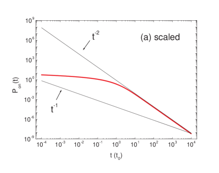
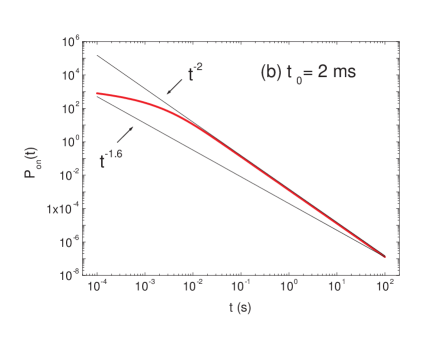
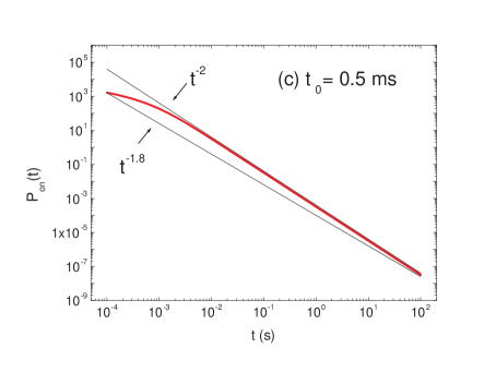
Figure 1: Probability distribution functions for the on time in the delocalized regime. (a) Universal on-time probability distribution function obtained by scaling in a characteristic on-state lifetime $t_{0}=1/\Gamma_{0}$. (b) $P_{\text{on}}(t)$ for a QD/SM with a lifetime $2\text{ms}$ and a fixed observation window. The exponents of the fitting power laws lie between $-1.6$ and $-2$. (c) $P_{\text{on}}(t)$ of a QD/SM with a shorter lifetime $0.5\text{ms}$. The exponents of the fitting power laws lie between $-1.8$ and $-2$.

The expression for $P_{\text{on}}(t)$ in (9) has several physical implications. First of all, it depends only on one parameter $\Gamma_{0}$ (this is also true for $P_{\text{on}}(t)$ in the localized regime (12), which only depends on the parameter $\gamma_{0}$). The characteristic decay rate $\Gamma_{0}$, is purely due to quantum tunneling and depends on the degree of disorder $p(\varepsilon_{d})\langle v(\textbf{r})^{2}\rangle$. This is a generic feature of Anderson localization theory. Only the energy fluctuation of traps evaluated at the bare QD/SM on-site energy, $p(\varepsilon_{d})$, comes into the final result. This supports the random resonance picture discussed above. The one-parameter theory also implies that experimental results for different QD/SM systems, when plotted in unit of characteristic on-time lifetime $t_{0}=1/\Gamma_{0}$, follow a universal distribution Fig.1(a). In the long time limit, $t\gg t_{0}$, $P_{\text{on}}(t)\sim t^{-2}$. The exponent of $-2$ comes from the peak of the Lorentzian distribution for decay rates, which physically indicates the resonant scattering condition. This $-2$ exponent is also robust and it does not depend on the properties of matrix or emitters SCB1 . In experiments, the observation time is fixed so that one probes only a certain range ($3$ to $4$ orders of magnitude in physical time) of the whole probability distribution. The location of the window in the universal distribution depends on $\Gamma_{0}$, which is not universal. If one fits the experimental data with power laws, then the exponents of the power laws will implicitly depend on $\Gamma_{0}$ except for the $m_{\text{on}}=-2$ case. From (8) we see that $\Gamma_{0}$ depends on properties of the QD/SM and its embedding matrix. This is one major difference between our theory and the diffusion-controlled electron transfer theory TM1 for the on-time statistics. In the latter, the exponents of the fitting power laws come from properties of the dielectric medium alone, i.e. the $\beta$ parameter of the Cole-Davison equation, which depends on temperature. As $\Gamma_{0}$ rises with increasing coupling strength between the QD/SM and its local environment, power law exponents observed for SMs would in principle larger than (in absolute value) that of well-coated QDs. This is indeed consistent with current experimental resultsSNLEWB ; SCB1 .

The quantum mechanical theory of FI allows a weak temperature-dependence of the on-time probability density. This comes from the fact that the energy fluctuation of trap sites, besides the mechanisms discussed above, has a temperature component. This dependence is usually very weak since the typical energy difference between $\varepsilon_{d}$ and $\varepsilon_{j}$ is on the order of $1\sim 2$ eV which is much larger than the magnitude of thermal broadening around $\varepsilon_{j}$. Increasing temperature slightly increases $p(\varepsilon_{d})$ since $\varepsilon_{d}\gg\varepsilon_{j}$ and as a result $\Gamma_{0}$ increases. So higher temperature would slightly decrease $m_{\text{on}}$ towards $-2$ for the long time.

In the case that the excited QD/SM electron is localized, then we predict very long on times. This corresponds to the off-resonance situation, $\varepsilon_{d}-\varepsilon_{j}\gg\eta,\forall j$. One can calculate the probability distribution of $\Gamma=\frac{2\eta}{\hbar}\sum_{j}\frac{v_{j}^{2}}{(\varepsilon_{d}-\varepsilon_{j})^{2}}$, using the results of A :

$$f(\Gamma)=\gamma_{0}^{\frac{1}{2}}\Gamma^{-\frac{3}{2}}\exp\left(-\pi\gamma_{0}/\Gamma\right)$$ (10)

where the characteristic decay rate $\gamma_{0}$ is

$$\gamma_{0}=\frac{2\eta}{\hbar}\left[\frac{a_{0}n\langle v(\textbf{r})\rangle}{W}\right]^{2}$$ (11)

$W$ is the width of energy fluctuation for the traps. $n$ is the density of traps, while $a_{0}\sim O(1)$ is a constant with a dimension of volume. Note that in the limit $\eta\rightarrow 0$, then $\gamma_{0}\rightarrow 0$ and the probability distribution function of decay rates is only nonzero when $\Gamma=0$, i. e. the QD/SM electron is localized. Physically, the smallness of $\eta$ has to be compared with the energy difference $\epsilon_{d}-\epsilon_{j}$ AGD . As discussed in the delocalized regime, the coupling of trap electrons with phonons and non-radiative processes etc. can lead to a sufficiently small, but non-zero value of $\eta$. The above results are applicable to many topologically disordered systems LW . Thus, for a QD/SM in this regime, the single emitter experiences very long bright periods, which are characterized by $1/\gamma_{0}$. The on-time probability distribution function is obtained from (10):

$$P_{\text{on}}(t)=\left(\frac{t}{\pi\gamma_{0}}\right)^{-\frac{1}{2}}\exp\left(-\sqrt{4\pi\gamma_{0}t}\right)$$ (12)

So in the limit $t\ll 1/\gamma_{0}$, the probability distribution of the on-time follows a power law with an exponent of $-1/2$. On a much longer time scale, $P_{\text{on}}(t)$ deviates from the power law and shows a stretched-exponential tail. This stretched-exponential tail is of purely quantum nature and depends on the degree of disorder $W/\langle v(\text{r})\rangle$.

Now we discuss the mechanism for the off-time probability distribution. Suppose a charge is on the trap site $j$. The self-energy of $G_{j}(\omega)$ is $G_{d}(\omega)$. The decay rate is vanishingly small, so the charge is localized. Then on-state can only be recovered via quantum tunnelling of trapped electrons. $P_{\text{off}}(t)$ is therefore given by

$$P_{\text{off}}(t)=\int_{0}^{\infty}drg(r)\gamma_{\text{off}}(r)\exp\left[-\gamma_{\text{off}}(r)t\right]$$ (13)

where $g(r)$ is the probability density of an excited electron having been trapped at a distance of $r$ from the QD/SM and it is proportional to the square of the excited state wave function. $\gamma_{\text{off}}(r)$ is the decay rate of a trapped electron to the QD/SM. A model based on this picture was first proposed by Verberk et.al. VOO and experimentally examined in IBC . Since the typical size of a QD/SM is of the order $30$Å in radius, so to a good approximation, the QD/SM can be viewed as a shallow impurity K and one can use effective mass theory. The wave function of an excited QD/SM electron behaves as $\exp(-r/a)$ at large distances, where $a=\hbar^{2}\epsilon_{0}\kappa/m^{\ast}_{d}e^{2}=\tilde{a}\kappa$ is the effective Bohr radius and is related to the ionization energy, $E_{\text{ion}}$, of the excited electron by $a=\hbar/\sqrt{2m^{\ast}_{d}E_{\text{ion}}}$. $\kappa$ is the relative static dielectric constants of the media. $m^{\ast}_{d}$ is the effective mass of the QD/SM electron. Similarly, $\gamma_{\text{off}}(r)$ is given by MA : $\gamma_{\text{off}}\exp(-2r/b)$, where $b=\hbar/\sqrt{2m^{\ast}_{t}E_{t}}$ is the spatial extent of a trapped electron’s wave function with $m^{\ast}_{t}$ and $E_{t}$ being the effective mass and ionization energy at the trap site. We obtain $P_{\text{off}}(t)\approx Ct^{-m_{\text{off}}}$ with $C=a\Gamma(1+b/a)/\gamma_{\text{off}}^{b/a}b$ and

$$m_{\text{off}}=1+\frac{b}{a}=1+\sqrt{\frac{m^{\ast}_{d}E_{\text{ion}}}{m^{\ast}_{t}E_{t}}}=1+\frac{b}{\tilde{a}}\frac{1}{\kappa}$$ (14)

We see that the difference in $m_{\text{off}}$ for different systems comes mainly from the effective mass $m^{\ast}_{d}$ and the ability of a matrix to stabilize the charged QD/SM and the ejected electron. In contrast to the diffusion model TM1 , the exponents of $P_{\text{off}}(t)$ depend on the relative static dielectric constant $\kappa$ instead of the Cole-Davison $\beta$ parameter. This is consistent with recent experimental results SCB1 ; IBC . In addition, our model allows $m_{\text{off}}$ to take a different value from $m_{\text{on}}$ KFHGN ; CMB ; SCB1 ; SCB2 , while the diffusion model predicts that they must be the same.

To conclude, we have proposed a mechanism for FI as being a manifestation of Anderson localization. The on-time manifold is shown to be generated by different realizations of electron delocalization from the QD/SM through the mechanism of random resonance. The quantum theory predicts a universal probability distribution function for the on time and shows $m_{\text{on}}=-2$ is indeed a robust result, which corresponds to the long time limit of $P_{\text{on}}(t)$. The off state corresponds to a localized electron in the environment. The recovery of the on state is realized via quantum tunneling.

This work is supported by the National Science Foundation (NSF) under the Grant No. CHE0306287.

References

- (1) M. Kuno, D. P. Fromm, H. F. Hamann, A. Gallagher, and D. J. Nesbitt, J. Chem. Phys. 115(2), 1028(2001)
- (2) K. T. Shimizu, R. G. Neuhauser, C. A. Leatherdale, S. A. Empedocles, W. K. Woo, and M. G. Bawendi, Phys. Rev. B 63, 205316(2001)
- (3) R. Verberk, A. M. van Oijen, and M. Orrit, Phys. Rev. B 66, 233202(2002)
- (4) F. Cichos, J. Martin and C. von Borczyskowski, Phys. Rev. B 70, 115314 (2004)
- (5) A. Issac, C. von Borczyskowski and F. Cichos, Phys. Rev. B 71, 161302(R) (2005)
- (6) J. Schuster, F. Cichos and C. von Borczyskowski, Appl. Phys. Lett. 87, 051915(2005)
- (7) J. Schuster, F. Cichos and C. von Borczyskowski, Opt. Spectrosc. 98, 712(2005)
- (8) J. Schuster, F. Cichos and C. von Borczyskowski, to be published
- (9) J. Tang and R. A. Marcus, Phys. Rev. Lett. 95, 107401(2005)
- (10) P. A. Frantsuzov and R. A. Marcus, Phys. Rev. B 72, 155321(2005)
- (11) P. W. Anderson, Phys. Rev. 109, 1492(1958)
- (12) V. I. Klimov, Ch. J. Schwarz, D. W. McBranch, C. A. Leatherdale and M. G. Bawendi, Phys. Rev. B 60, R2177(1999)
- (13) V. I. Klimov, A. A. Mikhailovsky, D. W. McBranch, C. A. Leatherdale and M. G. Bawendi, Phys. Rev. B 61, R13349(2000)
- (14) The dressed electronic state is a linear superposition of and .
- (15) A. A. Abrikosov, L. P. Gorkov, and I. E. Dzyaloshinski, Methods of Quantum Field Theory in Statistical Physics (Pergamon, Elmsford, N.Y., 1965)
- (16) D. E. Logan and P. G. Wolynes, Phys. Rev. B 36, 4135(1987)
- (17) A. Miller and E. Abrahams, Phys. Rev. 120, 745(1960)
- (18) In the case when translational symmetry is preserved, this corresponds to the conventional treatment of changing summation to an integration weighted by energy density of states and thus gives finite .
- (19) I. S. Gradshteyn and I. M. Ryzhik, Table of Integrals, Series and Products, 6th Edit.(Academic Press, 2000)
- (20) W. Kohn, Solid State Physics, vol. 5 edited by F. Seitz and D. Turnbull (Academic Press, New York, 1957)