Synchronization Landscapes in Small-World-Connected Computer Networks

Abstract

Motivated by a synchronization problem in distributed computing we studied a simple growth model on regular and small-world networks, embedded in one and two-dimensions. We find that the synchronization landscape (corresponding to the progress of the individual processors) exhibits Kardar-Parisi-Zhang-like kinetic roughening on regular networks with short-range communication links. Although the processors, on average, progress at a nonzero rate, their spread (the width of the synchronization landscape) diverges with the number of nodes (desynchronized state) hindering efficient data management. When random communication links are added on top of the one and two-dimensional regular networks (resulting in a small-world network), large fluctuations in the synchronization landscape are suppressed and the width approaches a finite value in the large system-size limit (synchronized state). In the resulting synchronization scheme, the processors make close-to-uniform progress with a nonzero rate without global intervention. We obtain our results by “simulating the simulations”, based on the exact algorithmic rules, supported by coarse-grained arguments.

I Introduction

The study of complex networks pervades various areas of science ranging from sociology to statistical physics ALBERT02 ; DOROGOVTSEV02 ; NEWMAN03 . A network in terms of modeling can be defined as a set of items, referred to as nodes with links connecting them. Examples of real life complex networks include the Internet FALOUTSOS99 ; BARABASI99 , the World Wide Web ALBERT99 , metabolic networks JEONG00 , transportation networks VESPIG2004 ; AMARAL2005 , and social networks EUBANK04 .

Regular lattices are commonly used to study physical systems with short-range or long-range interactions. Earlier network studies focused mostly on the topological properties of the networks. Recent works, motivated by a large number of natural and artificial systems, such as the ones listed above, have turned the focus onto processes on networks, where the interaction and dynamics between the nodes are facilitated by a complex network. The question then is how the collective behavior of the system is influenced by this possibly complex interaction topology. Watts and Strogatz, inspired by a sociological experiment MILGRAM67 , have proposed a network model known as the small-world (SW) network WATTS98 . The SW concept describes the observation that, despite their often large size, there is a relatively short path between any two nodes in most networks with some degree of randomness. The SW model was originally constructed as a network to interpolate between regular lattices and completely random networks ERDOS60 . Systems and models (with well known behaviors on regular lattices) have been studied on SW networks, such as the Ising model SCALETT91 ; GITTERMAN00 ; BARRAT00 ; Wheeler , the XY model KIM01 , phase ordering HONG02_2 , the Edwards-Wilkinson model KOZMA03 ; KOZMA05 ; KOZMA05b , diffusion MONASSON99 ; BLUMEN_2000a ; BLUMEN_2000b ; ALMAAS_2002 ; KOZMA03 ; KOZMA05 ; KOZMA05b ; HASTINGS04 , and resistor networks KORN_PLA_swrn . Closely related to phase transitions and collective phenomena is synchronization in coupled multi-component systems WIESENFELD96 . SW networks have been shown to facilitate autonomous synchronization which is an important feature of these networks from both fundamental and system-design points of view STROGATZ01 ; BARAHONA02 ; HONG02_1 . In this paper we study a synchronization problem which emerges KORN00_PRL in certain parallel distributed algorithms referred to as parallel discrete-event simulation (PDES) FUJIMOTO90 ; NICOL94 ; LUBA00 ; KOLA_REV_2005 . First, we find that constructing a SW-like synchronization network for PDES can have a strong impact on the scalability of the algorithm KORN03_SCI . Secondly, since the particular problem is effectively “local” relaxation in a noisy environment in a SW network, our study also contributes to the understanding of collective phenomena on these networks.

Simulation of large spatially extended complex systems in physics, engineering, computer science, or military applications require vast amount of CPU-time on serial machines using sequential algorithms. PDES enabled researchers to implement faithful simulations on parallel/distributed computer systems, namely, systems composed of multiple interconnected computers FUJIMOTO90 ; NICOL94 ; LUBA00 ; KOLA_REV_2005 . PDES is a subclass of parallel and distributed simulations in which changes in the components of the system occur instantaneously from one state to another. These changes are referred to as discrete events, e.g., spin-flip attempts in magnetic Ising models with Glauber dynamics. The primary motivation in PDES is to perform parallel simulation for large systems without altering the original physical dynamics. In the physics, chemistry and biology communities these types of simulations are most commonly referred to as dynamic or kinetic Monte Carlo simulations. Examples for real-life complex systems where discrete-event models are applicable include cellular communication networks LUBA00 ; GREEN94 , magnetic systems KORN99_JCP ; KORN01_PRE , spatial epidemic models EUBANK04 ; DEEL96 , thin-film growth AMAR_PRB_2005a ; AMAR_PRB_2005b ; AMAR_JCP_2005 , battle-field models NICOL88 , and internet traffic models COWIE99 . In the above examples the discrete events are call arrivals, spin-flip attempts, infections, monomer depositions, troop movements, and packet transmissions/receptions respectively.

PDES has two basic ingredients: the set of local simulated times of the processors or processing elements (PE) (also referred to as virtual times JEFF85 ) and a synchronization scheme FUJIMOTO90 . The difficulty in PDES is that the discrete events are not synchronized by a global clock since the dynamic is usually asynchronous. The challenge is algorithmically parallelizing the physically non-parallel dynamics, while enforcing causality between events and reproducibility. There are two main approaches in PDES: (i) conservative synchronization, which avoids the possibility of any type of causality errors by checking the causality relation between potentially related events at every update attempt CHANDY79 ; CHANDY81 and (ii) optimistic synchronization, which allows possible causality errors, then later initiates rollbacks to correct the erroneous computations JEFF85 ; DEELMAN97 . Innovative methods have also been introduced to make optimistic synchronization more efficient, such as reverse computation CAROTHERS99 . Other recent improvements to exploit parallelism in discrete-event systems are the “lookback” method CHEN02 and the freeze-and-shift algorithm SHCHUR04 .

As the number of available PEs on parallel architectures increases to tens of thousands TOP500_IBM , and high-performance grid-computing networks emerge GRID ; KIRKPATRICK03 , fundamental questions of the scalability of the underlying algorithms must be addressed. A PDES should have the following properties to be scalable GREEN94 : (i) the virtual time horizon formed by the virtual times of the PEs should progress on average with a non-zero rate and (ii) the typical spread (width) of the time horizon should be bounded as the number of PEs, $N_{PE}$, goes to infinity. The latter condition becomes important to avoid long delays while waiting for “slow” nodes AMAR_PRB_2005a or, alternatively, to eliminate the need to reserve a large amount of memory for temporary data storage. In this paper we study regular and SW network communication topologies and show a possible way to construct fully scalable parallel algorithms for systems with asynchronous dynamics and short-range interactions on regular lattices.

In order to understand scalability and synchronizability of PDES, we consider the parallel simulation itself as a complex interacting system where the specific synchronization rules correspond to the “microscopic dynamics”. A similar approach was also successful to establish a connection SLOOT01 between rollback-based (or optimistic) schemes JEFF85 and self-organized criticality BAK87 ; BAK88 . Our approach exploits a mapping between non-equilibrium surface growth and the evolution of the simulated time horizon KORN00_PRL ; KORN00_UGA so that we can use the tools and framework of statistical mechanics. A similar analogy between phase transitions and computational complexity has turned out to be highly fruitful to gain more insight into traditional hard computational problems COMPLEX ; MONA99 . In this paper we consider the scalability of conservative synchronization schemes for self-initiating processes NICOL91 ; FELDER91 , where update attempts on each node are modeled as independent Poisson streams. We study the morphological properties of the simulated time horizon (or synchronization landscape). Through our study one also gains some insight into the effects of SW-like interaction topologies on the critical fluctuations in interacting systems.

This paper, in part, is an expanded version of our earlier works on one-dimensional (1D) KORN00_PRL and 1D SW (SW embedded in one dimension) synchronization networks KORN03_SCI . Further, we present new results for the two-dimensional (2D), and for the 2D SW (SW embedded in two dimensions) synchronization networks. The paper is organized as follows. In Section II we show detailed results for a previously studied short-range model with nearest neighbor communication which we refer to as the basic conservative synchronization (BCS) scheme in one dimension KORN00_PRL . In Section III we present results on SW networks constructed by adding random links on a regular one-dimensional network KORN03_SCI . Section IV and Section V present the results on the BCS scheme in two dimensions and its SW version, respectively. In Section VI we summarize our work and discuss results.

II Basic Conservative Synchronization Scheme in 1D

First, we briefly summarize the basic observables relevant to our analysis for synchronization and their scaling relations borrowed from non-equilibrium surface growth theory. The set of local simulated times for the PEs, $\{\tau_{i}(t)\}_{i=1}^{N_{PE}}$, constitutes the simulated time horizon. Here $N_{PE}$ is the number of PEs and $t$ is the discrete number of parallel steps, proportianal to the real/wall-clock time. On a regular $d$-dimensional hypercubic lattice $N_{PE}$=$N^{d}$, where $N$ is the linear size of the lattice. For a one-dimensional system $N_{PE}$=$N$. For the rest of the paper we will use the term “height”, “simulated time”, or “virtual time” interchangeably, since we refer to the same local observable (local field variable).

Since the discrete events in PDES are not synchronized by a global clock, the processing elements have to synchronize themselves by communicating with others. One of the first approaches to this problem for self-initiating processes NICOL91 ; FELDER91 is the BCS scheme proposed by Lubachevsky LUBA87 ; LUBA88 by using only nearest neighbor interactions, mimicking the interaction topology of the underlying physical system KORN00_PRL . His basic model associates each component or site with one PE (worst-case scenario) under periodic boundary conditions. In this BCS scheme, at each time step, only those PEs whose local simulated time is not larger than the local simulated times of their next nearest neighbors are incremented by an exponentially distributed random amount so that the discrete events exhibit Poisson asynchrony. Otherwise (if the local simulated time of the PE is larger than any of its neighbors’ simulated time), no update occurs, i.e., the PE idles. The evolution equation for the local simulated time of site $i$ simply becomes

$$\tau_{i}(t+1)=\tau_{i}(t)+\eta_{i}(t)\Theta\left(\tau_{i-1}(t)-\tau_{i}(t)\right)\Theta\left(\tau_{i+1}(t)-\tau_{i}(t)\right)\;,$$ (1)

where $\eta_{i}(t)$ is an exponentially distributed random number and $\Theta(...)$ is the Heaviside step-function. In one-dimension with periodic boundary conditions, the network has a ring topology as shown in Fig. 1(a), so each node is connected to the nearest left and right neighbors. The nearest-neighbor interaction in the BCS scheme implies that in order to ensure causality, PEs need to exchange their local simulated (virtual) times only with neighboring PEs in the virtual network topology. The possible configurations for the local simulated times for the successive nodes are shown in Fig. 2. In these configurations an update occurs only if the node we are considering (node $i$) is a local minima. In the other three cases the node $i$ idles. The algorithm is obviously free from deadlock, since at worst, the PE with the absolute minimum local simulated time can make progress. Note that from an actual parallel implementation viewpoint, equal virtual times (and hence conflicting updates) are extremely unlikely (to the extent of the resolution of generating continuously distributed exponential variables), and the algorithm allows updates if the neighboring virtual times are greater than or equal to that of PE $i$. From a theoretical viewpoint, for $t$$>$$0$, the probability density of the simulated time horizon $\{\tau_{i}(t)\}_{i=1}^{N_{PE}}$ is a continuous measure, so the probability that the simulated times of any two nodes are the same is of measure zero.

In analyzing the performance of the above scheme, it is helpful that the progress of the simulation itself is decoupled from the possibly complex behavior of the underlying system. This is contrary to optimistic approaches, where the evolution of the underlying system and the progress of the PDES simulation are strongly entangled SLOOT01 , making scalability analysis a much more difficult task.

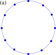
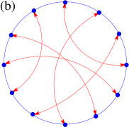
Figure 1: (a) One-dimensional (1D) regular network (with periodic boundary conditions), where nodes are connected to their nearest neighbors. (b) Small-world (SW) synchronization network, where each node is connected to exactly one randomly chosen node, in addition to the nearest neighbors.

One of the important aspects of conservative PDES is the theoretical efficiency or utilization which is defined as the average fraction of non-idling PEs at each parallel step. This measure also provides the average progress rate of the simulation, as can be seen from Eq. (1). In the BCS scheme, where only nearest-neighbor interactions are present, the utilization is equal to the density of local minima in the simulated time horizon. Thus, the utilization (on a regular one-dimensional lattice) can be written as

$$\langle u\rangle=\langle\Theta(\tau_{i-1}-\tau_{i})\Theta(\tau_{i+1}-\tau_{i})\rangle=\langle\Theta(-\phi_{i-1})\Theta(\phi_{i})\rangle\;,$$ (2)

where $\phi_{i}\equiv\tau_{i+1}-\tau_{i}$ is the local slope, $\Theta(...)$ is the Heaviside step function, and $\left\langle...\right\rangle$ denotes an ensemble average over the noise in Eq. (1). The utilization is independent of $i$ for a system of identical PEs due to the translational invariance.

Figure 2: Possible simulated-time configurations for three successive nodes (involving two successive slopes) in the basic conservative scheme (BCS) in one dimension. From the perspective of node $i$, only configuration (b) allows it to proceed (node $i$ is a local minimum). In all other cases causality could be violated if an update occurs at site $i$, because the local field variables of the neighboring nodes are not known at the instant of update attempt.

Another important observable of PDES is the statistical spread or width of the simulated time surface. The width of the simulated time surface $w$ is defined as the root mean square of the virtual times with respect to the mean, $w=\sqrt{\langle w^{2}\rangle}$, where

$$\left\langle w^{2}\right\rangle\equiv\left\langle w^{2}(N,t)\right\rangle=\left\langle\frac{1}{N^{d}}\sum_{i=1}^{N^{d}}\left[\tau_{i}(t)-\bar{\tau}(t)\right]^{2}\right\rangle\;\;,$$ (3)

and $\bar{\tau}(t)$$=$$(1/N^{d})\sum_{i=1}^{N^{d}}\tau_{i}(t)$ is the mean progress (“mean height”) of the time surface.

Since we use the formalism and terminology of non-equilibrium surface growth phenomena, we briefly review scaling concepts for self-affine or rough surfaces. The scaling behavior of the width, $\langle w^{2}(N,t)\rangle$, alone typically captures and identifies the universality class of the non-equilibrium growth process BARA95 ; HEALY95 ; KRUG97 . In a finite system the width initially grows as $\left\langle w^{2}(N,t)\right\rangle$$\sim$$t^{2\beta}$, and after a system-size dependent cross-over time $t_{\times}$$\sim$${N}^{z}$, it reaches a steady-state $\left\langle w^{2}(N,t)\right\rangle$$\sim$${N}^{2\alpha}$ for $t$$\gg$$t_{x}$. In the relations above $\alpha$, $\beta$, and $z$=$\frac{\alpha}{\beta}$ are called the roughness, the growth, and the dynamic exponent, respectively. The temporal and system-size scaling of the width can be captured by the Family-Vicsek FAMILY85 relation,

$$\left\langle w^{2}(N,t)\right\rangle=N^{2\alpha}f(t/N^{z})\;.$$ (4)

Note that the scaling function $f(x)$ depends on $t$ and the linear system-size $N$ only through the specific combination $x=t/N^{z}$, reflecting the importance of the crossover time $t_{\times}$. For small values of its argument $f(x)$ behaves as a power law, while for large arguments it approaches a constant,

$$f(x)\sim\left\{\begin{array}[]{ll}x^{2\beta}&\mbox{if $x$$\ll$$1$}\\ \mbox{const.}&\mbox{if $x$$\gg$$1$}\end{array}\right.\;,$$ (5)

yielding the correct scaling behavior of the width for early times ($x$$\ll$$1$) and for the steady-state ($x$$\gg$$1$).

A somewhat less frequently studied quantity is the growth rate of a growing surface. This quantity is typically non-universal KORN00_PRL ; TORO00 ; KRUG90 ; KORN_ACM ; KOLA03_PRE_1 ; KOLA03_PRE_2 ; KOLA04 , but as was shown by Krug and Meakin KRUG90 , on $d$-dimensional regular lattices, the finite-size corrections to it are. In the context of the basic PDES scheme, the growth rate of the simulated time surface corresponds to the progress rate (or utilization) of the simulation, hence our special interest in this observable. For the finite-size behavior of the steady-state growth rate, one has KRUG90

$$\langle u(N)\rangle\simeq\langle u(\infty)\rangle+\frac{const.}{N^{2(1-\alpha)}}\;,$$ (6)

where $\langle u(\infty)\rangle$ is the value of the growth rate in the asymptotic infinite system-size limit and $\alpha$ is the dimension-dependent roughness exponent of the growth process.

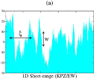
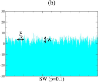
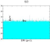
Figure 3: Virtual time horizon snapshots for 10,000 sites in 1D. (a) For the regular network with nearest-neighbor connections ($p$=$0$). The lateral correlation length $\xi$ and width $w\equiv\sqrt{w^{2}}$ are shown for illustration in the graph. The rough steady-state surface belongs to the KPZ/EW universality class. For the SW synchronization network with (b) $p$$=$$0.1$ and (c) $p$$=$$1$ the heights are effectively decorrelated and both the correlation length and the width are reduced, and approach system-size independent values for sufficiently large systems. The resulting surface is macroscopically smooth. Note that the heights are relative to the average height.

Based on a mapping between virtual times and surface heights KORN00_PRL , in the coarse-grained description, the virtual time horizon of the BCS was found to be governed KORN00_PRL ; TORO00 by the Kardar-Parisi-Zhang (KPZ) equation KARD86 , well-known in surface growth phenomena

$$\partial_{t}\hat{\tau}_{i}=\nabla^{2}\hat{\tau}_{i}-\lambda(\nabla\hat{\tau}_{i})^{2}+...+\eta_{i}(t)\;,$$ (7)

where $\nabla^{2}$ stands for the discretized Laplacian, $\nabla^{2}\hat{\tau}_{i}=\hat{\tau}_{i+1}+\hat{\tau}_{i-1}-2\hat{\tau}_{i}$, $\nabla$ is the discretized gradient operator, $\nabla\hat{\tau}_{i}=\hat{\tau}_{i+1}-\hat{\tau}_{i}$, $\hat{\tau}_{i}=\tau_{i}-\bar{\tau}$ is the surface height fluctuation (or virtual time) measured from the mean, $\eta_{i}(t)$ is a noise delta-correlated in space and time, $\langle\eta_{i}(t)\eta_{j}(t^{\prime})\rangle=2D\delta_{ij}\delta(t-t^{\prime})$, $\lambda$ is a positive constant and $...$ stands for higher order irrelevant terms (in a renormalization group sense). Equation (7) can also give an account of a number of other nonlinear phenomena such as Burgers turbulence and directed polymers in random media BARA95 . When the simple update rule of the basic synchronization scheme is implemented on a one-dimensional regular network, one can observe a simulated time surface governed by the KPZ equation, and in the steady-state, by the Edwards-Wilkinson Hamiltonian EDWARDS82 [Fig. 3(a)].

When analyzing the statistical and morphological properties of the stochastic landscape of the simulated times, it is convenient to study the height-height correlation or its Fourier transform, the height-height structure factor. The equal-time height-height structure factor $S(k,t)$ in one-dimension is defined as

$$S(k,t)N\delta_{k,-k^{\prime}}=\langle\tilde{\tau}_{k}(t)\tilde{\tau}_{k^{\prime}}(t)\rangle\;,$$ (8)

where $\tilde{\tau}_{k}=\sum_{j=1}^{N}e^{-ikj}\tau_{j}$ is the Fourier transform of the virtual times with the wave number $k$=$2\pi n/N$, $n$=$0,1,2,...,N-1$ and $\delta_{k,-k^{\prime}}$ is the Kronecker delta. The structure factor essentially contains all the “physics” needed to describe the scaling behavior of the time surface. Here we focus on the steady-state properties ($t$$\to$$\infty$) of the time horizon where the structure factor becomes independent of time, $\lim_{t\to\infty}S(k,t)=S(k)$. In the long-time limit in one dimension, for a KPZ surface described by Eq. (7) one has TORO00

$$S(k)=\frac{D}{2[1-\cos(k)]}\sim\frac{1}{k^{2}}\;,$$ (9)

where the latter approximation holds for small values of $k$. By performing the inverse Fourier transformation of Eq. (9), we can also obtain the spatial two-point function,

$$G(l)=(1/N)\sum_{k\neq 0}e^{ikl}S(k)\;,$$ (10)

yielding TORO00 ; TORO03

$$G(l)\simeq\frac{D}{2}\left(\frac{N}{6}-l\right)$$ (11)

for $1\ll l\ll N$. In particular, for the steady-state width one finds

$$\langle w^{2}\rangle=\frac{1}{N}\sum_{k\not=0}S(k)=G(0)\simeq\frac{D}{12}N\sim N$$ (12)

in one dimension TORO00 . This divergent width is caused by a divergent length scale, $\xi$, the “lateral” correlation length in the KPZ-like synchronization landscape.

The measured steady-state structure factor [Fig. 4(a)], obtained by simulating the BCS based on the exact rules for the evolution of the synchronization landscape, confirms the coarse-grained prediction for small $k$ values, $S(k)\sim 1/k^{2}$. Figure 4(b) shows the corresponding spatial two-point correlation function $G(l)$.

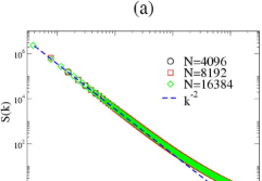
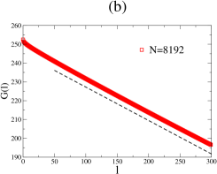
Figure 4: (a) The steady-state structure factor as a function of the wave number for the BCS scheme in 1D. The small-$k$ course-grained prediction (consistent with the steady-state EW/KPZ universality class in 1D) is indicated by a dashed line [Eq. (9)]. Note the log-log scales. (b) Steady-state spatial two-point correlation function. The straight line again indicates the asymptotic EW/KPZ behavior in one dimension [Eq. (11)].

Simulations of the BCS scheme in one dimension yield scaling exponents that agree within error with the predictions of the KPZ equation BARA95 ; HEALY95 ; KARD86 . The time evolution of the width [Fig. 5(a)] shows that the growth exponent $\beta$$\simeq$$1/3$. Looking at the system-size dependence of the steady-state width [Figure 5(b)], we find the roughness exponent $\alpha$$\simeq$$1/2$, consistent with the one-dimensional KPZ value, $\langle w^{2}\rangle$$\sim$$N^{2\alpha}$$\sim$$N$. The dynamic exponent values found from the width as a function of the cross-over time and $z$=$\alpha/\beta$ are the same, about $3/2$. The inset in Fig. 5(a) shows that the scaled version of the width evolution by using the scaling exponents is consistent with the Family-Vicsek relation [Eq. (4)], although with relatively large corrections to scaling.

The width distributions, $P(w^{2})$, have been introduced to provide a more detailed characterization of surface growth processes FOLTIN94 ; PLISCHKE94 ; RACZ94 ; ANTAL96 ; ANTAL2001 ; ANTAL2002 and have been used to identify universality classes KORN00_PRL . The width distribution of rough surfaces belonging to the same universality class is governed by a universal scaling function $\Phi(x)$, such that $P(w^{2})$$=$$\langle w^{2}\rangle^{-1}\Phi(w^{2}/\langle w^{2}\rangle)$. $\Phi(x)$ can be calculated analytically for a number of models, including the EW class FOLTIN94 . The width distribution for the basic synchronization scheme is shown in Fig. 5(c). Systems with $N$$\geq$$10^{3}$ show convincing data collapse onto this exact scaling function. The inset in Fig. 5(c) shows the same graph in log-normal scale to show the collapse at the tail of the distribution. The convergence to the limit distribution is very slow when compared to other microscopic models (such as the single-step model BARA95 ; ANTAL96 ) belonging to the same universality class.

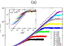
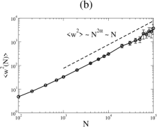
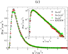
Figure 5: (a) Time evolution of the width for different system-sizes in the BCS scheme in 1D. The inset shows the same data on scaled axes, $\langle w^{2}\rangle/N^{2\alpha}$ versus $t/N^{z}$. Each curve has been obtained by averaging over at least fifty realizations. (b) The steady-state width of the time horizon for the one-dimensional BCS as a function of system-size. The dashed straight line represents the asymptotic one-dimensional KPZ/EW behavior, $\left\langle w^{2}(N)\right\rangle$$\sim$$N^{2\alpha}$ with $\alpha$$=$$1/2$. (c) Scaled width distributions for the BCS scheme in 1D. The exact asymptotic EW/KPZ width distribution FOLTIN94 is shown with a dashed line. The inset shows the same distributions on log-normal scales.

Now we discuss our findings for the steady-state utilization of the BCS scheme. As stated above, the synchronization landscape of the virtual times belongs to the EW universality class in one dimension. This implies that the local slopes in the steady-state landscape are short-range correlated TORO00 . Hence the density of local minima in the synchronization landscape, and in turn the utilization, remains nonzero in the infinite system-size limit KORN00_PRL ; TORO00 . For fixed $N$, the utilization drops from relatively higher initial value at early times to its steady-state value in a very short time [Fig. 6]. Further, the steady-state utilizations for various systems converge to the asymptotic system-size independent value.

Figure 6: Utilization in the 1D BCS scheme as a function of time for various system sizes. The inset shows the steady-state utilization as a function of the $1/N^{2(1-\alpha)}$ with the 1D KPZ roughness exponent $\alpha$$=$$1/2$. The dashed line is a linear fit to Eq. (6) with $\alpha$$=$$1/2$, $\langle u(N)\rangle\approx 0.2464+0.2219/N$.

In 1D, where $\alpha$$=$$1/2$, the system-size dependence of the steady-state utilization must follow [Eq. (6)] $\langle u(N)\rangle\simeq\langle u(\infty)\rangle+\frac{const.}{N}$, as confirmed by our direct simulations for the BCS scheme [inset of Fig. 6]. For the KPZ model [Eq. (7)] $\langle u(\infty)\rangle$$=$$1/4$, since in the steady state, the local slopes are delta-correlated, resulting in a probability of $1/4$ for the configuration in Fig. 2(b), corresponding to a local minimum. For the actual BCS synchronization profile $\langle u(\infty)\rangle$$\simeq$$0.2464$ KORN00_PRL ; TORO00 , as a result of non-universal short-range correlations present for the slopes in the specific microscopic model TORO03 . Finally one can argue that the utilization for the BCS on regular lattices remains nonzero in the thermodynamic limit and it displays universal finite-size effects KORN_ACM ; KOLA03_PRE_1 ; KOLA03_PRE_2 ; KOLA04 ; KRUG90 . Note that a small change with respect to the “worst case” (one-site-per PE) scenario, in particular, hosting more than one site per PE, leads to utilizations that are close to the limiting value of unity KOLA03_PRE_1 ; KOLA04 , and hence are practical for actual PDES implementations KORN99_JCP ; AMAR_PRB_2005a ; AMAR_PRB_2005b .

In order to obtain an analytically tractable scalability model for the BCS scheme, Greenberg et al. introduced the $K$-random interaction network model GREEN96 . In this model at each update attempt PEs compare their local simulated times with those of a set of $K$ randomly chosen PEs. This set is re-chosen for each update attempt (i.e., the network is “annealed”), even if a previous update attempt has failed. It was shown that in the limit of $t$$\to$$\infty$ and $N$$\to$$\infty$, the utilization (or the average rate of progress) converges to a non-zero constant, $1/(K+1)$. They also suggested that the scaling properties of $K$-random model as $t$$\to$$\infty$ and $N$$\to$$\infty$ are universal and hold for regular lattices as well. But changing the interaction from nearest neighbor PEs on a regular lattice to randomly chosen PEs changes the universality class of the time horizon. Simply put, the underlying topology has crucial effects on the universal behavior of the time horizon. The random (annealed) interaction topology of the $K$-random model results in a mean-field-like behavior, where the simulated time surface is uncorrelated and has a finite width in the limit of an infinite number of PEs. Their conjecture for the width does not hold, thus, the BCS scheme for regular lattices cannot be equivalently described by the $K$-random model (at least not below the upper critical dimension of the KPZ universality class MARINARI02 ). However, we were inspired by GREEN96 to change the communication topology of the PEs by introducing random links in addition to the necessary short-range connections. In the next section we present our modification to the original conservative scheme on regular lattices to achieve a fully scalable algorithm where both scalability conditions are satisfied: the simulation has a nonzero progress rate and the width of the synchronization landscape is finite.

III Small-World Synchronization Scheme in 1D

The divergent width for the larger systems, discussed in the previous section, is the result of the divergent lateral correlation length $\xi$ of the virtual time surface, reaching the system-size $N$ in the steady-state BARA95 ; KORN_ACM ; KOLA03_PRE_1 ; KOLA03_PRE_2 ; KOLA04 . To de-correlate the simulated time horizon, first, we modify the virtual communication topology of the PEs. The resulting communication network must include the original short-range (nearest-neighbor) connections to faithfully simulate the dynamics of the underlying system. In the modified network, the connectivity of the nodes (the number of neighbors) should remain non-extensive (i.e., only a finite number of virtual neighbors per node is allowed). This is in accordance with our desire to design a PDES scheme where no global intervention or synchronization is employed (PEs can only have $O(1)$ communication exchanges per step). It is clear that the added synchronization links (or at least some of them) have to be long range. Short range links alone would not change the universality class and the scaling properties of the width of the time horizon. One can satisfy this condition by selecting the additional links called “small-world” links randomly among all the nodes in the network. Also, fluctuations in the individual connectivity should be avoided for load balancing purposes, i.e., requiring the same number of added links (e.g., one) for each node is a reasonable constraint. We then choose the extra synchronization links in such a way that each PE is connected to exactly one other PE via a “quenched” bidirectional link [Fig. 1(b)].

One of the basic structural characteristics of SW-like networks is the “low degree of separation” between the nodes. The most commonly used observables to analyze this property are the average shortest path length, $\delta_{avg}(N)$, and the maximum shortest path length, $\delta_{max}(N)$. The shortest path length between two nodes is defined as the minimum number of nodes needed to visit in order to go from one of the nodes to the other. The average shortest path length is obtained by averaging the above quantity between all possible pairs of nodes in a given network. The maximum shortest path length, also known as the diameter of the network, is the length of the longest among the shortest paths in the network. Both of these observables scale logarithmically with the system-size $N$ in SW-like networks BOLLOBAS . The system-size dependence of these path lengths for our one-dimensional SW network is logarithmic as expected, see Fig. 7.

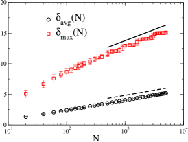
Figure 7: Average and maximum shortest path (diameter) as a function of the number of nodes for the SW synchronization network in 1D, as described in the text. The latter is also referred to as the diameter of the network. The solid and dashed lines both indicate the logarithmic dependence. Note the normal-log scales.

We now describe the modified algorithmic steps for the SW connected PEs KORN03_SCI . In the SW conservative PDES scheme, in every parallel time step, each PE, with probability $p$, compares its local simulated time with its full virtual neighborhood, and can only advance if it is the minimum in this neighborhood, i.e., if $\tau_{i}(t)$$\leq$$\min\{\tau_{i-1}(t),\tau_{i+1}(t),\tau_{r(i)}(t)\}$, where $r(i)$ is the random connection of PE $i$. With probability $(1$$-$$p)$ each PE follows the original scheme, i.e., the PE then can advance if $\tau_{i}(t)$$\leq$$\min\{\tau_{i-1}(t),\tau_{i+1}(t)\}$. Our network model including the nearest neighbors and random SW links can be seen in Fig. 1(b). Note that the occasional extra checking of the simulated time of the random neighbor is not needed for the faithfulness of the simulation KORN03_SCI . It is merely introduced to control the width of the time horizon. The occasional checking of the virtual time of the random neighbor (with rate $p$) introduces an effective strength $J$$=$$J(p)$ for these links. Note that this is a dynamic “averaging” process controlled by the parameter $p$ and can possibly be affected by nonlinearities in the dynamics through renormalization effects. The exact form of $J(p)$ is not known. The only plausible assumption we make for $J$ is that it is a monotonically increasing function of $p$ and is only zero when $p$=$0$.

In what follows, we focus on the characteristics of the synchronization dynamics on the network. As we have seen for the one-dimensional regular network, the communication topology between the nodes (up to linear terms) leads to simple relaxation, governed by the Laplacian on the regular grid. Random communication links give rise to analogous effective couplings between the nodes, corresponding to the Laplacian on the random part of the network. Thus, the large-scale properties of the virtual time horizon of our SW scheme are governed by the effective Langevin equation

$$\partial_{t}\hat{\tau}_{i}=\nabla^{2}\hat{\tau}_{i}-\sum_{j}J_{ij}(\hat{\tau}_{i}-\hat{\tau}_{j})+...+\eta_{i}(t)\;,$$ (13)

where the … stands for infinitely many non-linear terms (involving non-linear interactions through the random links as well), and $J_{ij}$ is proportional to the symmetric adjacency matrix of the random part of the network: $J_{ij}$$=$$J(p)$ if sites $i$ and $j$ are connected by a random link and $J_{ij}$$=$$0$ otherwise. For our specific SW construction each node has exactly one random neighbor, i.e. there are no fluctuations in the individual connectivity (degree) of the nodes. Our simulations (to be discussed below) indicate that when considering the large-scale properties of the systems, the Laplacian on the random part of the network generates an effective coupling $\gamma$ to the mean value of the fluctuations in the synchronization landscape $\overline{\tau}$ KORN03_SCI . At the level of the structure factor, it corresponds to an effective mass $\gamma$ (in a field-theory sense)

$$S(k)\propto\frac{1}{\gamma+k^{2}}\;,$$ (14)

where $\gamma$$=$$\gamma(p)$ is a monotonically increasing function of $p$ with $\gamma(0)$=$0$.

We emphasize that the above is not a derivation of Eq. (14), but rather a “phenomenological” description of our findings. It is also strongly supported by exact asymptotic results for the (linear) EW model on SW networks, where the effect of the Laplacian on the random part of the network is to generate an effective mass KOZMA03 ; KOZMA05b . The averaging over the quenched network ensemble, however, can introduce nontrivial scaling and corrections in the effective coupling KOZMA03 ; KOZMA05b ; KOZMA05 . In our case, this is further complicated by the nonlinear nature of the interaction. The results of “simulating the simulation”, however, suggest that the dynamic control of the link strength and nonlinearities only give rise to a renormalized coupling and a corresponding renormalized mass. Thus, the dynamics of the BCS scheme with random couplings is effectively governed by the EW relaxation in a small-world KOZMA03 ; KOZMA05b ; KOZMA05 .

From Eq. (14) it directly follows that the lateral correlation length, in the infinite system-size limit, scales as

$$\xi\sim\gamma^{-1/2}\;,$$ (15)

i.e., becomes finite for all $p\not$=$0$. The presence of the effective mass term in the structure factor in Eq. (14) implies that $\lim_{k\rightarrow 0}S(k)$$<$$\infty$, that is, there are no large amplitude long-wavelength modes in the surface. Consequently, the width $\langle w^{2}\rangle$$=$$(1/N)\sum_{k\not=0}S(k)\sim\xi$ is also finite. Our simulated time landscapes indeed show that they become macroscopically smooth when SW links are employed [Figs. 3(b) and 3(c)], compared to the the same dynamics with only short-range links [Fig. 3(a)].

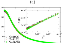
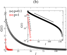
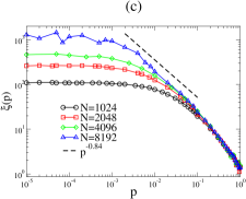
Figure 8: (a) Structure factor for the 1D SW synchronization scheme with $p$=$0.1$. The inset shows $1/S(k)$ vs. $k^{2}$ for small values of $k$, confirming the coarse-grained prediction Eq. (14). (b) The spatial two-point correlation function as a function of (the Euclidean) distance $l$ between the nodes for two different values of $p$, indicating an exponential decay with an average correlation length $\xi$$\approx$$27$ and $\xi$$\approx$$1.6$ for $p$=$0.1$ and $p$=$1$, respectively. The inset shows the same data on log-normal scales. (c) Correlation length vs. $p$ for different system-sizes. The dashed line corresponds to the estimate of the exponent $s$, $\xi(p)\sim p^{-s}$ with $s$$\approx$$0.84$, in the small-$p$ regime for an asymptotically infinite system.

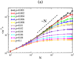
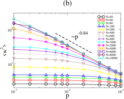
Figure 9: (a) The average steady-state width in the 1D SW synchronization landscape as a function of the system size for different values of $p$ in the range of $[10^{-3},10^{-1}]$. The dashed line indicates the EW/KPZ scaling, corresponding to the small system-size behavior. (b) The average steady-state width in the 1D SW synchronization landscape as a function of $p$ for different values of $N$ in the range of $[40,10^{4}]$. The dashed line indicates the best-fit power law in the asymptotic large-$N$ small-$p$ regime to extract the correlation length exponent $s$, according to Eqs. (16)-(18).

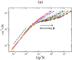
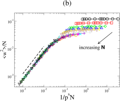
Figure 10: The scaled versions of Figs. 9(a) and (b), as proposed by Eqs. (16)-(18) by plotting $\left\langle w^{2}\right\rangle/N$ vs. $1/p^{s}N$ with $s$=$0.84$. The data points are identical in (a) and (b), but data points connected by a line have the same value of $p$ in (a) and have the same value of $N$ in (b), as obtained by rescaling Figs. 9(b) and (b), respectively. The dashed line corresponds to the asymptotic small-$x$ behavior of the scaling function $g(x)$ [Eq. (17)].

In the simulations, we typically performed averages over 10-100 network realizations, and compared the results to those of individual runs. Our results indicate that the observables we studied (the width and its distribution, the structure factor, and the utilization) display strong self-averaging properties, i.e., for large enough systems, they become independent of the particular realization of the underlying SW network. Simulation results for the structure factor, $S(k)$, for the SW synchronization scheme are shown in Fig. 8(a). If an infinitesimally small $p$ is chosen, $S(k)$ approaches a finite constant in the limit of $k$$\rightarrow$$0$, and in turn, the virtual time horizon becomes macroscopically smooth with a finite width.

A possible (phenomenological) way to obtain the correlation length is to fit our structure factor data to Eq. (14), more specifically, by plotting $1/S(k)$ versus $k^{2}$, which exhibits a linear relationship. By a linear fit, $\gamma$ is then the ratio of the intercept and the slope (inset in Fig. 8(a)). Alternatively, one can confirm that the massive propagator in Eq. (14) indeed leads to an exponential decay in the two-point correlation function $G(l)$ from which the correlation length can also be extracted [Fig. 8(b)]. In our case with a system-size $N$=$16384$ it is $\xi$$\approx$$27$ for $p$=$0.1$ and $\xi$$\approx$$1.6$ for $p$=$1$. Fig. 8(c) shows the correlation length extracted from the structure factor $S(k)$ as a function of $p$ for different system-sizes.

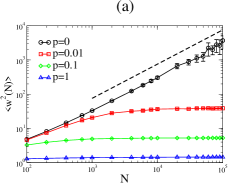
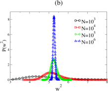
Figure 11: (a) The average steady-state width as a function of system-size for different values of $p$ in the 1D SW synchronization scheme. The $p$$=$$0$ case corresponds to the purely 1D BCS scheme (exhibiting EW/KPZ scaling, indicated by a dashed line) and is also shown for comparison. Steady-state width distributions in the 1D SW synchronization scheme for (b) $p$=$0.1$ and for (c) $p$=$1$. The distributions were constructed using ten different network realizations, except for $N$=$10^{6}$, where only one realization was obtained due to computational limitations. All width distributions, however, indicated self-averaging.

An alternative way to determine the correlation length is to attempt a finite-size scaling analysis of the width $\langle w^{2}\rangle$. There are two length scales in the system: the linear system size $N$ and the correlation $\xi$ of an infinite system. For $p$$=$$0$, $\langle w^{2}\rangle$$\sim$$N$, while for $p$$>$$0$ and $N$$\to$$\infty$, $\langle w^{2}\rangle$$\sim$$\xi$. For non-zero $p$ and finite $N$ the scaling of the width can be expected KOZMA05 ; KORN_PLA_swrn to follow

$$\left\langle w^{2}\right\rangle=Ng(\xi/N)\;,$$ (16)

where $g(x)$ is a scaling function such that

$$g(x)\sim\left\{\begin{array}[]{ll}x&\mbox{if $x$$\ll$$1$}\\ \mbox{const.}&\mbox{if $x$$\gg$$1$}\end{array}\right.\;.$$ (17)

For non-zero $p$ and for sufficiently small systems ($N$$\ll$$\xi(p)$) one can confirm that the behavior of the width follows that of the system without random links $\langle w^{2}\rangle\sim N$ [Fig. 9(a)]. For large-enough systems, on the other hand, we can extract the $p$-dependence of the infinite-system correlation length as $\langle w^{2}\rangle\sim\xi(p)$ [Fig. 9(b)], yielding

$$\xi(p)\sim p^{-s}\;,$$ (18)

where $s\approx 0.84$.

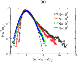
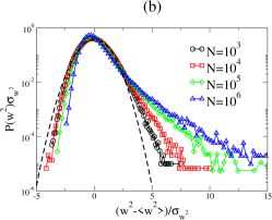
Figure 12: Steady-state width distributions for the 1D SW synchronization scheme scaled to zero mean and unit variance for (a) $p$=$0.1$ and (b) $p$=$1$. The dashed curves are similarly scaled Gaussians for comparison.

We then studied the data collapse as proposed by Eq. (16) by plotting $\langle w^{2}\rangle/N$ vs. $1/p^{s}N$. In fact, we performed this rescaling originating from both raw data sets Figs. 9(a) and (b). The resulting scaled data points in Fig. 10(a) and (b), of course, are identical in the two figures, but the lines connect data points with the same value of $p$ in Fig. 10(a) and with the same value of $N$ in Fig. 10(b). These scaled plots in Fig. 10 indicate that there are very strong corrections to scaling: data for larger $p$ or smaller $N$ values peel off from the proposed scaling form Eq. (17) relatively quickly. These strong corrections are possibly the result of the nonlinear nature of the interaction between the nodes on the quenched network. We note that the purely linear EW model on identical networks exhibits the scaling proposed in Eqs. (16) and (17) without noticeable corrections to scaling KOZMA05 ; KORN_PLA_swrn .

The non-zero $\gamma$, leading to a finite correlation length, $\xi$, ensures a finite width in the infinite system-size limit. Our simulations show that the width saturates to a finite value for $p$$>$$0$ [Fig. 11(a)]. The distribution of the steady-state width $P(w^{2})$ changes from that of the EW/KPZ class to a delta function for non-zero values of $p$ as the system size goes to infinity. Figure 11(b) and (c) shows the width distributions for $p$=$0.1$ and $p$=$1$, respectively. The scaled width distributions (to zero mean and unit variance), however, exhibit the convergence to a delta function through nontrivial shapes for different values of $p$. For $p$=$0.1$ [Fig. 12(a)] the distributions appear to slowly converge to a Gaussian as the system-size increases. For $p$=$1$ [Fig. 12(b)], the trend is opposite, up to the system sizes we could simulate; as the system-size increases, the distributions exhibit progressively non-Gaussian features (closer to an exponential) around the center, for up to $N$=$10^{6}$. Note that not only the average width $\langle w^{2}\rangle$, but also the full distribution $P(w^{2})$ was found to be self-averaging, i.e., independent of the particular realization of the underlying SW network, so the above effect is not due to insufficient averaging over network realizations. Since we were intrigued by the above change in the trend of the convergence (i.e., away from vs. toward the Gaussian), we carried out some exploratory simulations for a range of $p$ values and evaluated the kurtosis and the skewness of the width distributions. The results shows that this change occurs at around $p\approx 0.9$. We could not conclude, however, whether this change corresponds to an actual transition and the emergence of a strong disordered-coupling regime, where the distribution of the width is a delta function, centered about a finite value, but, the limiting shape of the delta function is non-Gaussian, or to the development of strong non-monotonic finite-size effects.

Figure 13: Steady-state utilization of SW synchronization network in 1D as a function of system-size for three different values of $p$$=$$0$ (BCS), $p$$=$$0.1$ and $p$$=$$1$.

The effect of the random communication links on the utilization can be understood as follows. According to the algorithmic rules, the virtual times of the full network neighborhood (including the random neighbor) are checked with probability $p$, while with probability $(1$$-$$p)$ only short-ranged synchronization is employed. Thus, the average progress rate of the simulated times becomes

$$\langle u\rangle = (1-p)\langle\Theta(-\phi_{i-1})\Theta(\phi_{i})\rangle+p\langle\Theta(-\phi_{i-1})\Theta(\phi_{i})\Theta(\tau_{r(i)}-\tau_{i})\rangle$$ (19)

$$= \langle\Theta(-\phi_{i-1})\Theta(\phi_{i})\rangle-p\left[\langle\Theta(-\phi_{i-1})\Theta(\phi_{i})\rangle-\langle\Theta(-\phi_{i-1})\Theta(\phi_{i})\Theta(\tau_{r(i)}-\tau_{i})\rangle\right]\;.$$

Note that performing disorder averaging (over random network realizations) makes the right hand side independent of $i$. In the presence of the SW links the regular density of local minima $\langle\Theta(-\phi_{i-1})\Theta(\phi_{i})\rangle$ remains nonzero (in fact, increases, compared to the short-range synchronized BCS scheme) GUCLU_CNLS ; TORO03 ; KORN03_SCI . Thus, for an infinitesimally small $p$, the utilization, at most, can be reduced by an infinitesimal amount, and the SW-synchronized simulation scheme maintains a nonzero average progress rate. This can be favorable in PDES where scalable global performance requires both finite width and nonzero utilization. With the SW synchronization scheme, both of these objectives can be achieved. For example, for $p$$=$$0.1$ $\langle u\rangle_{\infty}\simeq 0.242$, while for $p$$=$$1$ $\langle u\rangle_{\infty}\simeq 0.141$. The steady-state utilization as a function of system size for various values of $p$ can be seen in Fig. 13.

IV Basic Conservative Synchronization Scheme in 2D

A natural generalization to pursue is the same synchronization dynamics and the associated landscapes on networks embedded in higher dimensions. One might ask whether PDES of two-dimensional phenomena exhibit kinetic roughening of the virtual time horizon. Preliminary results indicated that this is the case KORN00_UGA ; KIRKPATRICK03 . In this section we give detailed results when the BCS scheme is extended onto a two-dimensional lattice ($N_{PE}$$=$$N^{2}$, $N$ being the linear size) in which each node has four nearest neighbors. We consider a system with periodic boundary conditions in both axis as can be seen in Fig. 14(a). The same microscopic rules, i.e. each node increments its local simulated time by an exponentially distributed random amount when it is a local minima among its nearest neighbors, are applied to this lattice. As in the one-dimensional case, during the evolution of the local simulated times correlations between the nodes develop in the system. One observes rough time surfaces in the steady-state after simulating this system. Figure 15(a) shows the contour plot of the simulated time surface for the BCS scheme in 2D.

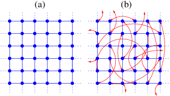
Figure 14: Communication topologies in 2D. (a) 2D regular network, where each node is connected to its four nearest neighbors. (b) SW synchronization network. One random link per node is added on top of the 2D regular network. Red arrows show the bidirectional random links between the nodes.

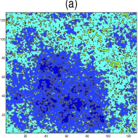
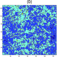
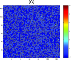
Figure 15: Synchronization landscapes as contour plots for the 2D BCS on regular and SW networks of 128x128 nodes. (a) for the BCS scheme on a regular lattice with only nearest-neighbor connections (equivalent to $p$=$0$); (b) for $p$=$0.1$; (c) for $p$=$1$.

In 2D as well, we observe kinetic roughening of the BCS scheme. The simulated time surface for a finite system initially roughens with time in a power-law fashion. It then saturates after some system-size dependent crossover time to its system-size dependent steady-state value, as shown in [Fig. 16(a)]. Our estimate for the growth exponent in the early-time regime is $\beta$$=$$0.125$, significantly smaller than in one dimension.

The roughness exponent $\alpha$ for KPZ-like systems have been measured and estimated in a number of experiments and simulations BARA95 . Since exact exponents for the higher-dimensional KPZ universality class are not available, for reference, we compare our results to a recent high-precision simulation study by Marinari et al. MARINARI00 on the restricted solid-on-solid (RSOS) model KIM89 , a model believed to belong to the KPZ class. They found in Ref. MARINARI00 that $\alpha$$\simeq$$0.39$ for the 2D RSOS roughness exponent. While our simulations of the virtual time horizon show kinetic roughening in Fig. 16(a), the scaled plot, suggested by Eq. (4), indicates very strong corrections to scaling for the BCS in 2D [Fig. 16(a) inset]. Figure  16(b) and (c) also indicates that the (KPZ) scaling regime is approached very slowly, which is not completely unexpected: for the 1D BCS scheme as well, convergence to the steady-state roughness exponent Fig. 5(a) and to the KPZ width distribution Fig. 5(b) only appears for linear system sizes $N$$>$${\cal O}(10^{3})$. Here, for the 2D case, the asymptotic roughness scaling [Fig. 16(b)] and width distribution [Fig. 16(c)] has not been reached for the system sizes we could simulate (up to linear system size $N$$=$$2048$). Nevertheless the trend in the finite-size behavior, and the identical microscopic rules (simply extended to 2D) suggest that 2D BCS landscape belongs to the 2D KPZ universality class.

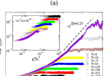
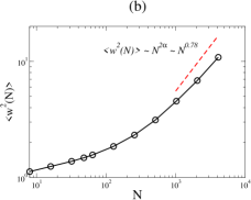
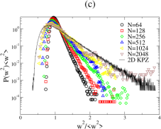
Figure 16: (a) Time evolution of the width in 2D BCS scheme. The dashed line indicates the power-law behavior of the width before saturation with a growth exponent $\beta$$\approx$$0.125$. The inset shows the scaled plot $\left\langle w^{2}\right\rangle/N^{2\alpha}$ vs. $t/N^{z}$. (b) Steady-state width of the 2D BCS scheme as a function of the linear system-size. The dashed line corresponds to the asymptotic 2D KPZ scaling with roughness exponent $2\alpha$$=$$0.78$ as obtained by high-precision simulations of the RSOS model MARINARI00 . Note the log-log scales. (c) The scaled width distributions for the 2D BCS scheme. The solid curve is the asymptotic 2D KPZ scaled width distribution, again from high-precision RSOS simulations MARINARI02 . Note the log-normal scales.

For further evidence, we also constructed the structure factor for the 2D BCS steady-state landscape. As shown in Fig. 17(a), $S(k_{x},k_{y})$ exhibits a strong singularity about ${\bf k}={\bf 0}$. For further analysis, we exploited the symmetry of $S(k_{x},k_{y})$ that it can only depend on $|{\bf k}|=\sqrt{k_{x}^{2}+k_{y}^{2}}$. Hence, we averaged over all directions having the same wave number $|{\bf k}|$ to obtain $S(|{\bf k}|)$. For small wave numbers we found that it diverges as

$$S(|{\bf k}|)\sim\frac{1}{|{\bf k}|^{2+2\alpha}}\;,$$ (20)

with $\alpha=0.39$, as shown in Fig. 17(b). This is consistent with the small-$k$ behavior of the structure factor of the 2D KPZ universality class with roughness exponent $\alpha$$\simeq$$0.39$ MARINARI00 . As noted above, the scaling of the width and its distribution exhibited very slow convergence to those of our “reference”-KPZ system, the RSOS model MARINARI00 ; MARINARI02 . This is likely the effect of the non-universal and surprisingly large contributions coming from the large-$k$ modes, leading to very strong corrections to scaling for the system sizes we were able to study in 2D. Looking directly at the small-$|{\bf k}|$ behavior of $S(|{\bf k}|)$ is, of course, undisturbed by the larger-$|{\bf k}|$ modes, hence the relatively good agreement with the 2D KPZ scaling.

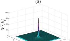
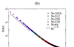
Figure 17: Structure factor for the BCS scheme in 2D. (a) as a function of the wave number components $k_{x}$ and $k_{y}$. (b) as a function of the magnitude of the wave number for different system-sizes. The dashed line shows the asymptotic 2D KPZ behavior for small values of $|{\bf k}|$ [Eq. (20)] with $\alpha$$=$$0.39$ MARINARI00 . Note the log-log scales.

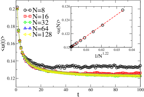
Figure 18: The time evolution of the steady-state utilization in 2D BCS scheme for various system sizes. The inset shows the steady-state utilization in the 2D BCS scheme as a function of $1/N^{2(1-\alpha)}$ with the 2D KPZ roughness exponent $\alpha$$=$$0.39$. The dashed line is a linear fit to Eq. (6) with $\alpha$$=$$0.39$, $\langle u(N)\rangle\approx 0.1201+0.1585/N^{1.22}$.

The steady-state utilization (density of local minima) in the 2D BCS synchronization landscape approaches a nonzero value in the limit of an infinite number of nodes, $\langle u(\infty)\rangle$$\simeq$$0.1201$ as can be seen in Fig. 18. This is consistent with the general approximate behavior $\langle u(\infty)\rangle\simeq const./d$ on hypercubic lattices in $d$ dimension GREEN96 ; KORN00_UGA , i.e., $\langle u(\infty)\rangle$ is approximately inversely proportional to the coordination number. As shown in Fig. 18 (inset), for a two-dimensional BCS scheme, the steady-state utilization scales as [Eq. (6)] $\langle u(N)\rangle\simeq\langle u(\infty)\rangle+\frac{const.}{N^{1.22}}$, where we have used the 2D KPZ roughness exponent $\alpha$$=$$0.39$ MARINARI00 .

V Small-World Synchronization Scheme in 2D

The de-synchronization (roughening of the virtual time horizon) again motivates the introduction of the possibly long-range, quenched random communication links on top of the 2D regular network. Each node has exactly one (bi-directional) random link as illustrated in Fig. 14(b). The actual “microscopic” rules are analogous to the 1D SW case: with probability $p$ each node will check the local simulated times of all of its neighbors, including the random one, and can increment its local simulated time by an exponentially distributed random amount, only if it is a “local” minimum (among the four nearest neighbors and its random neighbor). With probability $(1$$-$$p)$, only the four regular lattice neighbors are checked for the local minimum condition.

The effect of the synchronization through the random links is, again, to stop kinetic roughening and to suppress fluctuations in the synchronization landscapes. Contour plots of the synchronization landscapes are shown in Figure 15(b) and (c) for $p$$=$$0.1$ and $p$$=$$1$, respectively. Our results indicate that for any nonzero $p$ the width of the surface approaches a finite value in the limit of $N$$\to$$\infty$ [Fig. 19(a)]. At the same time, the width distribution approaches a delta-function in the large system-size limit as shown in Figs. 19(b) and 19(c). The scaled distributions (to zero mean and unit variance) again show that at least for the finite systems we observed, the shape of these distribution differs from a Gaussian. The deviation from the Gaussian around the center of the distribution is stronger for a larger value of $p$ where the influence of the quenched random links are stronger. Note that for the 1D SW landscapes as well, the width distribution only displayed a crossover to Gaussian behavior for smaller values of $p$ and for very large linear system sizes ($N$$>$${\cal O}(10^{4})$. In the 2D SW case, these linear system sizes are computationally not attainable, and the convergence to a Gaussian width distribution, or the existence of an inherently different strong-disorder regime (as a result of strong random links), remains an open question.

The underlying reason for the finite width is again a finite average correlation length between the nodes. The 2D structure factor exhibits a massive behavior, i.e., $S(|{\bf k}|)$ approaches a finite value in the limit of ${\bf k}$$\to$${\bf 0}$ [Figs. 21(a) and 21(b)]. For small wave numbers, the approximate behavior of the structure factor is again $S(|{\bf k}|)$$\propto$$1/(|{\bf k}|^{2}+\gamma)$ as can be seen in the inset of Fig. 21(b), with strong finite-size corrections to $\gamma$. The relevant feature of the synchronization dynamics on a SW network is the generation of the effective mass $\gamma$. Nonlinearities can give rise to a renormalized mass, but the relevant operator is the Laplacian on the random network.

In the 2D SW synchronization scheme the steady-state utilization is smaller than its purely 2D counterpart (BCS in 2D), as a result of the possible additional checking with the random neighbors. For small values of $p$, however, it is reduced only by a small amount, and remains nonzero in the limit of an infinite number of nodes [Fig. 22]. For example, for $p$$=$$0.1$ $\langle u\rangle_{\infty}$$\simeq$$0.1198$, while for $p$=$1$ $\langle u\rangle_{\infty}$$\simeq$$0.084$.

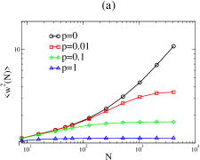
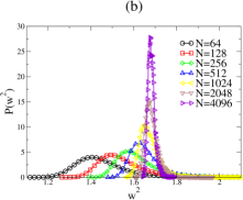
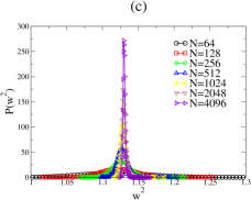
Figure 19: (a) The average steady-state width as a function of linear system size for different $p$ values in the 2D SW synchronization scheme. The data for $p$=$0$ corresponds to the 2D BCS scheme on a regular network with only nearest-neighbor connections. Steady-state width distributions in the 2D SW synchronization scheme for (b) $p$$=$$0.1$ and for (c) $p$$=$$1$ for various system sizes.

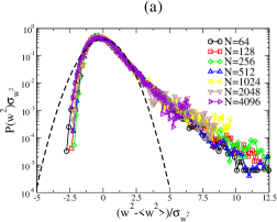
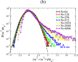
Figure 20: Steady-state width distributions in the 2D SW synchronization scheme scaled to zero mean and unit variance for (a) $p$$=$$0.1$ and for (b) $p$$=$$1$. The dashed curves are similarly scaled Gaussians for comparison.

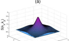
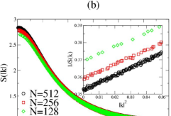
Figure 21: (a) Steady-state structure factor for the 2D SW scheme as a function of the components $k_{x}$ and $k_{y}$ for $p$$=$$1$. (b) Structure factor as a function of $|\vec{k}|$ for the 2D SW synchronization scheme for $p$=$1$. The inset shows $1/S(k)$ vs. $k^{2}$ for small values of $|k|$.

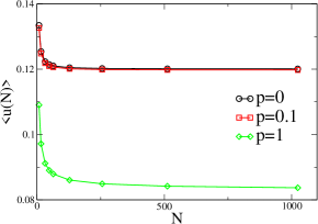
Figure 22: Steady-state utilization of SW synchronization network in 2D as a function of system-size for three different values of $p$$=$$0$ (BCS), $p$$=$$0.1$ and $p$$=$$1$.

VI Summary and Conclusions

We studied the large-scale properties of the synchronization landscapes of PDES, applicable to certain distributed and networked computer systems for a large number of scientific problems. We investigated the effects of SW-like additional communication links between the nodes added on the top of 1D and 2D regular networks. With purely regular short-range connections the synchronization landscape is rough and belongs to the KPZ universality class. This property can hinder efficient data management. To suppress diverging fluctuations (as a function of the number of the nodes) we constructed a SW synchronization scheme where the nodes also synchronize with a randomly chosen one with a possibly infinitesimal frequency. For an infinitesimally small rate of communications over the random links, this scheme results in a progress rate reduced only by an infinitesimal amount, while the width of the time horizon becomes finite in the limit of infinitely many PEs. Thus, the scheme is fully scalable as the PEs make nonzero and close-to-uniform progress without global intervention. In obtaining our results, we used coarse-grained arguments to identify the universality class of the PDES time horizon, and confirmed those predictions by actually simulating the simulations, based on the exact algorithmic rules. Our study of the width distributions of SW-synchronized PDES landscapes also revealed that while they converge to delta-functions, centered about a finite value, their shape progressively becomes non-Gaussian for larger values of $p$. We could not conclude if these observations indicate the emergence of a strong-disorder regime, or strong non-monotonic finite size effects for our attainable system sizes. Future work may address these questions.

In this work we considered the simplest (and in some regards, the worst case) scenario, where each nodes carries one site of the underlying physical system, hence synchronization with nearest neighbor PEs is required at every step. In actual parallel implementations the efficiency can be greatly increased by hosting many sites by each PE KORN99_JCP ; AMAR_PRB_2005a ; AMAR_PRB_2005b . That way, communication between PEs is only required when local variables are to be updated on the boundary region of the sites hosted by the PEs (within the finite range of the interactions). While the above procedure clearly increases the utilization and reduces the actual communication overhead, it gives rise to an even faster growing early time regime in the simulated time horizon KOLA_PRE_2004 . Since the PEs rarely need to synchronize, up to some crossover time, the evolution of the time horizon is governed by random deposition BARA95 , a faster roughening growth, before eventually crossing over to the KPZ growth and a subsequent saturation.

Our findings are also closely related to critical phenomena and collective phenomena on networks ALBERT02 ; DOROGOVTSEV02 ; STROGATZ01 ; GOLTSEV03 . In particular, in recent years, a number of prototypical models have been investigated on SW networks WATTS98 ; WATTS99 ; NEWMAN00 ; NEWMAN99 ; MONASSON99 ; SCALETT91 ; BARRAT00 ; GITTERMAN00 ; KIM01 ; PEKALSKI01 ; HONG02_1 ; HONG02_2 ; HERRERO02 ; JEONG03 ; Toral ; HASTINGS03 ; BLUMEN_2000a ; BLUMEN_2000b ; ALMAAS_2002 ; KOZMA03 ; KOZMA05 ; KOZMA05b ; HASTINGS04 . Of these, the ones most closely related to our work are the XY model KIM01 , the EW model KOZMA03 ; KOZMA05 ; KOZMA05b , diffusion MONASSON99 ; BLUMEN_2000a ; BLUMEN_2000b ; ALMAAS_2002 ; KOZMA03 ; KOZMA05 ; KOZMA05b ; HASTINGS04 , and current flow KORN_PLA_swrn on SW networks. The findings suggest that systems without inherent frustration exhibit (strict or anomalous) KOZMA03 ; KOZMA05 ; KOZMA05b ; HASTINGS03 ; HASTINGS04 mean-field-like behavior when the original short-range interaction topology is modified to a SW network. In essence, the SW couplings, although sparse, induce an effective relaxation to the mean of the respective local field variables, and in turn, the system exhibits a mean-field-like behavior HASTINGS03 . This effect is qualitatively similar to those observed in models with “annealed” long-range random couplings DRT90 ; BR91 ; BLUMEN_2000b , but on (quenched) SW networks, the scaling properties can differ from those with annealed interactions KOZMA03 ; KOZMA05 ; KOZMA05b ; HASTINGS03 ; HASTINGS04 .

- (1) R. Albert and A.-L. Barabási, Rev. Mod. Phys. 74, 47 (2002).
- (2) S.N. Dorogovtsev and J.F.F. Mendes, Adv. Phys. 51, 1079 (2002).
- (3) M.E.J. Newman, SIAM Review 45, 167 (2003).
- (4) M. Faloutsos, P. Faloutsos, and C. Faloutsos, Proc. ACM SIGCOMM, Comput. Commun. Rev. 29, 251 (1999).
- (5) A.-L. Barabási and R. Albert, Science 286, 509 (1999).
- (6) R. Albert, H. Jeong, and A.-L. Barabási, Nature 401, 130 (1999).
- (7) H. Jeong, B. Tombor, R. Albert, Z.N. Oltvai, and A.-L. Barabási, Nature 407, 651 (2000).
- (8) A. Barrat, M. Barhélemy, R. Pastor-Satorras, and A. Vespignani, Proc. Natl. Acad. Sci. USA 101, 3747 (2004).
- (9) R. Guimerá, S. Mossa, A. Turtschi, and L.A.N. Amaral, Proc. Natl. Acad. Sci. USA 102, 7794 (2005).
- (10) S. Eubank, H. Guclu, V.S.A. Kumar, M.V. Marathe, A. Srinivasan, Z. Toroczkai, and N. Wang, Nature 429, 180 (2004).
- (11) S. Milgram, Psychology Today 2, 56 (1967).
- (12) D.J. Watts and S.H. Strogatz, Nature 393, 440 (1998).
- (13) P. Erdős and A. Rényi, Publ. Math. Inst. Hung. Acad. Sci 5, 17 (1960).
- (14) R.T. Scalettar, Physica A 170 282 (1991).
- (15) M. Gitterman, J. Phys. A 33, 8373 (2000).
- (16) A. Barrat and M. Weigt, Eur. Phys. J. B 13, 547 (2000).
- (17) M.A. Novotny and S.M. Wheeler, Brazilian J. of Physics 34, 395 (2004).
- (18) B.J. Kim, H. Hong, P. Holme, G.S. Jeon, P. Minnhagen, and M.Y. Choi, Phys. Rev. E 64, 056135 (2001).
- (19) H. Hong, M.Y. Choi, and B.J. Kim, Phys. Rev. E 65, 047104 (2002).
- (20) B. Kozma, M.B. Hastings, and G. Korniss, Phys. Rev. Lett. 92, 108701 (2004).
- (21) B. Kozma, M.B. Hastings, and G. Korniss, in Noise in Complex Systems and Stochastic Dynamics III, edited by L.B. Kish, K. Lindenberg, Z. Gingl, Proceedings of SPIE Vol. 5845 (SPIE, Bellingham, WA, 2005) pp.130–138.
- (22) B. Kozma, M.B. Hastings, and G. Korniss, Phys. Rev. Lett. (in press, 2005); arXiv: cond-mat/0501509.
- (23) R. Monasson, Eur. Phys. J. B 12, 555 (1999).
- (24) S. Jespersen, I.M. Sokolov, and A. Blumen, Phys. Rev. E 62, 4405 (2002).
- (25) S. Jespersen and A. Blumen, Phys. Rev. E 62, 6270 (2002).
- (26) E. Almaas, R.V. Kulkarni, and D. Stroud, Phys. Rev. Lett. 88, 098101 (2002).
- (27) M.B. Hastings, Eur. Phys. J. B 42, 297 (2004)
- (28) G. Korniss, M.B. Hastings, K.E. Bassler, M.J. Berryman, B. Kozma, D. Abbott, Phys. Lett. A (in press, 2005); arXiv:cond-mat/0508056.
- (29) K. Wiesenfeld, P. Colet, and S.H. Strogatz, Phys. Rev. Lett. 76, 404 (1996).
- (30) S.H. Strogatz, Nature 410, 268 (2001).
- (31) M. Barahona and L.M. Pecora, Phys. Rev. Lett. 89, 054101 (2002).
- (32) H. Hong, B.J. Kim, and M.Y. Choi, Phys. Rev. E 66, 018101 (2002).
- (33) G. Korniss, Z. Toroczkai, M.A. Novotny, and P.A. Rikvold, Phys. Rev. Lett. 84, 1351 (2000).
- (34) R.M. Fujimoto, Commun. of the ACM 33, 30 (1990).
- (35) D.M. Nicol and R.M. Fujimoto, Annals of Operations Research 53 249 (1994).
- (36) B.D. Lubachevsky, Bell Labs Tech. J. 5, April-June 2000, 134 (2000).
- (37) A. Kolakowska, M. A. Novotny, in Progress in Computer Science Research (Nova Science Publishers, in press); arXiv:cs.DC/0409032 (2004).
- (38) G. Korniss, M.A. Novotny, H. Guclu, Z. Toroczkai, and P.A. Rikvold, Science 299, 677 (2003).
- (39) A.G. Greenberg, B.D. Lubachevsky, D.M. Nicol, and P.E. Wright Proceedings of the 8th Workshop on Parallel and Distributed Simulation (PADS’94), Edinburgh, UK, 1994 (SCS, San Diego, CA, 1994), 187 (1994).
- (40) G. Korniss, M.A. Novotny, and P.A. Rikvold, J. Comput. Phys. 153, 488 (1999).
- (41) G. Korniss, C.J. White, P.A. Rikvold, and M.A. Novotny, Phys. Rev. E 63, 016120 (2001).
- (42) E. Deelman, B. K. Syzmanski, and T. Caraco, Proceedings of the 28th Winter Simulation Conference (ACM, New York), 1191 (1996).
- (43) Y. Shim and J.G. Amar, Phys. Rev. B 71, 115436 (2005).
- (44) Y. Shim and J.G. Amar, Phys. Rev. B 71, 125432 (2005).
- (45) Y. Shim and J.G. Amar, J. Comput. Phys. (in press, 2005).
- (46) D.M. Nicol, Proceedings of the 1988 SCS Multiconference, Simulation Series, SCS Vol. 19, 141 (1988).
- (47) J. Cowie, D.M. Nicol and A. Ogielski, IEEE Computing in Science and Engineering 1, 42 (1999).
- (48) D.R. Jefferson, ACM Trans. Programming Languages and Systems 7, 404 (1985).
- (49) K.M. Chandy and J. Misra, IEEE Trans. on Softw. Eng. SE-5, 440 (1979).
- (50) K.M. Chandy and J. Misra, Commun. ACM 24, 198 (1981).
- (51) E. Deelman and B.K. Szymanski, Proc. of the 11th Workshop on Parallel and Distributed Simulation, PADS ’97, (IEEE Computer Society, Los Alamitos, California), 124 (1997).
- (52) C.D. Carothers, K.S. Perumalla and R.M. Fujimoto, ACM Transactions on Modeling and Computer Simulation 9, 224 (1999).
- (53) G. Chen and B.K. Szymanski, Proc. of the 16th Workshop on Parallel and Distributed Simulation, PADS ’02 (IEEE Computer Society, Los Alamitos, California), 153 (2002).
- (54) L. N. Shchur and M. A. Novotny, Phys. Rev. E 70, 026703 (2004).
- (55) See also www.top500.org and www.research.ibm.com/bluegene/.
- (56) See, e.g., www.gridforum.org and setiathome.ssl.berkeley.edu.
- (57) S. Kirkpatrick, Science 299, 668 (2003).
- (58) P.M.A. Sloot, B.J. Overeinder, and A. Schoneveld, Comput. Phys. Commun. 142, 76 (2001).
- (59) P. Bak, C. Tang, and K. Wiesenfeld, Phys. Rev. Lett. 59, 381 (1987).
- (60) P. Bak, C. Tang, and K. Wiesenfeld, Phys. Rev. A 38, 364 (1988).
- (61) G. Korniss, M.A. Novotny, Z. Toroczkai, and P.A. Rikvold, in Computer Simulation Studies in Condensed Matter Physics XIII, Springer Proceedings in Physics, Vol. 86, editors D.P. Landau, S.P. Lewis, and H.-B. Schüttler (Springer-Verlag, Berlin, Heidelberg, 2001), pp. 183–188.
- (62) Frontiers in Problem Solving: Phase Transitions and Complexity, edited by T. Hogg, B.A. Huberman, and C. Williams, Artif. Intell. 81 issue 1-2 (1996).
- (63) R. Monasson, R. Zecchina, S. Kirkpatrick, B. Selman, and L. Troyansky, Nature 400, 133 (1999).
- (64) D.M. Nicol, ACM Trans. Model. Comput. Simul. 1, 24 (1991).
- (65) R.E. Felderman and L. Kleinrock, ACM Trans. Model. Comput. Simul. 1, 386 (1991).
- (66) B.D. Lubachevsky, Complex Systems 1, 1099 (1987).
- (67) B.D. Lubachevsky, J. Comput. Phys. 75, 103 (1988).
- (68) A.-L. Barabási and H.E. Stanley, Fractal Concepts in Surface Growth, (Cambridge University Press, Cambridge, 1995).
- (69) T. Halpin-Healy and Y.-C. Zhang, Phys. Rep. 254 215 (1995).
- (70) J. Krug, Adv. Phys. 46, 139 (1997).
- (71) F. Family and T. Vicsek, J. Phys. A 18, L75 (1985).
- (72) Z. Toroczkai, G. Korniss, S. Das Sarma, and R. K. P. Zia, Phys. Rev. E 62, 276 (2000).
- (73) J. Krug and P. Meakin, J. Phys. A 23, L987 (1990).
- (74) G. Korniss, M.A. Novotny, A.K. Kolakowska, and H. Guclu, SAC 2002, Proceedings of the 2002 ACM Symposium On Applied Computing, 132 (2002).
- (75) A. Kolakowska, M.A. Novotny, and G. Korniss, Phys. Rev. E 67, 046703 (2003).
- (76) A. Kolakowska, M.A. Novotny, and P.A. Rikvold, Phys. Rev. E 68, 046705 (2003).
- (77) A. Kolakowska and M.A. Novotny, Phys. Rev. B 69, 075407 (2004).
- (78) M. Kardar, G. Parisi, and Y.-C. Zhang, Phys. Rev. Lett. 56, 889 (1986).
- (79) S.F. Edwards and D.R. Wilkinson, Proc. R. Soc. London Ser. A 381, 17 (1982).
- (80) Z. Toroczkai, G. Korniss, M.A. Novotny, and H. Guclu, in Computational Complexity and Statistical Physics, eds. A. Percus, G. Istrate, and C. Moore, Santa Fe Institute Studies in the Sciences of Complexity Series (Oxford University Press, in press); arXiv: cond-mat/0304617.
- (81) G. Foltin, K. Oerding, Z. Rácz, R.L. Workman, and R.K.P. Zia, Phys. Rev. E 50, R639 (1994).
- (82) M. Plischke, Z. Rácz, and R.K.P. Zia, Phys. Rev. E 50, 3589 (1994).
- (83) Z. Rácz and M. Plischke, Phys. Rev. E 50, 3530 (1994).
- (84) T. Antal and Z. Rácz, Phys. Rev. E 54, 2256 (1996).
- (85) T. Antal, M. Droz, G. Györgyi, and Z. Rácz, Phys. Rev. Lett 87, 240601 (2001).
- (86) T. Antal, M. Droz, G. Györgyi, and Z. Rácz, Phys. Rev. E 65, 046140 (2002).
- (87) A.G. Greenberg, S. Shenker, and A.L. Stolyar, Proc. ACM Sigmetrics Performance Eval. Rev. 24, 91 (1996).
- (88) E. Marinari, A. Pagnani, G. Parisi, and Z. Rácz, Phys. Rev. E 65, 026136 (2002).
- (89) B. Bollobas, Random Graphs (Cambridge University Press, Cambridge, 2001).
- (90) H. Guclu, G. Korniss, Z. Toroczkai, and M.A. Novotny, in Complex Networks, edited by E. Ben-Naim, H. Frauenfelder, and Z. Toroczkai, Lecture Notes in Physics Vol. 650 (Springer-Verlag, Berlin, 2004) pp. 255–275.
- (91) E. Marinari, A. Pagnani, and G. Parisi, J. Phys. A 33, 8181 (2000).
- (92) J.M. Kim and J.M. Kosterlitz, Phys. Rev. Lett. 62, 2289 (1989).
- (93) A. Kolakowska, M.A. Novotny, and P.S. Verma, Phys. Rev. E 70, 051602 (2004).
- (94) A.V. Goltsev, S.N. Dorogovtsev, and J.F.F. Mendes, Phys. Rev. E 67, 026123 (2003).
- (95) D.J. Watts, Small Worlds (Princeton Univ. Press, Princeton, 1999).
- (96) M.E.J. Newman, J. Stat. Phys. 101, 819 (2000).
- (97) M.E.J. Newman, and D.J. Watts, Phys. Lett. A 263, 341 (1999).
- (98) M.B. Hastings, Phys. Rev. Lett. 91, 098701 (2003).
- (99) C.P. Herrero, Phys. Rev. E 65, 066110 (2002).
- (100) A. Pekalski, Phys. Rev. E 64 057104 (2001).
- (101) D. Jeong, H. Hong, B. J. Kim and M. Y. Choi, Phys. Rev. E 68 027101 (2003).
- (102) J. Viana Lopes, Y.G. Pogorelov, J.M.B. Lopes dos Santos, and R. Toral Phys. Rev. E 70, 026112 (2004).
- (103) M. Droz, Z. Rácz, and P. Tartaglia, Phys. Rev. A 41 6621 (1990).
- (104) B. Bergersen and Z. Rácz, Phys. Rev. Lett. 67 3047 (1991).