Ginzburg-Landau theory of crystalline anisotropy for bcc-liquid interfaces

Abstract

The weak anisotropy of the interfacial free-energy $\gamma$ is a crucial parameter influencing dendritic crystal growth morphologies in systems with atomically rough solid-liquid interfaces. The physical origin and quantitative prediction of this anisotropy are investigated for body-centered-cubic (bcc) forming systems using a Ginzburg-Landau theory where the order parameters are the amplitudes of density waves corresponding to principal reciprocal lattice vectors. We find that this theory predicts the correct sign, $\gamma_{100}>\gamma_{110}$, and magnitude, $(\gamma_{100}-\gamma_{110})/(\gamma_{100}+\gamma_{110})\approx 1\%$, of this anisotropy in good agreement with the results of MD simulations for Fe. The results show that the directional dependence of the rate of spatial decay of solid density waves into the liquid, imposed by the crystal structure, is a main determinant of anisotropy. This directional dependence is validated by MD computations of density wave profiles for different reciprocal lattice vectors for $\{110\}$ crystal faces. Our results are contrasted with the prediction of the reverse ordering $\gamma_{100}<\gamma_{110}$ from an earlier formulation of Ginzburg-Landau theory [Shih et al., Phys. Rev. A 35, 2611 (1987)].

I Introduction

The advent of microscopic solvability theory Langer ; KesslerAP ; Amar in the 1980s lead to the prediction that the anisotropy of the excess free-energy of the crystal-melt interface is a crucial parameter that determines the growth rate and morphology of dendrites, which shape the microstructures of many commercial metallic alloys. This prediction was largely validated by phase-field simulations KarmaRappelII ; Provatas of dendritic solidification during the 1990s. More recent work in the present decade has focused on the quantitative prediction of both the magnitude and the anisotropy of the interfacial free-energy $\gamma$ using molecular dynamics (MD) simulations broughton86 ; davidchack00 ; davidchack03 ; davidchack05 ; hoyt01 ; hoyt02 ; hoyt03 ; asta02 ; morris02 ; morris03 ; sun04 ; sun041 ; sun05 ; laird05 ; hoyt06 ; song05 ; davidchack06 . In parallel, experimental progress has been made to determine this anisotropy in metallic systems from accurate equilibrium shape measurements napolitano ; liu01 ; napolitano04 , which extend pioneering measurements of this anisotropy in transparent organic crystals Huang ; glicksman .

MD-based methods, including the cleaving technique broughton86 ; davidchack00 ; davidchack03 ; davidchack05 and the capillary fluctuation method (CFM) hoyt01 ; morris02 , have been successfully developed to compute $\gamma$ and to accurately resolve its notoriously small anisotropy of the order of $1\%$. These methods have been applied to a wide range of systems, including several elemental face-centered-cubic (fcc) hoyt01 ; hoyt02 ; morris02 ; sun04 ; sun041 , body-centered-cubic (bcc) sun04 ; sun041 ; hoyt06 , and hexagonal-close-packed sun05 metals, as well as one fcc metallic alloy asta02 modeled with interatomic potentials derived from the embedded-atom-method (EAM), the Lennard-Jones system davidchack03 ; morris03 , hard-sphere davidchack00 ; song05 ; davidchack06 and repulsive power-law potentials davidchack05 , and, most recently, a bcc molecular organic succinonitrile laird05 used extensively in experimental studies of crystal growth patterns.

In systems with an underlying cubic symmetry, the magnitude of the crystalline anisotropy has been traditionally characterized by comparing the values of $\gamma$ corresponding to $\{100\}$ and $\{110\}$ crystal faces. MD calculations have yielded anisotropy values $(\gamma_{100}-\gamma_{110})/(\gamma_{100}+\gamma_{110})=0.5-2.5\%$, and experimental values extracted from equilibrium shape measurements fall generally within this range. What determines physically the positive sign and the magnitude of this anisotropy, however, remains unclear. One interesting clue is that MD-calculated anisotropies generally depend more on the crystal structure than on the microscopic details of inter-molecular forces for the same crystal structure, and anisotropies tend to be consistently smaller for bcc than for fcc hoyt06 . A striking example of the former is the fact that MD studies of Fe sun04 ; sun041 and succninonitrile laird05 , with the same bcc structure but entirely different inter-molecular forces, have yielded comparable anisotropies around half a percent. The weaker anisotropy of $\gamma$ for bcc compared to fcc is also consistent with experimental measurements of anisotropy values in the range of $0.5-0.7\%$ and $2.5-5\%$ for the bcc and fcc transparent organic crystals succinonitrile and pivalic acid, respectively glicksman ; muschol .

The fact that anisotropy appears to depend more strongly on crystal structure than inter-molecular forces suggests that it may be possible to predict this critical parameter from a continuum density wave description of the solid-liquid interface, which naturally incorporates anisotropy because of the broken symmetry of the solid. The simplest of such descriptions is the Ginzburg-Landau (GL) theory of the bcc-liquid interface developed by Shih et al. Shih . The order parameters of this theory are the amplitudes of density waves corresponding to the set of principal reciprocal lattice vectors $\{\vec{K}_{i}\}$, and the free-energy functional is derived from density functional theory (DFT) RY ; HOI ; HOII with certain simplifying assumptions.

This theory has yielded predictions of $\gamma$ for various bcc elements that are in reasonably good agreement with experiments. Moreover, it has provided an elegant analytical derivation of the proportionality between $\gamma$ and the latent heat of fusion, in agreement with the scaling relation $\gamma n^{-2/3}=\alpha L$ proposed by Turnbull Turnbull and recently corroborated by MD simulations sun04 ; davidchack05 , where $n$ is the solid atomic density and $L$ is the latent hear per atom. This theory, however, predicts the wrong ordering $\gamma_{100}<\gamma_{110}$. This apparent failure could be due to the truncation of larger $|\vec{K}|$ modes, i.e. density waves corresponding to reciprocal lattice vectors $\vec{K}$ with $|\vec{K}|>|\vec{K}_{i}|$. However, paradoxically, a strong dependence of the anisotropy on larger $\vec{K}$ modes would be hard to reconcile with the weak dependence of this quantity on details of inter-molecular forces seen in MD studies, since these forces dictate the amplitudes of these modes in the crystal where the density is sharply peaked around atomic positions.

To shed light on this paradox, we revisit the simplest GL theory of the bcc-liquid interface based on the minimal set of principal reciprocal lattice vectors. Our calculation differs principally from the one of Shih et al. Shih in the derivation of the coefficients of the gradient square terms in the GL free-energy functional. Each term measures the free-energy cost associated with the spatial variation, in the direction $\hat{n}$ normal to the solid-liquid interface, of a subset of equivalent density waves with the same magnitude of the direction cosine $\hat{K}_{i}\cdot\hat{n}$ and hence the same amplitude. Shih et al. choose these coefficients to be proportional to the number of principal reciprocal lattice vectors in each subset. This procedure, however, turns out to yield an incorrect directional dependence (i.e. dependence on $\hat{K}_{i}\cdot\hat{n}$) of the rate of decay of density waves into the liquid. Here we find that the inclusion of the correct directional dependence, as prescribed by DFT, yields the correct ordering $\gamma_{100}>\gamma_{110}$ and a reasonable estimate of the magnitude of anisotropy. Furthermore, we validate this directional dependence by MD computations of density wave profiles.

II Ginzburg-Landau theory

We review the derivation of the GL theory and compare our results to MD simulations in the next section. The theory is derived in the DFT framework where the free energy of an inhomogeneous system is expressed as a functional $F=F[n(\vec{r})]$ of its density distribution $n(\vec{r})$, which can be expanded in the form

$$n(\vec{r})=n_{0}\left(1+\sum_{i}u_{i}(\vec{r})\,\,e^{i\vec{K}_{i}\cdot\vec{r}}+\dots\right)$$ (1)

where the order parameters $u_{i}$’s are the amplitudes of density waves corresponding to principle lattice vectors $\langle 110\rangle$ of the reciprocal fcc lattice, and the contribution of larger $\vec{K}$ mode denoted by $``\dots"$ is neglected. Expanding the free-energy as a power series of the $u_{i}$’s around its liquid value $F_{l}\equiv F[n_{0}]$ yields

$$\Delta F = {n_{0}k_{B}T\over 2}\left(\int d\vec{r}\,a_{2}\sum_{i,j}c_{ij}\,u_{i}\,u_{j}\,\,\delta_{0,\vec{K}_{i}+\vec{K}_{j}}\right.$$

$$-a_{3} \sum_{i,j,k}c_{ijk}\,u_{i}\,u_{j}\,u_{k}\,\,\delta_{0,\vec{K}_{i}+\vec{K}_{j}+\vec{K}_{k}}$$

$$+a_{4} \sum_{i,j,k,l}c_{ijkl}\,u_{i}\,u_{j}\,u_{k}\,u_{l}\,\,\delta_{0,\vec{K}_{i}+\vec{K}_{j}+\vec{K}_{k}+\vec{K}_{l}}$$

$$+b \left.\sum_{i}c_{i}\,\left|{du_{i}\over dz}\right|^{2}\right),$$

where we have defined $\Delta F\equiv F-F_{l}$ and the gradient square terms arise from the spatial variation of the order parameters along the direction normal to the interface parameterized by the coordinate $z$. The Kronecker delta $\delta_{m,n}$, which equals $0$ or $1$ for $m\neq n$ or $m=n$, respectively, enforces that only combinations of principal reciprocal lattice vectors that form closed polygons $\vec{K}_{i}+\vec{K}_{j}+\dots=0$ contribute to the free-energy functional. Closed triangles generate a non-vanishing cubic term that makes the bcc-liquid freezing transition first order. The multiplicative factors $a_{i}$ and $b$ are introduced since it is convenient to normalize the sums of the $c$’s to unity (i.e. $\sum_{i}c_{i}=1$, $\sum_{i,j}c_{ij}\delta_{0,\vec{K}_{i}+\vec{K}_{j}}=1$, etc). To complete the theory, one needs to determine all the coefficients appearing in the GL free energy functional.

The coefficients of the quadratic terms are obtained from the standard expression for the free-energy functional that describes small density fluctuations of an inhomogeneous liquid

$$\Delta F={k_{B}T\over 2}\int\int d\vec{r}d\vec{r}^{\prime}\delta n(\vec{r})\left[{\delta(\vec{r}-\vec{r}^{\prime})\over n_{0}}-C(|\vec{r}-\vec{r}^{\prime}|)\right]\delta n(\vec{r}^{\prime})$$ (3)

where $\delta n(\vec{r})\equiv n(\vec{r})-n_{0}$ and $C(|\vec{r}-\vec{r}^{\prime}|)$ is the direct correlation function whose fourier transform

$$C(K)=n_{0}\int d\vec{r}\,C(|\vec{r}|)e^{-i\vec{K}\cdot\vec{r}}$$ (4)

is related to the structure factor $S(K)=\left[1-C(K)\right]^{-1}$.

The two expressions for $\Delta F$, Eqs. (II) and (3), can now be related by assuming that the amplitudes of density waves vary slowly across the interface on a scale $\sim 1/K_{max}$ where $K_{max}$ is the value of $K$ corresponding to the peak of the structure factor. Accordingly, $u_{i}(z^{\prime})$ can be expanded in a Taylor series about $z$

$$\delta n(\vec{r}^{\prime}) \approx n_{0}\sum_{i}\left[u_{i}(z)+{du_{i}(z)\over dz}(z^{\prime}-z)\right.$$ (5)

$$\left.+{1\over 2}{d^{2}u_{i}(z)\over dz^{2}}(z^{\prime}-z)^{2}+\dots\right]e^{i\vec{K}_{i}\cdot\vec{r}^{\prime}},$$

where the contribution $``\dots"$ involving higher-order derivatives can be neglected. Namely, terms proportional to $(z^{\prime}-z)^{n}d^{n}u_{i}(z)/dz^{n}\sim 1/(K_{max}w)^{n}$, where $w$ is the characteristic width of the solid-liquid interface, i.e. the scale over which order parameters vary from a constant value in the solid to zero in the liquid. Hence, these terms vanish at large $n$ under the assumption that $w\gg 1/K_{max}$. Substituting this expression in Eq. (3) and carrying out the integral over $\vec{r}^{\prime}$, we obtain

$$\Delta F \approx {n_{0}k_{B}T\over 2}\int d\vec{r}\left[\sum_{i,j}{1\over S(|\vec{K}_{i}|)}u_{i}u_{j}\delta_{0,\vec{K}_{i}+\vec{K}_{j}}\right.$$ (6)

$$\left.-\sum_{i}{1\over 2}C^{\prime\prime}(|\vec{K}_{i}|)(\hat{K}_{i}\cdot\hat{n})^{2}\left|{du_{i}\over dz}\right|^{2}\right],$$

where $C^{\prime\prime}(K)\equiv d^{2}C(K)/dK^{2}$. Comparing Eqs. (6) and (II), we obtain at once

$$a_{2}\,c_{ij}={1\over S(|\vec{K}_{110}|)},$$ (7)

$$b\,c_{i}=-{1\over 2}C^{\prime\prime}(|\vec{K}_{110}|)(\hat{K}_{i}\cdot\hat{n})^{2},$$ (8)

where we have used the fact that all reciprocal lattice vectors have the same magnitude $|\vec{K}_{i}|=|\vec{K}_{110}|$. Summing both sides of Eq. (7) and using the normalization $\sum_{i,j}c_{ij}\delta_{0,\vec{K}_{i}+\vec{K}_{j}}=1$ gives

$$a_{2}=\sum_{i,j}\frac{\delta_{0,\vec{K}_{i}+\vec{K}_{j}}}{S(|\vec{K}_{110}|)}={12\over S(|\vec{K}_{110}|)},$$ (9)

and $c_{ij}=1/12$. Similarly, summing over $i$ both sides of Eq. (8), and using the normalization $\sum_{i}c_{i}=1$, yields

$$b=-{1\over 2}\sum_{i}C^{\prime\prime}(|\vec{K}_{110}|)(\hat{K}_{i}\cdot\hat{n})^{2}=-\,2\,C^{\prime\prime}(|\vec{K}_{110}|),$$ (10)

where the second equality can be shown to be independent of the direction of $\hat{n}$, and

$$c_{i}={1\over 4}(\hat{K}_{i}\cdot\hat{n})^{2}$$ (11)

To make the difference between the above derivation of the $c_{i}$’s and the one of Shih et al. explicit, consider one of the $\{110\}$ crystal faces with $\hat{n}$ pointing in the $[110]$ direction. The set of 12 principal reciprocal lattice vectors $\{\vec{K}_{i}\}$ corresponding to the $\langle 110\rangle$ directions can be separated into three subsets with the same value of $(\hat{K}_{i}\cdot\hat{n})^{2}$: subset I with 8 vectors ($[011],[0\bar{1}1],[01\bar{1}],[101],[\bar{1}01],[10\bar{1}],[0\bar{1}\bar{1}],[\bar{1}0\bar{1}]$) and $(\hat{K}_{i}\cdot\hat{n})^{2}=1/4$, subset II with 2 vectors ($[110],[\bar{1}\bar{1}0]$) and $(\hat{K}_{i}\cdot\hat{n})^{2}=1$, and subset III with 2 vectors ($\bar{1}10$, $[1\bar{1}0]$) and $(\hat{K}_{i}\cdot\hat{n})^{2}=0$. Density waves in a given subset have the same amplitude denoted here by $u$, $v$, and $w$ for subsets I, II and III, respectively.

It follows that the correct coefficient of the gradient square terms for a given order parameter $u$, $v$, or $w$, is obtained using the expression for $c_{i}$ given by Eq. (11) with the corresponding value of $(\hat{K}_{i}\cdot\hat{n})^{2}$ for the corresponding subset I, II, or III, respectively. These coefficients are $c_{i}=1/16$ for subset I, $c_{i}=1/4$ for subset II, and $c_{i}=0$ for subset III. These coefficients yield the gradient square terms $-C^{\prime\prime}(|\vec{K}_{110}|)|du/dz|^{2}$ and $-C^{\prime\prime}(|\vec{K}_{110}|)|dv/dz|^{2}$ in the GL free energy functional (II) since there are $8$ equivalent reciprocal lattice vectors in subset I and $2$ in subset II, respectively. The coefficient of $|dw/dz|^{2}$ vanishes since principal reciprocal lattice vectors in subset III are orthogonal to $\hat{n}$ and $c_{i}=0$.

In contrast, Shih et al. choose the $c_{i}$’s to be equal for all subsets with a non-vanishing direction cosine (subsets I and II), and $c_{i}=0$ for subsets with principal reciprocal lattice vectors orthogonal to $\hat{n}$ (subset III). Since there is a total of 10 reciprocal lattice vectors in subsets I and II, the normalization condition $\sum_{i}c_{i}=1$ yields $c_{i}=1/10$. These coefficients yield the gradient square terms $-(8/5)C^{\prime\prime}(|\vec{K}_{110}|)|du/dz|^{2}$ and $-(2/5)C^{\prime\prime}(|\vec{K}_{110}|)|dv/dz|^{2}$ in the GL free energy functional (II), which are weighted proportionally to the number of reciprocal lattice vectors in each subset, and differ from the correct terms derived above.

For the $\{100\}$ and $\{111\}$ crystal faces, the weighting procedure of Shih et al. and Eq. (11) give coincidentally the same coefficients of the gradient square terms. Thus these cases need not be repeated here. The results for the different crystal faces are summarized in Table 1.

Table 1: Comparison of coefficients of square gradient terms $c_{i}$ predicted by Eq. (11) (DFT) and Shih et al. Shih for the $\{100\}$, $\{110\}$, and $\{111\}$ crystal faces. For each orientation, the 12 principal reciprocal lattice vector are grouped into subsets where $\hat{K}_{i}\cdot\hat{n}$ have the same magnitude in each subset.

	$100$		$110$			$111$
$(\hat{K}_{i}\cdot\hat{n})^{2}$	0	1/2	1/4	1	0	0	2/3
Number of $\vec{K}_{i}$’s	4	8	8	2	2	6	6
$c_{i}$ (Eq. 11)	0	1/8	1/16	1/4	0	0	1/6
$c_{i}$ (Ref. Shih )	0	1/8	1/10	1/10	0	0	1/6

The determination of all the other coefficients in the GL free energy functional is identical to the calculation of Shih et al.. The coefficients of the cubic and quartic terms, $c_{ijk}$ and $c_{ijkl}$, respectively, are determined by the ansatz that all polygons with the same number of sides have the same weight, which yields $c_{ijk}=1/8$ and $c_{ijkl}=1/27$; for quadratic terms, this ansatz reproduces the result $c_{ij}=1/12$ derived above since there are twelve two-sided polygons formed by the principle reciprocal lattice vectors. Using these coefficients and identifying each $u_{i}$ with the order parameter $u$, $v$, or $w$, depending on whether the corresponding ${\vec{K}_{i}}$ on one side of a polygon belongs to subset I, II, or III, respectively, Eq. (II) reduces for $\{110\}$ crystal faces to

$${\Delta F} = {n_{0}k_{B}T\over 2}\int d\vec{r}\left[a_{2}\left({2\over 3}u^{2}+{1\over 6}v^{2}+{1\over 6}w^{2}\right)\right.$$ (12)

$$-a_{3} \left({1\over 2}u^{2}v+{1\over 2}u^{2}w\right)+a_{4}\left({12\over 27}u^{4}+{1\over 27}v^{4}+{1\over 27}w^{4}\right.$$

$$\left.+{4\over 27}u^{2}v^{2}+{4\over 27}u^{2}w^{2}+{1\over 27}w^{2}v^{2}+{4\over 27}u^{2}vw\right)$$

$$\left.-C^{\prime\prime}(|\vec{K}_{110}|)\left|{du\over dz}\right|^{2}-C^{\prime\prime}(|\vec{K}_{110}|)\left|{dv\over dz}\right|^{2}\right],$$

The corresponding expression of Shih et al. differs by the coefficients of $|du/dz|^{2}$ and $|dv/dz|^{2}$ that have an extra multiplicative factor of $8/5$ and $2/5$, respectively, as discussed above. Their expressions for $\Delta F$ for the $\{100\}$ and $\{111\}$ crystal faces are identical to ours since Eq. (11) and the equal weight ansatz yield coincidentally the same $c_{i}$’s for these faces.

Finally, the coefficients $a_{3}$ and $a_{4}$ are determined by the constraints that the equilibrium state of the solid is a minimum of free energy, $\partial\Delta F/\partial u_{i}|_{u_{i}=u_{s}}$ = 0, where $u_{s}$ is the value of all the order parameters in the solid, and that solid and liquid have equal free energy at the melting point, $\Delta F(u_{s})=0$. These two constraints yield the relations $a_{3}=2a_{2}/u_{s}$ and $a_{4}=a_{2}/u_{s}^{2}$ that determine $a_{3}$ and $a_{4}$ in terms of $a_{2}$ given by Eq. (9), which completes the determination of all the coefficients.

III Results and comparison with MD simulations

The order parameter profiles for $\{110\}$ crystal faces were calculated by minimizing $\Delta F$ given by Eq. (12) with respect to the order parameters $u$, $v$ and $w$, and by solving numerically the resulting set of coupled ordinary differential equations with the boundary condition $u=v=w=u_{s}$ in solid and $u=v=w=0$ in liquid. The value of $\gamma_{110}$ was computed using Eq. (12) with these profiles. The same procedure was repeated for the $\{100\}$ and $\{111\}$ crystal faces.

We used input parameters for the GL theory computed directly from the MD simulations in order to make the comparison with these simulations as quantitative and precise as possible. These parameters include the peak of the liquid structure factor $\approx S(|\vec{K}_{110}|)$, which yields $a_{2}=3.99$ using Eq. (9), $C^{\prime\prime}(|\vec{K}_{110}|)=-10.40\,\,{\AA}^{2}$, and the amplitude of density waves corresponding to principal reciprocal lattice vectors in the solid $u_{s}=0.72$.

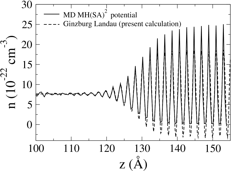
Figure 1: Comparison of planar density profiles $n(z)$ from MD simulations (solid line) and the present Ginzburg-Landau theory (dashed line) for $\{110\}$ crystal faces.

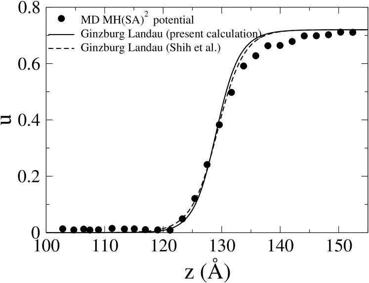
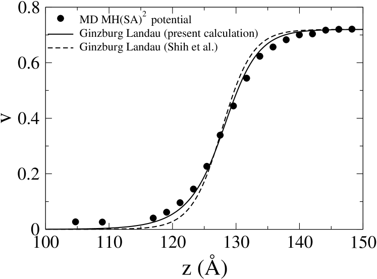
Figure 2: Comparison of numerically calculated nonlinear order parameter profiles $u$ and $v$ for $(110)$ crystal faces obtained from the present GL theory (solid line) and the GL theory of Shih et al. Shih (dashed line) and computed form MD simulations using Eq. (14) with $\vec{K}_{101}$ and $\vec{K}_{110}$ for $u$ and $v$, respectively (solid circles).

Table 2: Comparison of interfacial free energies for different crystal faces (in erg/cm²) and anisotropy parameter $\epsilon_{4}\equiv(\gamma_{100}-\gamma_{110})/(\gamma_{100}+\gamma_{110})$ predicted by Ginzburg-Landau theory with input parameters from MD simulations for Fe with the EAM potential of MH(SA)² MHSA2 (Table 3), and obtained from MD with the MH(SA)² potential and two other potentials.

	$100$	$110$	$111$	$\epsilon_{4}(\%)$
MD (ABCH) (Ref. sun04 )	207.3 (10.1)	205.7 (10.0)	205.0 (10.0)	0.4(0.4)
MD (Pair) (Ref. sun04 )	222.5 (14.1)	220.2 (14.0)	220.8 (14.0)	0.5(0.5)
MD (MH(SA)2) (Ref. sun04 )	177.0 (10.8)	173.5 (10.6)	173.4 (10.6)	1.0(0.6)
GL (present calculation)	144.26	141.35	137.57	1.02
GL (Shih et al. Shih )	144.26	145.59	137.57	$-$0.46

The MD simulations were carried out using the EAM potential for Fe from Mendelev, Han, Srolovitz, Ackland, Sun and Asta (MH(SA)²) MHSA2 and the same thermodynamic ensemble and geometries as in Ref. sun041 , which need not be repeated here. The main difference of the present simulations is the way in which the MD results were used to calculate density wave profiles. In Ref. sun041 , the amplitudes were computed by averaging over many configurations the instantaneous value of a planar structure function (i.e., the magnitude of the complex Fourier coefficients of the density). With this approach the amplitudes of density waves saturate to a small non-vanishing value in the liquid. These amplitudes, however, are generally expected to vanish in the liquid that has no long range order, consistent with the GL theory.

To calculate amplitudes that vanish in the liquid, the following procedure is followed. We first compute the average number density $n(\vec{r})=n(x,y,z)$, with $z$ measured from a fixed reference plane of atoms in the solid. During the MD simulations, only those configurations where the solid-liquid interface has the same average position along $z$ were considered. As described in detail by Davidchack and Laird, Davidchack98 this procedure avoids an artifical broadening of the density profiles due to either the natural fluctuations in the average position of the interface or Brownian motion of the crystal. The interface position is found by first assigning to each atom an order parameter proportional to the mean square displacement of atoms from their positions on a perfect bcc lattice. (The order parameter calculation is the same as that used in the capillary fluctuation method and is described in more detail in reference sun04 ). Then an order parameter profile as a function of $z$ is computed by averaging within the $x-y$ plane and the interface position is that value of $z$ where the averaged order parameter is midway between the bulk liquid and bulk solid values.

Next, we compute the $x-y$ averaged density

$$n(z)=\frac{1}{L_{x}L_{y}}\int_{0}^{L_{x}}\int_{0}^{L_{y}}dxdy\,n(\vec{r}),$$ (13)

which is illustrated in Fig. 1. Lastly, we calculate the amplitude of density waves from the fourier transform

$$u_{i}=\frac{1}{L_{x}L_{y}\Delta z}\int_{0}^{L_{x}}\int_{0}^{L_{y}}\int_{z_{j}}^{z_{j+1}}dxdydz\,n(\vec{r})\exp(i\vec{K}_{i}\cdot\vec{r}),$$ (14)

where $z_{j}$ and $z_{j+1}$ correspond to sequential minima of $n(z)$ and $\Delta z\equiv z_{j+1}-z_{j}$. In addition, $u_{i}$ is evaluated at the midpoint of this interval, $(z_{j}+z_{j+1})/2$. The order parameters $u$ and $v$ were computed for $\{110\}$ crystal faces using $\vec{K}_{110}$ and $\vec{K}_{101}$, respectively.

The results of the present GL theory are compared to those of Shih et al. and MD simulations in Fig. 2 and Table 2. Using Eq. (12) with the $c_{i}$’s given by Eq. (11), we obtain the correct ordering of interfacial free energies $\gamma_{100}>\gamma_{110}$ and a weak capillary anisotropy $(\gamma_{100}-\gamma_{110})/(\gamma_{100}+\gamma_{110})\approx 1\%$, consistent with the results of MD simulations for bcc elements davidchack05 ; sun04 ; sun041 ; laird05 ; hoyt06 , while the ansatz of equally weighted $c_{i}$’s of Shih et al. (with the values listed in Table 1) gives the reversed ordering $\gamma_{100}<\gamma_{110}$. Note that the predictions of GL theory are to be compared to the MD results with the MH(SA)² potential in Table 2 since this potential is used here to compute input parameters for this theory given in Table 3. MD results for the other potentials are mainly included to illustrate the dependence of $\gamma$ and its anisotropy on details of interatomic forces.

Fig. 1 shows that the planar density profile predicted by GL theory, obtained by substituting Eq. (1) with the numerically calculated order parameter profiles into Eq. (13), is in remarkably good agreement with MD simulations on the liquid side. The discrepancy on the solid side is due to the fact that GL theory neglects the contribution of larger $|\vec{K}|$ reciprocal lattice vectors that contribute to the localization of density peaks around bcc lattice positions in MD simulation.

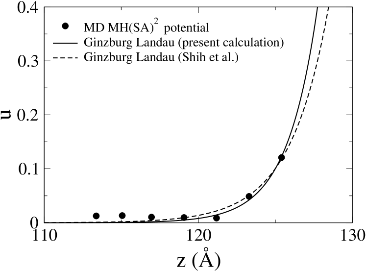
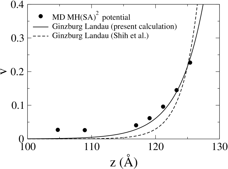
Figure 3: Comparison of analytically calculated linearized order parameter profiles $u$ and $v$ for $(110)$ crystal faces near the liquid from the present GL theory (solid line) and the GL theory of Shih et al. Shih (dashed line), and computed from MD simulations using Eq. (14) with $\vec{K}_{101}$ and $\vec{K}_{110}$ for $u$ and $v$, respectively (solid circles).

Fig. 2 shows that the amplitude profiles and the interface widths predicted by GL theory are in good agreement with MD simulations. The MD results clearly validate the directional dependence of the rate of spatial decay of density waves in the liquid that is the main determinant of the anisotropy of $\gamma$. This directional dependence is most clearly seen by examining the amplitude profiles on the liquid side of the interface. In this region, the amplitudes of density waves are sufficiently small that one can neglect the cubic and quartic terms in the GL free energy functional. The resulting linear second order differential equations for $u$ and $v$ obtained by minimizing this functional can be solved analytically, and have exponentially decaying solutions that are compared to the MD results in Fig. 3. The coefficients of the gradient square terms in the free energy functional control the decay rates. The $u$ and $v$ profiles (i.e. the amplitude of density waves corresponding to $\vec{K}_{101}$ and $\vec{K}_{110}$) calculated with coefficients that depend on the angle between the principal reciprocal lattice vectors and the interface normal through Eq. (11), which is consistent with DFT, have different decay rates that are in good quantitative agreement with the MD results. In contrast, $u$ and $v$ profiles calculated based on the ansatz of equal weights for the $c_{i}$’s Shih have the same spatial decay rate, which does not agree with the MD results.

It is interesting to note that Mikheev and Chernov (MC) MC1 ; MC2 , in a formulation of the anisotropy of the solid-liquid interface $mobility$, also stress the importance of the decay rate of the amplitude of density waves. The MC model predicts crystal growth rates and anisotropies that are in qualitative agreement with MD simulations of FCC systems. The theory, however, is linear in the sense that only the effective widths of the density profiles, which are allowed to vary with $\vec{K}$ and $\hat{n}$, are required and the authors make no attempt to compute, as was done here, the full amplitude profile as a function of $z$.

Finally, even though we have focused primarily in this paper on crystalline anisotropy, it is useful to re-examine the prediction of GL theory for the magnitude of $\gamma$ and for the Turnbull coefficient using input parameters from the present MD simulations. Shih et al. Shih derived an analytical expression for the magnitude of $\gamma$ in the isotropic approximation where all the order parameters are assumed to have the same profile through the interface, i.e. $u_{i}(z)=u$ for all $i$. In this approximation, the free energy density reduces to the sum of the gradient square term $b|du/dz|^{2}$ and a quartic polynomial in $u$. The stationary profile $u(z)$ that minimizes the free energy is then an exact hyperbolic tangent profile and the analytical expression for the interfacial energy is

$$\gamma={n_{0}k_{B}T_{m}\over 6}u_{s}^{2}(a_{2}b)^{1/2}.$$ (15)

Furthermore, Shih et al. related the latent heat (per atom) to the temperature variation of the inverse of the peak of structure factor proportional to $a_{2}$ (Eq. 9),

$$L={T_{m}\over N}\left.{\partial\Delta F\over\partial T}\right|_{T=T_{m}}={k_{B}T_{m}^{2}\over 2}u_{s}^{2}\left.\frac{da_{2}}{dT}\right|_{T=T_{m}}$$ (16)

where $N$ is the number of atoms in the system. This yields the expression for the Turbull coefficient

$$\alpha=\frac{\gamma n_{0}^{-2/3}}{L}=\frac{n_{0}^{1/3}(a_{2}b)^{1/2}}{3T_{m}\left.da_{2}/dT\right|_{T=T_{m}}},$$ (17)

which Shih et al. evaluate using parameters for the hard sphere system Shih . Using the values of the various coefficients obtained from MD simulations listed in table 3, Eq. (15) yields a value of $\gamma=147.4$ erg/cm² in reasonably good agreement with the average values of $\gamma$ for the different crystal faces in Table 2 obtained from MD simulations and the fully anisotropic GL calculation with different order parameter profiles. With the same coefficients, Eq. (16) yields a latent heat value $L=0.114$ eV/atom about 30% lower than the MD value in Table 3, where the difference can be attributed to the contribution of larger $\vec{K}$ modes that are neglected in GL theory. Eq. (17) in turn predicts a value of the Turnbull coefficient $\alpha=0.45$ that is about 25% larger than the MD value $\alpha\approx 0.36$, owing to the underestimation of the latent heat of melting in GL theory with input parameters of Table 3 from the present MD simulations. In the future, it would be interesting to test how the Turbull coefficient predicted by GL theory (Eq. 17) varies with input parameters computed from MD simulations using different interatomic potentials.

Table 3: Values of input coefficients for Ginzburg-Landau theory computed from MD simulations using the EAM potential for Fe from MH(SA)² MHSA2 and average value of $\gamma$ and latent heat of melting from these simulations.

	$a_{2}$	$b$ (${\AA}^{2}$)	$da_{2}/dT$ (K-1)	$u_{s}$	$\gamma$ (erg/cm2)	$L$ (eV/atom)
MD (MH(SA)2)	3.99	20.81	0.00163	0.72	175(11)	0.162

IV Conclusions

We have revisited the simplest GL theory of the bcc-liquid interface whose order parameters are the amplitudes of density waves corresponding to principle reciprocal lattice vectors. We find that, despite its simplicity, this theory is able to predict the density wave structure of the interface and the anisotropy of the interfacial energy, in reasonably good quantitative agreement with the results of MD simulations.

A main determinant of the anisotropy of the interfacial energy in this theory is the rate of spatial decay of density waves in the liquid. This decay rate must depend on the angle between principal reciprocal lattice vectors and the direction normal to the interface for this theory to be consistent with DFT. This directional dependence, which we validated quantitatively by MD simulations, is a direct reflection of the underlying crystal structure. Therefore, the present results provide a simple physical picture of the strong relationship between crystal structure and crystalline anisotropy, consistent with the findings of a growing body of MD-based and experimental studies of crystalline anisotropy.

An interesting future prospect is to extend the GL theory to other crystal structures, and in particular fcc-liquid interfaces. This requires, however, to consider the coupling of density waves corresponding to the principal reciprocal lattice vectors to larger $\vec{K}$ modes, which makes the theory intrinsically more complicated.

- (1) J. S. Langer, in Chance and Matter, Lectures on the Theory of Pattern Formation, Les Houches, Session XLVI, edited by J. Souletie, J. Vannimenus, and R. Stora (North-Holland, Amsterdam, 1987), pp. 629-711.
- (2) D. Kessler, J. Koplik, and H. Levine, Adv. Phys. 37, 255 (1988).
- (3) M. Ben Amar and E. Brener, Phys. Rev. Lett. 71, 589 (1993).
- (4) A. Karma and W. J. Rappel, Phys. Rev. Lett. 77, 4050 (1996); Phys. Rev. E 57, 4323 (1998).
- (5) N. Provatas, N. Goldenfeld, and J. Dantzig, Phys. Rev. Lett. 80, 3308 (1998).
- (6) J. Q. Broughton and G. H. Gilmer, J. Chem. Phys. 84, 5759 (1986).
- (7) R. L. Davidchack and B. B. Laird, Phys. Rev. Lett. 85, 4751 (2000).
- (8) R. L. Davidchack and B. B. Laird, J. Chem. Phys. 118, 7651 (2003).
- (9) R. L. Davidchack and B. B. Laird, Phys. Rev. Lett. 94, 086102 (2005).
- (10) J. J. Hoyt, M. Asta and A. Karma, Phys. Rev. Lett. 86, 5530 (2001).
- (11) J. J. Hoyt and M. Asta, Phys. Rev. B 65, 214106 (2002).
- (12) J. J. Hoyt, M. Asta and A. Karma, Mat. Sci. Engin. R 41, 121 (2003).
- (13) M. Asta, J. J. Hoyt and A. Karma, Phys. Rev. B 66, 100101(R) (2002).
- (14) J. R. Morris, Phys. Rev. B 66, 144104 (2002).
- (15) J. R. Morris and X. Y. Song, J. Chem. Phys. 119, 3920 (2003).
- (16) D. Y. Sun, M. Asta, J. J. Hoyt, M. I. Mendelev and D. J. Srolovitz, Phys. Rev. B 69, 020102(R) (2004).
- (17) D. Y. Sun, M. Asta and J. J. Hoyt, Phys. Rev. B 69, 174103 (2004).
- (18) D. Y. Sun, M. I. Mendelev, C. Becker, M. Asta, K. Kudin, D. J. Srolovitz, J. J. Hoyt, T. Haxhimali and A. Karma, Phys. Rev. B (submitted).
- (19) X. Feng and B. B. Laird, J. Chem. Phys. (submitted).
- (20) J. J. Hoyt, M. Asta and D. Y. Sun, Phil. Mag. (in press).
- (21) Y. Mu, A. Houk and x. Y. Song, J. Phys. Chem. B 109, 6500 (2005).
- (22) R. L. Davidchack, J. R. Morris and B. B. Laird, J. Chem. Phys. (submitted).
- (23) R. E. Napolitano, S. Liu and R. Trivedi, Interf. Sci. 10, 217 (2002).
- (24) S. Liu, R. E. Napolitano and E. Trivedi, Acta Mater. 49 4271 (2001).
- (25) R. E. Napolitano and S. Liu, Phys. Rev. B 70, 214103 (2004).
- (26) S.-C. Huang and M. E. Glicksman, Acta Metall 29, 701 (1981).
- (27) M. E. Glicksman and N. B. Singh, J. Cryst. Growth 98, 277 (1989).
- (28) M. Muschol, D. Liu and H. Z. Cummins, Phys. Rev. A 46, 1038 (1992).
- (29) W. H. Shih, Z. Q. Wang, X. C. Zeng and D. Stroud, Phys. Rev. A 35, 2611 (1987).
- (30) T. V. Ramakrishnan and M. Yussouff, Phys. Rev. B 19, 2775 (1979).
- (31) A. D. J. Haymet and D. Oxtoby, J. Chem. Phys. 74, 2559 (1981).
- (32) D. W. Oxtoby and A. D. J. Haymet, J. Chem. Phys. 76, 6262 (1982).
- (33) D. Turnbull, J. Appl. Phys. 24, 1022 (1950).
- (34) M. I. Mendelev, S. Han, D. J. Srolovitz, G. J. Ackland, D. Y. Sun and M. Asta, Philos. Mag. 83, 3977 (2003).
- (35) R. L. Davidchack and B. B. Laird, J. Chem. Phys., 108, 9452 (1998).
- (36) L. V. Mikheev and A. A. Chernov, Sov. Phys. JETP 65, 971 (1987).
- (37) L. V. Mikheev and A. A. Chernov, J. Cryst. Growth 112, 591 (1991).