Coherent control of population transfer between communicating defects

Abstract

Population transfer between two identical, communicating defects in a one-dimensional tight-binding lattice can be systematically controlled by external time-periodic forcing. Employing a force with slowly changing amplitude, the time it takes to transfer a particle from one defect to the other can be altered over several orders of magnitude. An analytical expression is derived which shows how the forcing effectively changes the energy splitting between the defect states, and numerical model calculations illustrate the possibility of coherent control of the transfer.

I Introduction

The possibility to control the state of a quantum system by external forcing, or even to create desired target states by judiciously designed electromagnetic pulses, is of substantial conceptual and practical interest. In this paper, a specific scenario is investigated which emerges in one-dimensional tight-binding lattices under the influence of periodic forcing, such as laser-irradiated polymers, or semiconductor superlattices interacting with far-infrared radiation. If the on-site energy is deliberately modified in an identical manner at two sites of the otherwise regular lattice, two defect states emerge which “communicate” if they are not too far apart, i.e., they possess localized eigenstates connecting both defects. It will be shown that the degree of communication, expressed by the splitting of the energies of the two defect states, can be varied over several orders of magnitude if the system is subjected to strong periodic forcing. From this follows the possibility to achieve well-controlled population transfer from one defect to the other, if the forcing amplitude is suitably shaped.

The paper relies on the framework provided by quantum mechanical Floquet theory for periodically forced systems, which has repeatedly been found useful in the analysis of solid-state devices driven by external forces WagnerZwerger97 ; GrifoniHaenggi98 ; LiReichl00 ; MartinezEtAl02 . The material is organized as follows: Secs. II and III briefly provide the required background on localization at isolated defects, and on the influence of a periodic external force on a defect state. In Sec. IV an analytical expression for the energy splitting between two defect states is derived, and generalized to describe the relevant quasienergy splitting when the periodic force is turned on. Sec. V explains in detail the strategy for achieving controlled population transfer between the two defects. Conclusions are drawn in the final Sec. VI.

II Localization at a single defect

A single particle on a one-dimensional, infinite, regular lattice with matrix elements connecting neighboring sites only, as is appropriate in the tight-binding limit, is described by the Hamiltonian

$$\hat{H}_{0}=-\frac{W}{4}\sum_{\ell=-\infty}^{\infty}\left\{{\left|\ell\right.\rangle}{\langle\left.\ell+1\right|}+{\left|\ell+1\right.\rangle}{\langle\left.\ell\right|}\right\}\,,$$ (1)

where ${\left|\ell\right.\rangle}$ is the Wannier state localized at the $\ell$-th site, adopting the normalization ${\langle\left.\ell^{\prime}\right|}\ell\rangle=\delta_{\ell^{\prime},\ell}$. Denoting the lattice constant by $d$, its eigenstates

$$\left|\chi_{k}\right>=\sum_{\ell=-\infty}^{\infty}{\rm e}^{{\rm i}k\ell d}{\left|\ell\right.\rangle}$$ (2)

are extended Bloch waves, labeled by the wave number $k$. The hopping matrix elements $-W/4$ in Eq. (1) have been chosen such that the energy dispersion reads

$$E(k)=-\frac{W}{2}\cos(kd)\,,$$ (3)

corresponding to a band of width $|W|$. For positive $W$, its minimum lies at $k=0$. In order to introduce a defect into the ideal system (1), the on-site energy at the site $\gamma$ is now altered by an amount $\nu$, giving rise to the perturbation

$$\hat{V}_{\rm r}={\left|\gamma\right.\rangle}\nu{\langle\left.\gamma\right|}\;,\quad\gamma>0\;.$$ (4)

The single-defect Hamiltonian

$$\hat{H}=\hat{H}_{0}+\hat{V}_{\rm r}$$ (5)

then admits a localized state with energy

$$E_{0}=p\,\frac{W}{2}\sqrt{\frac{4\nu^{2}}{W^{2}}+1}\;,$$ (6)

where

$$p=\left\{\begin{array}[]{r@{\quad:\quad}l}1&\frac{\nu}{W}>0\\ -1&\frac{\nu}{W}<0\;,\end{array}\right.$$ (7)

so that $E_{0}$ falls either above (for $\nu/W>0$) or below (for $\nu/W<0$) the energy band (3). The probability to find the particle at the $\ell$-th site, when it is bound by the defect, is given by

$${p}_{\ell}=\frac{2\left|\nu\right|}{\sqrt{4\nu^{2}+W^{2}}}\left(\sqrt{\frac{4\nu^{2}}{W^{2}}+1}-2\left|\frac{\nu}{W}\right|\right)^{2\left|\ell-\gamma\right|}\;,$$ (8)

as can be derived with the help of resolvent operator techniques (see, e.g., Ref. HoneHolthaus93, ). In the following, knowledge of the amplitudes $a_{\ell}$ themselves will be required: As shown in the Appendix A, the eigenstate corresponding to the defect energy (6) reads

$${\left|\psi_{0}\right.\rangle}=\sum_{\ell=-\infty}^{\infty}a_{\ell}{\left|\ell\right.\rangle}$$ (9)

with

$$a_{\ell}={\cal N}(-p)^{\ell-\gamma}\left(x_{-}\right)^{\left|\ell-\gamma\right|}\;,$$ (10)

where $\cal N$ is the normalization constant, and the auxiliary quantities

$$x_{\pm}=\sqrt{\frac{4\nu^{2}}{W^{2}}+1}\pm 2\left|\frac{\nu}{W}\right|$$ (11)

have been introduced. They obey $x_{-}x_{+}=1$, and $x_{-}<x_{+}$. The fact that the wave function (9) with the amplitudes (10) indeed is normalizable for $\frac{\nu}{W}\neq 0$, and hence describes a localized state, follows immediately from $0<\left|x_{-}\right|<1$.

III Localization control by forcing

If an oscillating electric field is applied to the system, linearly polarized along the direction of the lattice and with amplitude $F$, the interaction is modeled by

$$\hat{H}_{\rm int}(t)=eFd\cos(\omega t)\sum_{\ell}\left|\ell\right>\ell\left<\ell\right|\;,$$ (12)

where $e$ is the particle’s charge. Since the total Hamiltonian $\hat{H}_{0}+\hat{V}_{\rm r}+\hat{H}_{\rm int}(t)$ then is periodic in time, with period $T=2\pi/\omega$, the Floquet theorem Shirley65 ; Zeldovich67 ; Ritus67 asserts that there is a complete system of wave functions of the form

$$\left|\psi(t)\right>={\rm e}^{-{\rm i}\varepsilon t/\hbar}\left|u(t)\right>\;,$$ (13)

where $\left|u(t)\right>$ is a $T$-periodic function. The quantity $\varepsilon$ is called “quasienergy”, in analogy to the quasimomentum in solid state physics.

If there is no defect, the quasienergies for a periodically driven particle in a tight-binding lattice with nearest-neighbor coupling read Holthaus92 ; HolthausHone93

$$\varepsilon(k)=-\frac{W}{2}{\rm J}_{0}\left(\frac{eFd}{\hbar\omega}\right)\cos(kd)\quad\bmod\hbar\omega\;,$$ (14)

so that the bandwidth is effectively quenched according to the zero-order Bessel function ${\rm J}_{0}$:

$$W_{\rm eff}=W{\rm J}_{0}\left(\frac{eFd}{\hbar\omega}\right)\;.$$ (15)

At the zeros of ${\rm J}_{0}$, the band “collapses”. This band collapse manifests itself as dynamical localization of the driven particle DunlapKenkre86 , an effect which should be observable in far-infrared driven semiconductor superlattices MeierEtAl95 .

Without periodic forcing, the strength of a defect of the form (4) is determined not by the on-site energy $\nu$ alone, but rather by the ratio $\nu/W$: The larger $|\nu/W|$, the shorter is the localization length of the defect state, as witnessed by Eq. (8). This leads to the conjecture that in the presence of periodic forcing the defect Floquet state again is described by Eq. (8), but with $\nu/W$ replaced by $\nu/W_{\rm eff}$, so that the localization length of the defect state should become strongly dependent on the amplitude of the forcing. In particular, when $eFd/(\hbar\omega)$ approaches a zero of ${\rm J}_{0}$, the state should be confined entirely to the defect site, if only $\nu\neq 0$.

As shown in Ref. HoneHolthaus93, , this conjecture indeed is correct in the high-frequency regime, where $\hbar\omega$ is significantly larger than the bare band width $|W|$. This is illustrated in Fig. 1 for a defect with strength $\nu/W=0.1$: The upper panel shows the occupation probabilities $p_{n}=|a_{n}|^{2}$ for a defect located at the site $n=0$ in the absence of the periodic force; the discrete values have been connected by lines to guide the eye. The lower panel shows the state under the influence of a periodic force with high frequency $\hbar\omega/W=7.5$ and scaled amplitude $eFd/(\hbar\omega)=j_{0,1}\simeq 2.4048$, equal to the first zero of ${\rm J}_{0}$: As expected, the state now is confined almost entirely to the defect site. Hence, the extension of the defect state is governed by the driving force’s amplitude. This effect will be exploited in Sec. V to control the population transfer between two communicating defects.

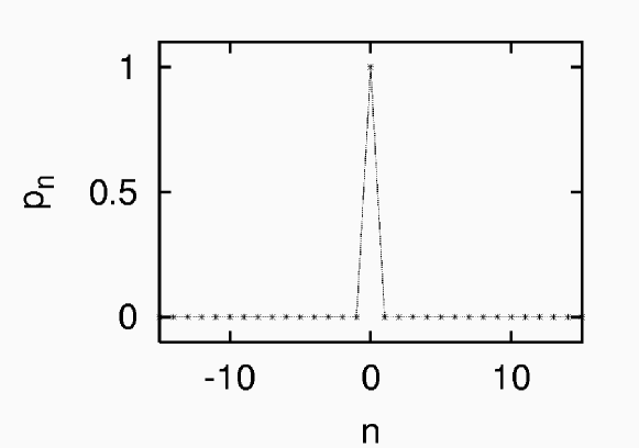
Figure 1: Occupation probabilities $p_{n}$ for a defect state in a one-dimensional lattice (1) with a defect of the form (4) at the site $n=0$; the defect strength is $\nu/W=0.1$. The upper figure shows the state in the absence of periodic forcing; it is exponentially localized according to Eq. (8). The lower figure shows the defect Floquet state when the system is driven with frequency $\hbar\omega/W=7.5$ and amplitude $eFd/(\hbar\omega)=2.4048$, corresponding to the first zero of ${\rm J}_{0}$. Since the effective band width (15) is zero here, the defect state is localized almost entirely at the defect site.

IV Energy splitting and quasienergy splitting for communicating defects

In the following, the real amplitudes $a_{\ell}$ for the state bound by a single defect placed at a site $\gamma>0$ are normalized such that

$$\sum_{\ell=1}^{\infty}\left|a_{\ell}\right|^{2}=1\;,$$ (16)

which implies that the normalization constant ${\cal N}$ in Eq. (10) is now given by

$${\cal N} = \left({{\sum_{i=1}^{\gamma}x_{-}^{2(\gamma-i)}+\sum_{i=\gamma+1}^{\infty}x_{-}^{2(i-\gamma)}}}\right)^{-1/2}$$ (17)

$$= \sqrt{\frac{1-x_{-}^{2}}{1+x_{-}^{2}-x_{-}^{2\gamma}}}\;.$$

This defect state obeys the Schrödinger equation

$$\left(\hat{H}_{0}+\hat{V}_{\rm r}\right)\left|\psi_{0}\right>=E_{0}\left|\psi_{0}\right>\;.$$ (18)

Next, a second, identical defect is introduced into the left half of the lattice at the site labeled $-\gamma$, as described by

$$\hat{V}_{\rm l}={\left|-\gamma\right.\rangle}\nu{\langle\left.-\gamma\right|}\;,\quad\gamma>0\;.$$ (19)

The two defects then carry two localized states $\left|\psi_{1}\right>$ and $\left|\psi_{2}\right>$, obeying the eigenvalue equations

$$\left(\hat{H}_{0}+\hat{V}_{\rm r}+\hat{V}_{\rm l}\right)\left|\psi_{1}\right> = E_{1}\left|\psi_{1}\right>\;,$$ (20)

$$\left(\hat{H}_{0}+\hat{V}_{\rm r}+\hat{V}_{\rm l}\right)\left|\psi_{2}\right> = E_{2}\left|\psi_{2}\right>\;.$$ (21)

By symmetry, good approximations to these two defect states are given by the even and odd linear combinations

$$\left|\psi_{1,2}\right>=\sum_{\ell=-\infty}^{\infty}\frac{1}{\sqrt{2}}\left(a_{\ell}\pm a_{-\ell}\right)\left|\ell\right>\;.$$ (22)

From these, auxiliary wave functions

$$\widetilde{\left|{\psi}_{0}\right>} \equiv \sum_{\ell=1}^{\infty}a_{\ell}\left|\ell\right>$$ (23)

$$\mbox{and}\quad\widetilde{\left|{\psi}_{1}\right>} \equiv \sum_{\ell=1}^{\infty}\frac{1}{\sqrt{2}}\left(a_{\ell}+a_{-\ell}\right)\left|\ell\right>$$ (24)

are defined, which have nonvanishing amplitudes in the right half of the lattice only. Forming the scalar product of Eq. (18) with $\widetilde{\left<\psi_{1}\right|}$ then gives

$$\widetilde{\left<\psi_{1}\right|}\hat{H}_{0}+\hat{V}_{\rm r}\left|\psi_{0}\right>=E_{0}\widetilde{\left<\psi_{1}\right|}\left.\!\psi_{0}\right>\;;$$ (25)

forming that of Eq. (20) with $\widetilde{\left<\psi_{0}\right|}$ leads to

$$\widetilde{\left<\psi_{0}\right|}\hat{H}_{0}+\hat{V}_{\rm r}\left|\psi_{1}\right>=E_{1}\widetilde{\left<\psi_{0}\right|}\left.\!\psi_{1}\right>\;,$$ (26)

since $\widetilde{\left<\psi_{0}\right|}\hat{V}_{\rm l}=0$ (see Eqs. (19) and (23)). By definition, $\widetilde{\left<\psi_{1}\right|}\left.{\psi}_{0}\right>=\widetilde{\left<\psi_{0}\right|}\left.{\psi}_{1}\right>$. Hence, subtracting the above two equations yields

$$\left(E_{0}-E_{1}\right)\widetilde{\left<\psi_{1}\right|}\left.\!\psi_{0}\right>=\widetilde{\left<\psi_{1}\right|}\hat{H}_{0}\left|\psi_{0}\right>-\widetilde{\left<\psi_{0}\right|}\hat{H}_{0}\left|\psi_{1}\right>\;.$$ (27)

It is now stipulated that the localization of the state $\left|{\psi}_{0}\right>$ around the site $\gamma>0$ be sufficiently strong that its amplitudes in the left half of the lattice are negligible. One then has

$$\widetilde{\left<\psi_{1}\right|}\left.{\psi}_{0}\right>\simeq\frac{1}{\sqrt{2}}\widetilde{\left<\psi_{0}\right|}\left.{\psi}_{0}\right>=\frac{1}{\sqrt{2}}\;,$$ (28)

leading to

$$E_{0}-E_{1} \simeq -\frac{W}{4}\sum_{\ell=1}^{\infty}\Big{\{}\left(a_{\ell}\!+\!a_{-\ell}\right)a_{\ell+1}+\left(a_{\ell}\!+\!a_{-\ell}\right)a_{\ell-1}\Big{\}}$$ (29)

$$+\frac{W}{4}\sum_{\ell=1}^{\infty}\Big{\{}a_{\ell}\left(a_{\ell+1}\!+\!a_{-\ell-1}\right)$$

$$\qquad\qquad\qquad+a_{\ell}\left(a_{\ell-1}\!+\!a_{-\ell+1}\right)\Big{\}}$$

$$= -\frac{W}{4}\sum_{\ell=1}^{\infty}\Big{\{}\big{(}a_{-\ell}a_{\ell+1}-a_{-\ell+1}a_{\ell}\big{)}$$

$$\qquad\qquad+\big{(}a_{-\ell}a_{\ell-1}-a_{-\ell-1}a_{\ell}\big{)}\Big{\}}\;.$$

These telescope series can be summed immediately ($\sum_{n=1}^{N}\left(b_{n}-b_{n-1}\right)=b_{N}-b_{0}$ and $\lim_{\ell\rightarrow\infty}a_{\ell}=0$), resulting in

$$E_{0}-E_{1}=\frac{W}{4}\left(a_{1}-a_{-1}\right)a_{0}\;.$$ (30)

In the same manner, one also derives

$$E_{2}-E_{0}=\frac{W}{4}\left(a_{1}-a_{-1}\right)a_{0}\;.$$ (31)

Summing these two equations finally leads to a surprisingly simple expression for the splitting of the energies associated with the two defects:

$$E_{2}-E_{1}=\frac{W}{2}\left(a_{1}-a_{-1}\right)a_{0}\;.$$ (32)

Since $\left(a_{1}-a_{-1}\right)/2$ can be taken as the discrete derivative of the wave function at the site $\ell=0$, the energy splitting is determined by the product of the wave function itself and its derivative halfway between the two defects, i.e., by the current prevailing there. Thus, this Eq. (32) constitutes a discrete analog of Herring’s formula, which describes the tunneling splitting for wave functions in double well potentials LL ; Herring62 ; Gutzwiller90 . In view of Eqs. (10) and (17), one then has

$$\Delta E \equiv E_{2}-E_{1}$$ (33)

$$= p\frac{W}{2}\frac{1-x_{-}^{2}}{1+x_{-}^{2}-x_{-}^{2\gamma}}x_{-}^{2\gamma}\left(x_{-}-x_{-}^{-1}\right)\;,$$

or

$$\frac{\Delta E}{E_{0}}=-\frac{\left(1-x_{-}^{2}\right)^{2}x_{-}^{2\gamma-1}}{\left(1+x_{-}^{2}-x_{-}^{2\gamma}\right)\sqrt{\frac{4\nu^{2}}{W^{2}}+1}}\;.$$ (34)

As with a single defect, the energy eigenvalues are replaced by the corresponding quasienergies in the presence of time-periodic forcing, and the energy splitting turns into a quasienergy splitting. The above result (34), with $W$ replaced by $W_{\rm eff}$ according to Eq. (15), should also be a good approximation to the quasienergy splitting if the driving frequency is sufficiently high.

In order to check this hypothesis, the time-dependent Schrödinger equation for the periodically forced two-defect system has been solved numerically, and the quasienergies for the localized states have been obtained. The results for two defects at $\gamma=\pm 3$, with $\nu/W=0.1$ and $\hbar\omega/W=7.5$, are plotted in Fig. 2 as functions of the scaled amplitude $eFd/(\hbar\omega)$. As can be seen, the agreement between the analytical approximation and the exact numerical data becomes excellent when $eFd/(\hbar\omega)>1$.

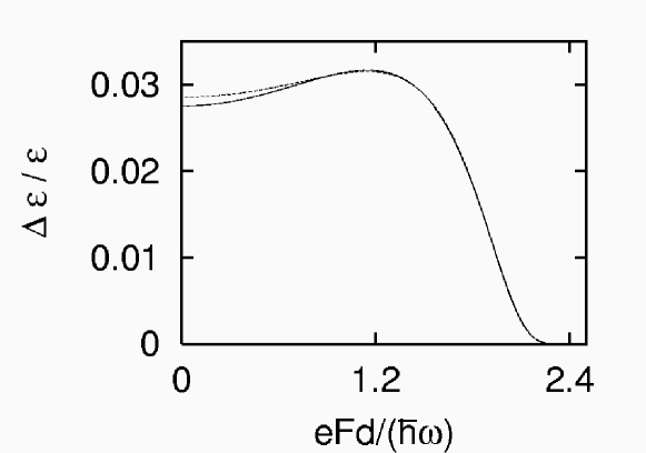
Figure 2: Relative splitting of the quasienergies in a periodically driven lattice with two identical defects of strength $\nu/W=0.1$ situated at $\gamma=\pm 3$, under the influence of forcing with frequency $\hbar\omega/W=7.5$. The full line shows the exact, numerically obtained data. The dashed line results from the Herring-type approximation (34), with the bandwidth $W$ replaced by the effective band width (15).

V Controlled population transfer

It is assumed now that initially, at time $t=0$, the particle is localized at one of the two defects, and the periodic force is present. Denoting the two Floquet functions associated with the defects at the given driving amplitude $F$ by $\left|u_{1,2}^{F}(t)\right>$, and their quasienergies by $\varepsilon^{F}_{1,2}$, the initial state is given by a superposition

$$\left|\psi(0)\right>=\frac{1}{\sqrt{2}}\big{(}\left|u_{1}^{F}(0)\right>\pm\left|u_{2}^{F}(0)\right>\big{)}\;.$$ (35)

Under the influence of forcing with constant amplitude, this state evolves in time according to

$$\left|\psi(t)\right> = \frac{1}{\sqrt{2}}\Big{(}\left|u_{1}^{F}(t)\right>\pm\left|u_{2}^{F}(t)\right>\exp(-{\rm i}\Delta\varepsilon^{F}t/\hbar)\Big{)}$$ (36)

$$\times\exp(-{\rm i}\varepsilon_{1}^{F}t/\hbar)\;,$$

where

$$\Delta\varepsilon^{F}=\varepsilon_{2}^{F}-\varepsilon_{1}^{F}$$ (37)

denotes the quasienergy splitting. Hence, the particle is coherently oscillating between the two defects; the transfer time $T_{\rm trans}$, after which the particle will be found at the other defect, is given by

$$T_{\rm trans}=\frac{\pi\hbar}{\Delta\varepsilon^{F}}$$ (38)

and thus depends on the driving amplitude $F$.

When the amplitude changes sufficiently slowly in time, the system responds in an adiabatic manner BreuerHolthaus89 . Hence, under the influence of a slowly varying amplitude $F(t)$, the initial state (35) follows the instantaneous Floquet states and evolves into

$$\left|\psi(t)\right> = \frac{1}{\sqrt{2}}\left[\left|u_{1}^{F(t)}(t)\right>\right.$$ (39)

$$\left.\pm\left|u_{2}^{F(t)}(t)\right>\exp\left(-\frac{{\rm i}}{\hbar}\int_{0}^{t}\!{\rm d}\tau\,\Delta\varepsilon^{F(\tau)}\right)\right]$$

$$\times\exp\left(-\frac{{\rm i}}{\hbar}\int_{0}^{t}\!{\rm d}\tau\,\varepsilon_{1}^{F(\tau)}\right)\;.$$

This implies that the transfer time from one defect to the other now is given by the relation

$$\frac{1}{\hbar}\int_{0}^{T_{\rm trans}}\!{\rm d}\tau\,\Delta\varepsilon^{F(\tau)}=\pi\;,$$ (40)

which constitutes an immediate analog of the $\pi$-pulse-condition known from two-level systems AllenEberly87 . This is the physics which will now be exploited for coherent control of population transfer between two communicating defects.

To this end, the driving amplitude $F(t)$ is shaped such that one has $eFd/(\hbar\omega)=j_{0,1}$ for $t\leq 0$, so that the defect Floquet states are confined to their respective sites, and the communication between the two defects is effectively disrupted. Then the amplitude is adiabatically lowered such that the defect states start to overlap significantly, and the particle initially tied to one defect oscillates to the other. If the amplitude then rises again and reaches the “collapse” value

$$F_{\rm collapse}=j_{0,1}\frac{\hbar\omega}{ed}$$ (41)

at $t=T_{\rm pulse}$, and is kept constant thereafter, the particle has been transferred to the final state, and will stay there. The time $T_{\rm pulse}$ is chosen such that

$$\frac{1}{\hbar}\int_{0}^{T_{\rm pulse}}\!{\rm d}\tau\,\Delta\varepsilon^{F(\tau)}=\varphi\;;$$ (42)

to obtain a transfer from one defect to the other, again $\varphi=\pi$ has to be chosen.

For a matter-of-principle demonstration of this scenario, one may employ the envelope function

$$F(t) = F_{\rm collapse}$$

$$\times \frac{\exp\left(-\frac{t^{2}}{2T_{\rm ramp}^{2}}\right)+a+\exp\left(-\frac{\left(t-T_{\rm pulse}\right)^{2}}{2T_{\rm ramp}^{2}}\right)}{a+1+\exp\left(-{\frac{T_{\rm pulse}^{2}}{2T_{\rm ramp}^{2}}}\right)}$$

for $0\leq t\leq T_{\rm pulse}$, where $T_{\rm ramp}$ quantifies the characteristic time interval during which the amplitude is ramped down and up again, with $T\ll T_{\rm ramp}\ll T_{\rm pulse}$ being understood. The parameter $a$ has been introduced in order to allow for a nonvanishing amplitude at intermediate times, at $t\approx T_{\rm pulse}/2$.

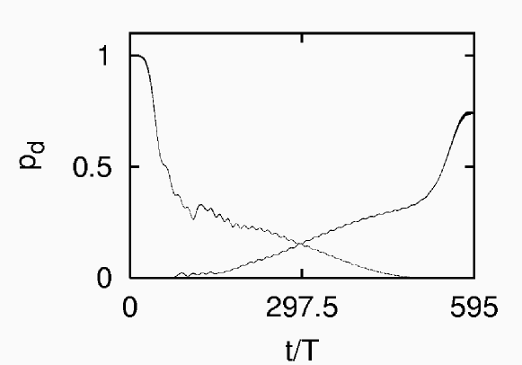
Figure 3: Incomplete population transfer resulting from fast, nonadiabatic changes of the amplitude function. There are two defects at $\gamma=\pm 3$ with strength $\nu/W=0.1$; the forcing frequency is $\hbar\omega/W=7.5$. The envelope function is given by Eq. (V), with $a=1.5$, $T_{\rm ramp}=50\,T$, and $T_{\rm pulse}=595\,T$. Plotted are the probabilities to find the particle at the two defect sites.

The above considerations rely heavily on the adiabatic principle; if the parameter variation proceeds too fast, complete population transfer is not achieved. This is illustrated in Fig. 3 for a system with defect parameters $\gamma=\pm 3$ and $\nu/W=0.1$, subjected to forcing with frequency $\hbar\omega/W=7.5$ and the envelope function (V), setting $a=1.5$, $T_{\rm ramp}=50\,T$, and $T_{\rm pulse}=595\,T$. Under these conditions, the transfer remains incomplete; slight oscillations visible in the occupation probabilities of the defect sites indicate non-adiabatic dynamics. However, Fig. 4 demonstrates that the desired result is obtained when the time scales are prolonged: With $T_{\rm ramp}=200\,T$ and $T_{\rm pulse}=1070\,T$, one has practically complete transfer.

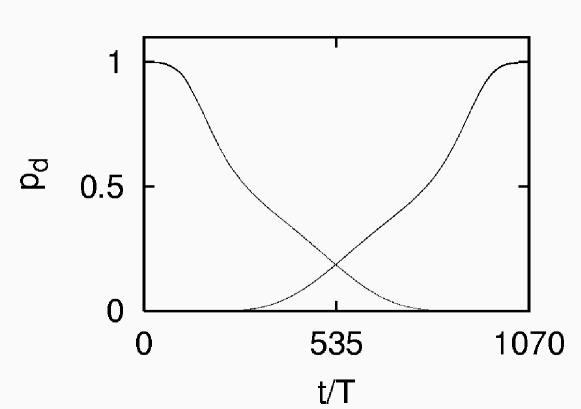
Figure 4: Adiabatic population transfer at communicating defects: Now $T_{\rm ramp}=200\,T$, and $T_{\rm pulse}=1070\,T$; the other parameters are as in Fig. 3.

It is, of course, also possible to employ the method outlined here to prepare the particle in superpositions of defect states. For instance, if one chooses $T_{\rm pulse}$ such that the phase integral in Eq. (40) yields $\pi/2$, rather than $\pi$, the resulting state describes a particle which, after initially being localized at a single defect, is eventually found with equal probability on either one. In the same manner, any desired probability ratio can be obtained; Fig. 5 shows an example where the particle remains with a probability of $1/4$ at the initial defect, and is found with a probability of $3/4$ at the other one, after forcing according to Eq. (V).

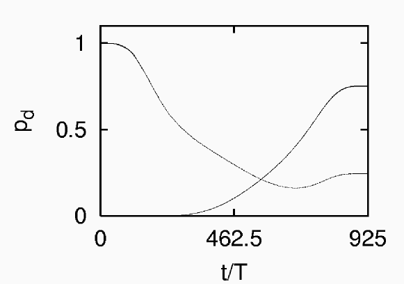
Figure 5: Probabilities to find the particle at the two defects for $T_{\rm ramp}=200\,T$ and $T_{\rm pulse}=925\,T$; the other parameters are as in Fig. 3. This choice of parameters aims at producing a coherent, Schrödinger cat-like state, with probabilities of $25\%$ and $75\%$ for finding the particle at the defects. Arbitrary other final probability ratios can be achieved as well.

VI Conclusion

It has been shown in this paper that a periodic force can drastically alter the energy splitting associated with the two states bound by two identical defects in a one-dimensional tight-binding lattice. In the presence of the force, the band width $W$ entering the energy splitting (34) has to be replaced by the effective width (15), so that the splitting can be monitored within wide ranges, and even be completely suppressed. Thus, the times required for coherent population exchange between the defects can be varied over several orders of magnitude by adjusting the amplitude of the force.

The strategy employed here to give a matter-of-principle illustration of coherent control of population transfer relies on the adiabatic principle, and thus is restricted to forces with slowly varying amplitudes. It appears possible to overcome this restriction: Utilizing techniques developed for the coherent control of molecules JudsonRabitz92 ; AssionEtAl98 , it might be possible to design even rapidly changing envelopes which effectuate a guided transport of a particle from one defect to the other, or to create superposition states with well-defined weights. This might open up new perspectives for the design of quantum logical devices.

Appendix A Eigenfunction for a single defect

In order to demonstrate that ${\left|\psi_{0}\right.\rangle}$ as defined by Eqs. (9) and (10) indeed is an eigenfunction of the single-defect Hamiltonian (5) with the energy eigenvalue (6), it is helpful to invoke the definition (7), and to write $\nu=W\frac{\nu}{W}=Wp\left|\frac{\nu}{W}\right|$. One then obtains

$$\hat{H}{\left|\psi_{0}\right.\rangle}= {\left|\gamma\right.\rangle}pW\left|\frac{\nu}{W}\right|{\langle\left.\gamma\right|}{\psi_{0}}\rangle$$

$$- \frac{W}{4}\sum_{\ell=-\infty}^{\infty}\left\{{\left|\ell\right.\rangle}{\langle\left.\ell+1\right|}+{\left|\ell\right.\rangle}{\langle\left.\ell-1\right|}\right\}{\left|\psi_{0}\right.\rangle}$$

$$= pW\left|\frac{\nu}{W}\right|a_{\gamma}{\left|\gamma\right.\rangle}-\frac{W}{4}\sum_{\ell=-\infty}^{\infty}\left(a_{\ell-1}+a_{\ell+1}\right){\left|\ell\right.\rangle}\;.$$

Singling out the defect site, one has

$$\hat{H}{\left|\psi_{0}\right.\rangle}= \left(pW\left|\frac{\nu}{W}\right|a_{\gamma}-\frac{W}{4}\left(a_{\gamma-1}+a_{\gamma+1}\right)\right){\left|\gamma\right.\rangle}$$ (45)

$$- \frac{W}{4}\sum_{\genfrac{}{}{0.0pt}{1}{\ell=-\infty}{\ell\neq\gamma}}^{\infty}\left(a_{\ell-1}+a_{\ell+1}\right){\left|\ell\right.\rangle}\;.$$

Utilizing the explicit expression (10) for the amplitudes $a_{\ell}$, this leads to

$$\hat{H}{\left|\psi_{0}\right.\rangle}= \left(pW\left|\frac{\nu}{W}\right|+p\frac{W}{2}x_{-}\right)a_{\gamma}{\left|\gamma\right.\rangle}$$

$$- \frac{W}{4}\sum_{\genfrac{}{}{0.0pt}{1}{\ell=-\infty}{\ell\neq\gamma}}^{\infty}(-p)(x_{-}^{-1}+x_{-})a_{\ell}{\left|\ell\right.\rangle}$$

$$= p\frac{W}{2}\sqrt{\frac{4\nu^{2}}{W^{2}}+1}\,a_{\gamma}{\left|\gamma\right.\rangle}$$ (46)

$$+ p\frac{W}{4}\sum_{\genfrac{}{}{0.0pt}{1}{\ell=-\infty}{\ell\neq\gamma}}^{\infty}(x_{-}^{-1}+x_{-})a_{\ell}{\left|\ell\right.\rangle}\;.$$

According to the definition (11), one has $x_{-}^{-1}=x_{+}$. Hence, $x_{-}^{-1}+x_{-}=x_{+}+x_{-}=2\sqrt{\frac{4\nu^{2}}{W^{2}}+1}$, which implies

$$\hat{H}{\left|\psi_{0}\right.\rangle}=p\frac{W}{2}\sqrt{\frac{4\nu^{2}}{W^{2}}+1}\sum_{\ell=-\infty}^{\infty}a_{\ell}{\left|\ell\right.\rangle}\;.$$ (47)

This proves the assertion.

References

• (1) M. Wagner and W. Zwerger, Phys. Rev. B 55, R10217 (1997).
• (2) M. Grifoni and P. Hänggi, Phys. Rep. 304, 229 (1998).
• (3) W. Li and L. E. Reichl, Phys. Rev. B 62, 8269 (2000).
• (4) D. F. Martinez, L. E. Reichl, and G. A. Luna-Acosta, Phys. Rev. B 66, 174306 (2002).
• (5) D. W. Hone and M. Holthaus, Phys. Rev. B 48, 15123 (1993).
• (6) J. H. Shirley, Phys. Rev. 138, B979 (1965).
• (7) Ya. B. Zel’dovich, Zh. Eksp. Theor. Fiz. 51, 1492 (1966) [Sov. Phys. JETP 24, 1006 (1967)].
• (8) V.I. Ritus, Zh. Eksp. Theor. Fiz. 51, 1544 (1966) [Sov. Phys. JETP 24, 1041 (1967)].
• (9) M. Holthaus, Phys. Rev. Lett. 69, 351 (1992).
• (10) M. Holthaus and D.W. Hone, Phys. Rev. B 47, 6499 (1993).
• (11) D. H. Dunlap and V. M. Kenkre, Phys. Rev. B 34, 3625 (1986).
• (12) T. Meier, G. von Plessen, P. Thomas, and S. W. Koch, Phys. Rev. B 51, 14490 (1995).
• (13) L. D. Landau and E. M. Lifshitz, Quantum Mechanics (Butterworth-Heinemann, Oxford, 1997), § 50.
• (14) C. Herring, Rev. Mod. Phys. 34, 631 (1962).
• (15) M. C. Gutzwiller, Chaos in Classical and Quantum Mechanics (Springer, New York, 1990), § 14.6.
• (16) H. P. Breuer and M. Holthaus, Z. Phys. D 11, 1 (1989).
• (17) L. Allen and J. H. Eberly, Optical Resonance and Two-Level Atoms, (Dover Publications, New York, 1987)
• (18) R. S. Judson and H. Rabitz, Phys. Rev. Lett. 68, 1500 (1992).
• (19) A. Assion, T. Baumert, M. Bergt, T. Brixner, B. Kiefer, V. Seyfried, M. Strehle, and G. Gerber, Science 282, 919 (1998).