Diffusion-limited aggregation with jumps and flights

Abstract

The paper suggests a generalisation of the diffusion-limited aggregation (DLA) based on using a general stochastic process to control particle movements before sticking to a growing cluster. This leads to models with variable characteristics that can provide a single framework for treating a number of earlier models of fractal growth: the DLA, the Eden model and the ballistic aggregation. Additionally, a classification of fractal growth models is suggested.

1 Introduction

Stochastic models of fractal growth have inspired a number of studies and applications in applied sciences. The best known models are the diffusion-limited aggregation (DLA), the Eden model, and the ballistic aggregation. These basic models operate according the the following basic rule.

The initial starting point for the growing cluster is fixed, so that the primary cluster consists of a single particle (or pixel for simulations on discretised computer screen). At every step another pixel (particle) is attached to the cluster according to some rule so that the cluster remains connected with respect to some neighbouring relationship. This is repeated on every new step until the cluster reaches the predetermined size.

The details depend on the model. Note that a number of growth models are discussed in [10, 12], where further references, simulated and real pictures and discussions can be found.

The Eden model.

This is a lattice model which was originally suggested as a model for growth of cell colonies (like tumours). At any time moment, all neighbours of the active cluster form the growth zone; a new point to be attached to the cluster is picked from all these neighbours, where all neighbours have equal chances to be chosen. Some modifications of the Eden model are discussed in [6].

DLA.

This famous model for fractal growth called diffusion-limited aggregation (DLA) goes back to pioneering papers by Witten and Sander [13, 14]. In this model, every new particle moves according to Brownian motion starting at infinity (or just far enough from the growing cluster). When the particle touches the cluster, it sticks to it irreversibly. This model is called off-lattice DLA in contrast to lattice DLA where each particle is represented by a pixel on the grid and moves according to the symmetric random walk on the grid until it reaches one of the pixels adjacent to the cluster and then sticks to the cluster. This produces finger-like structure of fractal type.

The model can be rephrased according to the description of the Eden model, but where neighbours are not equally likely to be attached to the cluster. Instead, the next pixel is chosen among all neighbours with a distribution proportional to the equilibrium electrostatic potential on the boundary of the existing cluster, which is the solution of $\Delta u=0$ where $\Delta=\nabla^{2}$ is the Laplace operator. Therefore, DLA captures the essential features of a typical dynamic growth process that is related to the Laplace equation.

Ballistic aggregation.

In this model new particles move along straight lines (ballistic trajectories) until they hit the cluster or disappear (leave the window of observation). If the mobile (flying) particle contacts the growing cluster, it sticks at the point of the first touch.

The aim of the current paper.

This paper suggests a generalisation of the DLA model which encompasses a number of known models, including the Eden model, the standard DLA and the ballistic aggregation. The basic idea is to replace the Brownian motion in the definition of the standard DLA with a general stochastic process, possibly having jumps and long-range dependence. By varying the characteristics of the stochastic process it is possible to amalgamate DLA, the Eden model and ballistic aggregation into a single stochastic growth model. In particular, it will be shown that the introduced model provides a reasonable tradeoff between the DLA, ballistic and Eden models and has realisations which share particular features of the above mentioned models.

We will report several simulation results in two dimensions for lattice models and moderate numbers of particles in the cluster. Following the same ideas it is possible to extend simulations to off-lattice models and increase the size of the cluster by appealing to efficient algorithms for DLA simulations known from the literature, see [7]. Finally, we suggest a classification of growth models, which might be useful in future to unify a number of specific models known in the literature.

2 Markov-limited aggregation

The classical DLA model assumes that every new particle moves according to Brownian motion (or a simple random walk in the lattice model) starting from infinity (or just sufficiently far from the cluster).

Brownian motion is just a particular example of a stochastic process that can be used to induce the particles’ movements. Natural generalisations arise from using other stochastic processes in place of Brownian motion. Biased growth was considered in [4]. In this case a particle performs a biased random walk where the bias is determined by the particle’s position, so that the corresponding stochastic processes is not spatially homogeneous. This leads to DLA-like patterns but with varying fractal dimension depending on the introduced bias. Growth in non-Laplacian fields which appears in the presence of electrostatic field in addition to the diffusion component was studied in [8]. This is related to the inhomogeneous DLA model considered in [9].

Let us assume that particles move according to a Markov process $\xi_{t}$, $t\geq 0$, with values in the $d$-dimensional space ${\mathbf{R}}^{d}$ The Markov process is described by its transition kernel $P(t,x,s,A)$, which can be identified as the probability that $\xi_{s}\in A$ given that $\xi_{t}=x$. Loosely speaking, $P(t,x,s,A)$ is the probability of moving from the state $x$ at time $t$ to the set $A$ at time $s$. Assume that the process is (time) homogeneous so that $P(t,x,s,A)$ depends on $s-t$ rather than $t$ and $s$ separately. Then the transition kernel is written as $P_{h}(x,A)=P(t,x,t+h,A)$.

A Markov process generates two families of operators. One family acts on bounded functions $f$ as

$$(T_{t}f)(x)=\int P_{t}(x,dy)f(y)\,,\quad t\geq 0,\;x\in{\mathbf{R}}^{d}\,.$$

Note that $(T_{t}f)(x)$ can be interpreted as the expected value of $f(\xi_{t})$ given that $\xi_{0}=x$. The other family of operators acts on signed measures $\mu$ with finite total variation (the variation equals the sum of the absolute values of the positive and negative components of $\mu$) as

$$(T^{*}_{t}\mu)(B)=\int P_{t}(x,B)\mu(dx)\,,\quad t\geq 0\,,$$ (1)

where $B$ is a measurable subset of ${\mathbf{R}}^{d}$. The operators acting on measures by (1) are more important in the sequel, since $(T^{*}_{t}\mu)$ can be interpreted as the distribution of the mass (or charge if $\mu$ is a signed measure) at time $t$ if the initial distribution is given by $\mu$ and all elementary masses (or charges) are being moved along the trajectories of $\xi_{t}$.

For properties of the Markov process, the behaviour of $T_{t}$ and $T^{*}_{t}$ as $t\downarrow 0$ is crucial. This behaviour is described by two generating operators which appear as “derivatives” of $T_{t}$ and $T^{*}_{t}$ at $t=0$ and are defined as follows

$$(Af)(x) =\lim_{t\downarrow 0}t^{-1}((T_{t}f)(x)-f(x))\,,$$ (2)

$$(A^{*}\mu)(B) =\lim_{t\downarrow 0}t^{-1}((T^{*}_{t}\mu)(B)-\mu(B))\,,$$ (3)

provided that the corresponding limits exist. The operators $A$ and $A^{*}$ are adjoint, i.e.

$$\langle Af,\mu\rangle=\int(Af)(x)\mu(dx)=\int f(x)(A^{*}\mu)(dx)=\langle f,A^{*}\mu\rangle$$

for all $f$ and $\mu$ from the domains of existence of the corresponding operators.

It is well known that if $\xi_{t}$ is the Wiener process (or standard Brownian motion), then

$$(Af)(x)=\frac{1}{2}(\nabla^{2}f)(x)$$

for twice differentiable $f$ with bounded partial derivatives of the first and the second order. Here $\nabla^{2}=\Delta$ is the Laplace operator, so that

$$(\nabla^{2}f)(x)=\sum_{i=1}^{d}\frac{\partial^{2}f}{\partial x_{i}^{2}}(x)\,.$$

If a signed measure $\mu$ has a sufficiently smooth density $u$, then

$$(A^{*}\mu)(dx)=\frac{1}{2}(\nabla^{2}u)(x)dx\,.$$

This fact is widely used in the theory of DLA to relate the properties of the growing DLA cluster to the Laplace equation.

Now define a growth process that is controlled by a general Markov process $\xi_{t}$ instead of the Wiener process used to define the standard DLA. The growth starts with a ball of a small radius $r$ centred at the origin. Let $C$ be the current cluster. At every step a particle starts at the infinity, which in practice reduces to a random point $a$ uniformly distributed over the boundary of a sufficiently large sphere $S$ centred at the origin. The particle moves along the path of the Markov process $\xi_{t}$ (starting at $a$) until it either leaves $S$ or reaches the set $C^{r}=\{x:\;\rho(x,C)\leq r\}$ (which is the set of all points at distance no more than $r$ from $C$). In the first case the particle is killed as soon it leaves $S$, in the second case, a ball of radius $B_{r}(x)$ is attached to the cluster, where $x=\xi_{\tau}$ is the position of the particle when it first reaches $C^{r}$, so that $\tau=\inf\{t\geq 0:\;\xi_{t}\in C^{r}\}$.

The above description defines an off-lattice aggregation model determined by the law of the Markov process $\xi_{t}$. It allows a clear interpretation in terms of operators associated with the Markov process (the corresponding explanations for the standard DLA controlled by the Wiener process can be found in [2, Section 18.1]).

Let $\mu_{t}$ denote the distribution of particles at time $t$. Assume that $\mu_{t}$ has a density $u(x,t)$, so that $\mu_{t}(dx)=u(x,t)dx$. Every particle moves according to the Markov process, so that the density of particles at point $y$ and time $t+h$ is given by

$$(T^{*}_{h}\mu_{t})(dy)=\mu_{t+h}(dy)=\int P_{h}(x,dy)\mu_{t}(dx)\,.$$ (4)

Differentiation (4) with respect to $h$ and comparison with (3) lead to

$$A^{*}\mu_{t}=\frac{d}{dt}\mu_{t}\,.$$

In terms of the density $u(x,t)$ the above equation can be written as

$$\frac{\partial u}{\partial t}(x,t)=A^{*}u(x,t)\,.$$ (5)

For example, if $\xi_{t}$ is the standard Brownian motion, then (5) becomes

$$\frac{\partial u}{\partial t}(x,t)=\frac{1}{2}\nabla^{2}u(x,t)\,,$$

which is the diffusion equation or heat equation.

If the growth occurs very far from the place where new particles start their movement, $u(x)=u(x,t)$ can be considered as independent of $t$, so that (5) turns into

$$A^{*}u(x)=0$$ (6)

(which becomes $\nabla^{2}u=0$ for standard DLA). The boundary condition is $u=0$ at the boundary of the growing cluster and $u=u_{0}$ for $\|x\|=R$, where $R$ is the radius of the circle where new particles are being launched. Solving (6) allows us to find $u$ and then obtain the rate of growth at any point on the cluster’s boundary by computing the derivative of $u$ in the direction of the normal. Although the direct simulation of the growth process is easier than numerical solution of (6) for the growing cluster, equation (6) provides a useful theoretical interpretation and justification for the particular choice of the Markov process $\xi_{t}$, so that this choice is largely determined by equations that control the physics of the growth process.

3 Examples and simulations

The general setup.

In simulations on the discrete grid Markov processes are approximated by their discrete analogues. For example, the Wiener process becomes a nearest-neighbour symmetrical random walk, and a general process with independent increments corresponds to a random walk with varying step length and a possible linear drift. Every new particle starts on the boundary of a large circle and moves until it either leaves the circle or becomes a neighbour of the cluster.

When doing simulations on the discrete grid, it is quite typical to use noise reduction. The essence of noise reduction is that newly arrived particles are not immediately attached to the growing cluster. Instead, they are being accumulated so that a new site is attached to the cluster only when at least $n$ particles have been accumulated there. If $n=1$, then no noise reduction is present. In the simulations below we systematically work on the planar square grid and use the noise reduction parameter $n=4$ (which ensures a moderate noise reduction while computation time is increased by a factor of 4 only). The neighbouring relation on the planar square grid is chosen in such a way that a point (pixel) has 4 neighbours, each sharing one edge with this pixel. All simulations below present clusters of size $52,000$ (unless stated otherwise) simulated on the grid of size $1024\times 1024$ pixels.

The Wiener process and standard DLA.

Figure 1(a) shows a simulated cluster of 32,000 pixels generated with $\xi_{t}$ taken to be standard Brownian motion (or the Wiener process). The corresponding generating operator is the Laplace operator $A=(1/2)\nabla^{2}$, so that the growth corresponds to the models described by Laplace equation.

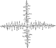
(a) The standard DLA (32,000 points)

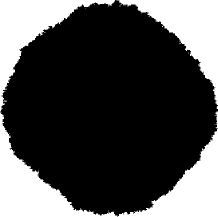
(b) The Eden model

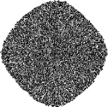
(c) The circular ballistic model

Figure 1: The standard DLA, the Eden model and the centre-bound ballistic aggregation.

White noise and the Eden model.

Assume that $\xi_{t}$ is a process with independent values (or white noise). At each step the particle moves to a site chosen completely random from all points in a disk of a sufficiently large radius. Figure 1(b) provides a simulated cluster. It is easy to see that the model so defined is exactly the Eden model. Indeed all pixels from the growth zone (adjacent to the existing cluster) have equal probabilities to be chosen, while all other pixels are discarded and do not influence the evolution. Clearly, from the point of view of simulations it is more efficient to use a standard way to simulate the Eden model, in comparison with the white noise simulation where many points are discarded. For the white noise case, operators $T_{t}$ and $T^{*}_{t}$ become identical and independent of $t$, so that the generating operators are trivial and equation (6) becomes the identity.

Diffusion processes.

Now assume that $\xi_{t}$ is a diffusion process. In this case, the generating operator $A$ is given by a general elliptic operator, so that (6) becomes

$$\frac{1}{2}\sum_{i,j=1}^{d}b_{ij}(x)\frac{\partial^{2}u}{\partial x_{i}\partial x_{j}}-\sum_{i=1}^{d}a_{i}(x)\frac{\partial u}{\partial x_{i}}=0\,,$$

where $x=(x_{1},\dots,x_{d})$, see, e.g., [3]. The matrix $(b_{ij}(x))_{ij}$ is called the diffusion matrix while $(a_{i}(x))_{i}$ is a transfer (drift) vector. In the spatially homogeneous case $b_{ij}(x)=b_{ij}$ and $a_{i}(x)=a_{i}$ do not depend on $x$.

Note that since diffusion processes are continuous, in the resulting cluster all points have been visited equally often, which means that new particles may not end up inside a cluster. This will not be the case for processes with jumps described below.

Processes with independent increments.

A stochastic process $\xi_{t}$ is said to have independent increments if $\xi_{s_{1}}-\xi_{s}$ and $\xi_{t_{1}}-\xi_{t}$ are independent for any $t\leq t_{1}\leq s\leq s_{1}$, so that increments of the process over disjoint intervals are independent. We assume that the process $\xi_{t}$ is homogeneous, so that the distribution of $\xi_{t+h}-\xi_{t}$ does not depend on $t$. The distribution of a homogeneous process with independent increments is determined by a transfer vector $(a_{i})_{i}$, a diffusion matrix $(b_{ij})_{ij}$ and a spectral measure $\Pi$, which is related to the distribution of jump lengths and the frequencies of jumps. The generating operator of the process is known for all stochastically continuous processes with independent increments, see [3, p. 344]. This covers processes with jumps and also with processes having an infinite number of (small) jumps in any finite time interval. We exclude this latter case and assume that the spectral measure $\Pi$ is finite. In this case the generating operator is given by

$$(Af)(x)=\sum_{i=1}^{d}a_{i}\frac{\partial f}{\partial x_{i}}+\frac{1}{2}\sum_{i,j=1}^{d}b_{ij}\frac{\partial^{2}f}{\partial x_{i}\partial x_{j}}+\int_{{\mathbf{R}}^{d}}(f(y+x)-f(x))\Pi(dy)$$ (7)

and is defined for all bounded twice continuously differentiable functions $f$ with bounded derivatives of first and second orders. In the discrete setup $\Pi(dy)=p_{\mathrm{j}}F(dy)$, where $p_{\mathrm{j}}$ is the probability of a jump at any given step and $F(\cdot)$ is the distribution of the jump’s length.

By taking an adjoint operator to $A$ defined in (7) we get, in place of (6),

$$-\sum_{i=1}^{d}a_{i}\frac{\partial u}{\partial x_{i}}+\frac{1}{2}\sum_{i,j=1}^{d}b_{ij}\frac{\partial^{2}u}{\partial x_{i}\partial x_{j}}+\int_{{\mathbf{R}}^{d}}(u(x-y)-u(x))\Pi(dy)=0\,.$$ (8)

It is anticipated that the above integro-differential equation can be used to model physical processes, where the integral term appears naturally alongside with the Laplacian or an elliptic operator.

For example, if there is no linear drift and the diffusion matrix is the unit matrix, then (8) turns into

$$(1-p_{\mathrm{j}})\frac{1}{2}\nabla^{2}u+p_{\mathrm{j}}{\mathbf{E}}(u(x-\eta)-u(x))=0\,,$$ (9)

where $\eta$ is a random vector which describes the jump and ${\mathbf{E}}$ denotes expectation. Assume that $\eta$ is an isotropic random vector, so that its distribution is determined by its length $J=\|\eta\|$. If $J\sim{\mathsf{Un}}(0,c)$ ($J$ is uniformly distributed over $[0,c]$), then in the planar case

$${\mathbf{E}}(u(x-\eta)-u(x))=(2\pi c)^{-1}\int_{B_{c}(0)}\|y\|^{-1}u(x-y)dy-u(x)\,,$$

where the integral is taken over the disk of radius $c$ centred at the origin. If $p_{\mathrm{j}}=1$, then the model has no diffusion component and (9) becomes

$${\mathbf{E}}u(x-\eta)=u(x)\,.$$ (10)

If $J=c$ is a constant, then (10) turns into

$$\frac{1}{2\pi c}\int_{\|y\|=c}u(x-y)dy=u(x)\,,$$ (11)

so that the value of $u$ at any point is equal to the mean value of the function on the circle of radius $c$ centred at this point. Note that in contrast to the definition of a general harmonic function, (11) is not required for all $c>0$ but just for a fixed value of $c$.

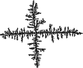
(a) $p_{\mathrm{j}}=0.3$, $J\sim{\mathsf{Un}}(0,10)$

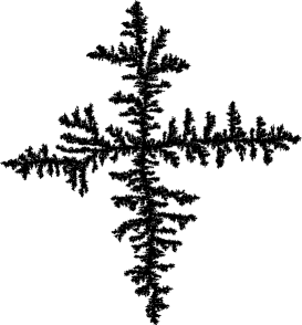
(b) $p_{\mathrm{j}}=0.7$, $J\sim{\mathsf{Un}}(0,10)$

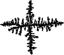
(c) $p_{\mathrm{j}}=1.0$, $J\sim{\mathsf{Un}}(0,10)$

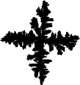
(d) $p_{\mathrm{j}}=0.5$, $J\sim{\mathsf{Un}}(0,20)$

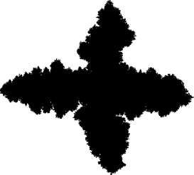
(e) $p_{\mathrm{j}}=0.5$, $J\sim{\mathsf{Un}}(0,40)$

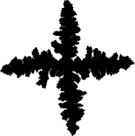
(f) $p_{\mathrm{j}}=1.0$, $J\sim{\mathsf{Un}}(0,20)$

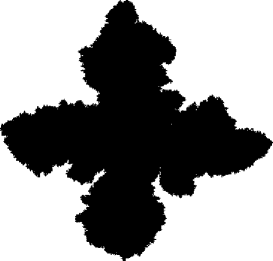
(g) $p_{\mathrm{j}}=1.0$, $J\sim{\mathsf{Un}}(0,40)$

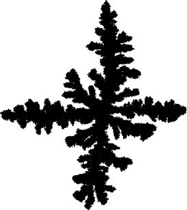
(h) $p_{\mathrm{j}}=1.0$, $J=10$

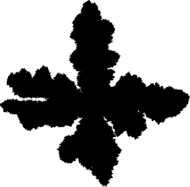
(i) $p_{\mathrm{j}}=1.0$, $J=20$

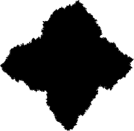
(j) $p_{\mathrm{j}}=0.5$, $J\sim{\mathsf{Un}}(0,80)$

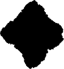
(k) $p_{\mathrm{j}}=1.0$, $J\sim{\mathsf{Un}}(0,80)$

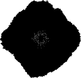
(l) $p_{\mathrm{j}}=1.0$, $J\sim{\mathsf{Un}}(0,160)$

Figure 2: Clusters obtained for Markov processes with jumps.

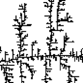
Fig1a

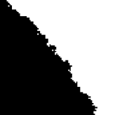
Fig1b

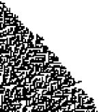
Fig1c

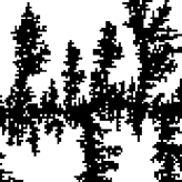
Fig2a

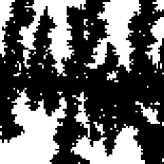
Fig2c

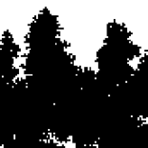
Fig2d

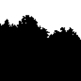
Fig2e

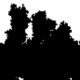
Fig2f

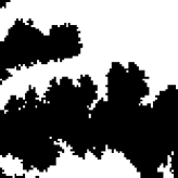
Fig2h

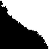
Fig2k

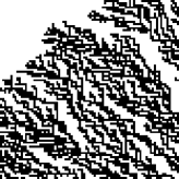
Fig3a

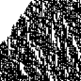
Fig3b

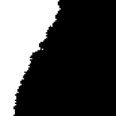
Fig3c

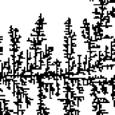
Fig4a

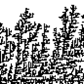
Fig4c

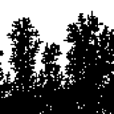
Fig4e

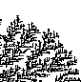
Fig4f

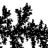
Fig4i

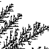
Fig5a

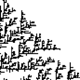
Fig5c

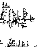
Fig5d

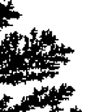
Fig5g

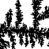
Fig6b

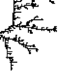
Fig6c

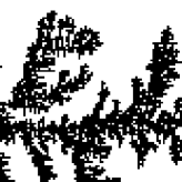
Fig6d

Figure 7: Enlargements of several clusters from previous figures (with the relevant references).

Figure 2 shows a number of simulated patterns obtained for the model which combines the Brownian motion component with jumps. It is easy to observe that the presence of jumps makes the patterns thicker while still retaining the fine structure of their boundaries (see enlargements in Figure 7). Larger jumps make clusters more compact, so that in the extreme case we can grow patterns which are similar to those from the Eden model.

The similar thickening effect is achieved within standard DLA by allowing particles to continue travelling after they become neighbours of the cluster for the first time, so that the particle can either stick to the cluster with some probability $p$ or continue travelling with probability $1-p$, see [14]. Then the particles can penetrate the cluster yielding thickening effect. However, the current setup naturally establishes relationships of this effect to some integro-differential equations.

Note that $J\sim{\mathsf{Un}}(0,c)$ results in a thicker cluster than $J=c/2$ (i.e. with $J$ being the expected value of the former). It should be noted that this thickening effect is entirely different from the effect that would be achieved if we enlarge the standard DLA model by a ball of some radius. The latter results in smoothing out the boundaries, while the clusters shown in Figure 2 have rough boundaries, as is clear from Figure 7.

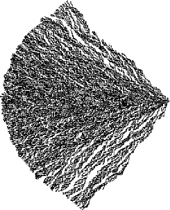
(a) $J=1$ (size 52,400)

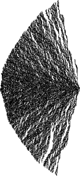
(b) $J=2$

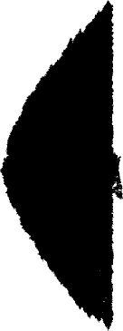
(c) $J=20$

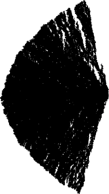
(d) $J\sim{\mathsf{Un}}(0,10)$

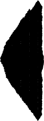
(e) $J=50$

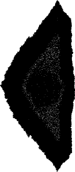
(f) $J=100$

Figure 3: Clusters obtained for the Markov model with $p_{\mathrm{j}}=1$ and jumps of fixed direction (horizontal to the right). The length of jumps $J$ is specified in every particular case. The size of clusters is 104,800 pixels unless specified otherwise.

Figure 3 shows clusters obtained for pure jump processes with jumps of a fixed direction. Assume that the jump $\eta$ has only a non-negative $x$ component, so that $\eta=(J,0)$ with $J>0$. All particles start from points uniformly distributed near the left border of the window and move to the right until they leave the window or stick to the cluster. It is not possible to let all particles start exactly on the left-hand side of the window, since this may lead to unwanted periodicity effects which are not compliant with the fact that ideally the particles are coming from infinity. To simulate coming from infinity, all particles start at points uniformly distributed within a rectangle located along the left border of the window and having width equal to the maximum possible value of $J$.

In particular if $J=c$ is constant, then (10) turns into

$$u(x-\eta)=u(x)\,.$$

Extending $u$ from its value on the points where particles start, we see that all points that can be reached from the left by moving (jumping) particles are equally likely to be attached to the cluster. In particular, if $J=1$, then all neighbours to the cluster which are visible from the left can be attached to the cluster with equal probabilities. For larger $J$ inner pixels can also be attached within a distance of at most $J$ from the left border of the growing cluster. This leads to the growth similar to that of the Eden model, but with a clearly expressed directionality.

It is interesting to note that the presence of jumps means that new particles can end up inside the cluster with their final jump. As a result of these final jumps they can end up in one of the already occupied sites, increasing the concentration of particles deposited at this particular site but without changing the shape of the cluster. Therefore, the defined growth model with jumps also provides a function that shows the number of particles accumulated at particular sites.

4 A general model with flights and jumps

Non-Markov particle movement.

The stochastic process $\xi_{t}$ that determines particles’ movements can be rather general and not necessarily Markov. One example worth special consideration describes ballistic trajectories of particles. We say that $\xi_{t}=\beta(t-t_{0})+a$ determines a flight which starts at point $a$ at time $t_{0}$ and has a velocity vector $\beta$. The basic model considered in this section deals with a stochastic process that has several components: a diffusion component, pure jumps, and a ballistic (or flight) component. For simulations on the discrete grid, we fix $p_{\mathrm{j}}$, the probability of a jump, and $p_{\mathrm{b}}$, the probability of a flight. This means that at any time $\xi_{t}$ performs a nearest neighbour random walk (or diffusion) with probability $1-p_{\mathrm{j}}-p_{\mathrm{b}}$, otherwise it jumps at vector $\eta$ (which is usually isotropic and has length $J$) or flies with probability $p_{\mathrm{b}}$, with the flight direction determined by a unit vector $\beta$ along the straight line at distance $L$.

There are two basic options for the distribution of $\beta$ which will be explored later on. First, $\beta$ can be an isotropic random vector. In the second case, $\beta$ depends on the position of the particle when it starts flying and points to the centre of the window (or towards the initial point of the cluster). In the first case we will speak about isotropic flights and in the second case about centre-bound flights. Clearly, mixtures of these two cases are also possible, but we will not discuss them here.

Unfortunately the process with flights is not Markov and so the model does not allow direct interpretation in terms of the generating operators.

Circular ballistic model.

Figure 1c provides an example of a circular ballistic model. In this model every new particle starts from a point uniformly distributed on a large circle. This point moves straight towards the centre of the cluster until it hits the cluster. In this case $p_{\mathrm{b}}=1$, the distance $L$ is sufficiently large (at least as large as the radius of the circle) and the random vector $\beta$ is a deterministic vector which depends on the position of the particle when it starts flying and is always directed towards the centre of the circle (as in the centre-bound case).

DLA with flights.

Figure 4 shows several clusters obtained for mixtures of processes with independent increments and possible flights. The directions of the flights are isotropic for all simulations shown in Figure 4.

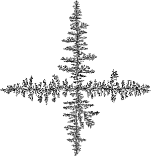
(a) $p_{\mathrm{j}}=0$, $p_{\mathrm{b}}=0.3$, $L=10$

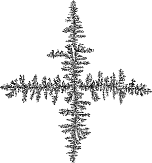
(b) $p_{\mathrm{j}}=0$, $p_{\mathrm{b}}=1.0$, $L=10$

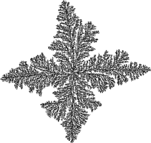
(c) $p_{\mathrm{j}}=0$, $p_{\mathrm{b}}=1.0$, $L=40$

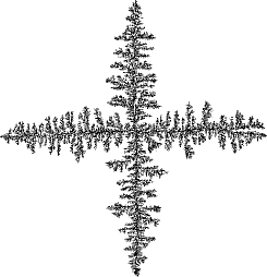
(d) $p_{\mathrm{j}}=0.3$, $J\sim{\mathsf{Un}}(0,10)$,
$p_{\mathrm{b}}=0.7$, $L=10$

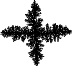
(e) $p_{\mathrm{j}}=0.3$, $J\sim{\mathsf{Un}}(0,40)$,
$p_{\mathrm{b}}=0.3$, $L=10$

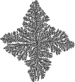
(f) $p_{\mathrm{j}}=0$, $p_{\mathrm{b}}=1.0$, $L=80$

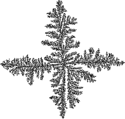
(g) $p_{\mathrm{j}}=0.3$, $J\sim{\mathsf{Un}}(0,10)$,
$p_{\mathrm{b}}=0.3$, $L=20$

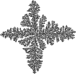
(h) $p_{\mathrm{j}}=0.3$, $J\sim{\mathsf{Un}}(0,10)$,
$p_{\mathrm{b}}=0.3$, $L=40$

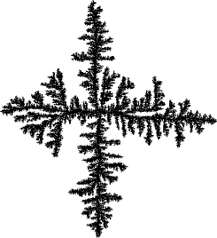
(i) $p_{\mathrm{j}}=0.5$, $J=10$,
$p_{\mathrm{b}}=0.5$, $L=5$

Figure 4: Ballistic aggregation with possible jumps and diffusion component.

It is easy to see that the increase in flight length $L$ results in models with fine structure (Figure 4c) still adhering to the typical structure of the standard DLA model. Jumps make patterns thicker in the same manner as they do for the model without flights.

Centre-bound flights.

A number of examples of DLA with centre-bound flights are shown in Figure 5. At every step with probability $p_{\mathrm{b}}$ the particle flies towards the origin a distance length $L$. Further simulations (not shown in Figure 5) show that if $L$ or $p_{\mathrm{b}}$ increase, then the realisations of the model look very similar to the circular ballistic model shown in Figure 1c.

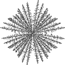
(a) $p_{\mathrm{j}}=0$, $p_{\mathrm{b}}=0.1$, $L=5$

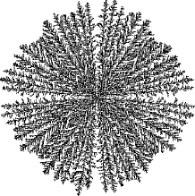
(b) $p_{\mathrm{j}}=0$, $p_{\mathrm{b}}=0.1$, $L=10$

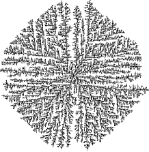
(c) $p_{\mathrm{j}}=0$, $p_{\mathrm{b}}=0.05$, $L=10$

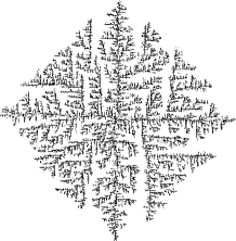
(d) $p_{\mathrm{j}}=0$, $p_{\mathrm{b}}=0.01$, $L=10$

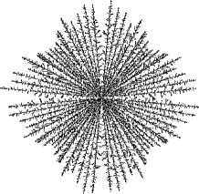
(e) $p_{\mathrm{j}}=0$, $p_{\mathrm{b}}=0.3$, $L=10$

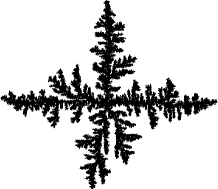
(f) $p_{\mathrm{j}}=0.99$, $J\sim{\mathsf{Un}}(0,10)$,
$p_{\mathrm{b}}=0.01$, $L=10$

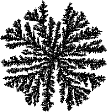
(g) $p_{\mathrm{j}}=0.9$, $J\sim{\mathsf{Un}}(0,10)$,
$p_{\mathrm{b}}=0.1$, $L=5$

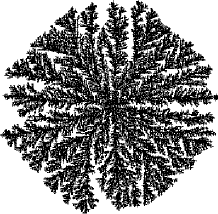
(h) $p_{\mathrm{j}}=0.9$, $J\sim{\mathsf{Un}}(0,10)$,
$p_{\mathrm{b}}=0.1$, $L=10$

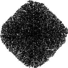
(i) $p_{\mathrm{j}}=0.9$, $J\sim{\mathsf{Un}}(0,80)$,
$p_{\mathrm{b}}=0.1$, $L=80$

Figure 5: Centre-bound ballistic aggregation with possible jumps and diffusion component.

Shooting models.

It is possible to define the following interesting variation of the DLA model with flights and jumps. Assume that all ballistic pieces of the trajectories are discarded if the particle does not hit the cluster while flying. In other words, if at any time the particle does not touch the cluster while flying, then it returns to the start of the flight and the last flight is discarded. This model can be naturally called the shooting model, assuming that a rifleman moves along a Markov process trying to shoot the cluster. If the rifleman hits the cluster with a shot then a new particle is attached to the cluster at the place of the first hit. If the rifleman does not hit the cluster, then he continues travelling, so that at any step he may attempt another shot with probability $p_{\mathrm{b}}$. Figure 6 shows several examples of the clusters obtained for the shooting model. Some of them have isotropic directions of shots (flights), while others have centre-bound shots (flights).

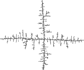
(a) $p_{\mathrm{j}}=0$, $p_{\mathrm{b}}=0.1$,
$L=10$ (isotropic),
cluster size 23,000

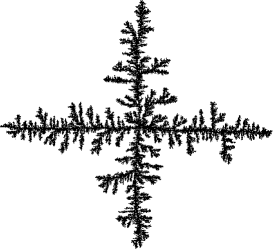
(b) $p_{\mathrm{j}}=0.9$, $J\sim{\mathsf{Un}}(0,10)$,
$p_{\mathrm{b}}=0.1$, $L=10$ (isotropic)

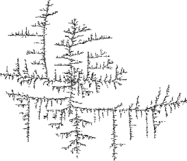
(c) $p_{\mathrm{j}}=0$, $p_{\mathrm{b}}=0.1$,
$L=10$ (centre-bound),
cluster size 34,000

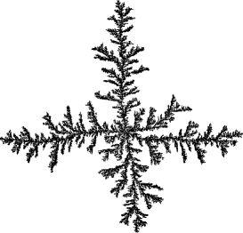
(d) $p_{\mathrm{j}}=0.9$, $J\sim{\mathsf{Un}}(0,10)$,
$p_{\mathrm{b}}=0.1$, $L=10$ (centre-bound)

Figure 6: The shooting model with isotropic flights (a),(b) and centre-bound flights (c),(d).

It is also possible to work out variations of the shooting model. For example, the jumps may also be discarded unless the final point of the jump is a neighbour to the cluster. This would correspond to a man throwing grenades and/or shooting from a gun.

5 A classification of DLA-type growth models

The standard growth models (DLA and the Eden model) have been generalised using a variety of ideas. For example, the Eden model was modified in [5] to obtain results which are similar to realisations of the DLA. This was achieved by amending probabilities of attaching neighbouring sites according to their positions in the complement of the cluster, more exactly, by taking into account the number of different paths that lead outside from any given point. The corresponding model was called the screened Eden model.

It is possible to assume that a particle reaching the cluster sticks to it with probability $p$ and otherwise continues walking so that every time it touches the cluster again it has an option to stick with probability $p$. This model is called a penetrable DLA, and yields somewhat thicker clusters similar to the model with jumps suggested here. It is also possible to give particles an option to leave the cluster with a certain probability. This leads to DLA with disaggregation.

A magnetic DLA model was introduced in [11] by assuming that particles may have two different spins and at each stage when new particles stick to the configuration their spins are chosen at random according to the corresponding Ising distribution.

It should be noted that all these modifications concern three basic components of the model: the type of stochastic process that determines movements of the particle, the lattice structure and the nature of aggregation. By coincidence, these three ingredients appear in the same order in the abbreviation DLA, the first letter meaning diffusion, the second determining the lattice limitation, and the third concerning aggregation. This leads to a classification of DLA-type growth models. For applied probabilists the classification below reminds us of D.G. Kendall’s famous classification of queueing systems, see, e.g., [1].

Stochastic process.

Although a general stochastic process can be used to describe particles’ movements, in many important cases the process has three possible components: diffusion, jumps and flights. The diffusion component is determined by the transfer vector and the diffusion matrix, the jumping component is determined by the distribution of the jump (both the direction and the length), and the flight (or ballistic) component is determined by the direction and the length of the flight.

If the diffusion component is the standard Brownian motion, then it is denoted by ${\mathsf{D}}$. For a general diffusion process one writes ${\mathsf{D}}({\mathbf{a}},{\mathbf{b}})$, where ${\mathbf{a}}$ is the transfer vector and ${\mathbf{b}}$ is the diffusion matrix.

The jump component is denoted by ${\mathsf{J}}$ with indications in parenthesis of the distribution of the jump. The isotropic distribution of jumps is indicated by letter $i$ with the rest determining the distribution of the length of the jump. For example, ${\mathsf{J}}(i,{\mathsf{Un}}(0,10))$ indicates that jumps have isotropic directions and their lengths are uniformly distributed on $(0,10)$. In a more general case, one writes ${\mathsf{J}}(i,F)$, where $F$ is the probability distribution of the length of the jump. Furthermore, ${\mathsf{J}}(F)$ stands for a general (possibly anisotropic) distribution with $F$ specifying the distribution of the jump vector.

The flight component is denoted by ${\mathsf{B}}$ with the same structure of the terms in parentheses as for the jump component. In addition, the letter $c$ stands for the centre-bound flights (or jumps).

The three components described above can be combined to produce a process which may have paths of different kinds. For example, ${\mathsf{D}}{\mathsf{J}}(i,10){\mathsf{B}}(c,20)[0.3,0.4,0.1]$ indicates that at every step the process moves as a (standard Brownian) diffusion with probability $0.3$, jumps with probability $0.4$ and flies towards the centre with probability $0.1$. In the continuous case we no longer have integer time moments, so these probabilities give rise to Poisson processes on $[0,\infty)$ whose points determine time moments of jumps, flights and diffusion movements. It is also possible to have the fourth component corresponding to the white noise leading to the Eden model. This component is denoted by ${\mathsf{W}}$.

On the other hand, rather than switching different trajectories while moving, we can assume that every new particle adheres to only one type of its path which is chosen randomly when the particle is launched. This is denoted by ${\mathsf{D}}[0.3]{\mathsf{J}}(i,10)[0.4]{\mathsf{B}}(i,20)[0.1]$ and means that every new particle with probability $0.3$ undertakes Brownian motion (until it sticks to the cluster or leaves the active area), with probability $0.4$ moves in jumps of size 10 only and with probability $0.1$ flies isotropically at length 20 at every step.

If movements of any kind are discarded for particles that do not hit the cluster while moving (as in the shooter model), then the corresponding letter is marked with a zero subscript, so that the shooter model with $p_{\mathrm{b}}=0.1$ and no jumps is denoted by ${\mathsf{D}}{\mathsf{B}}_{0}[0.9,0.1]$.

Lattice structure.

To define the growth model it is necessary to specify the lattice where particles move and also to describe the connectivity relationship. Discrete lattice models are denoted by ${\mathsf{L}}$ with a subscript specifying the type of lattice: square (${\mathsf{S}}$), triangular (${\mathsf{T}}$) or hexagonal (${\mathsf{H}}$). It is also possible to use different neighbourhood structures for the pixels. For example, on the square lattice it is possible to regard two pixels as neighbours if they share a common edge or just a common vertex. In the first case (on the planar grid) every pixel has 4 neighbours (${\mathsf{L}}_{\mathsf{S}}[4]$), while in the other case every pixel has 8 neighbours (${\mathsf{L}}_{\mathsf{S}}[8]$).

For off-lattice models (${\mathsf{O}}$) one has to specify the size $r$ of the ball that is associated with the particles and also the size $R$ at which a moving particle becomes a neighbour of the cluster. In order to get a connected cluster, $R$ should be smaller than or equal to $r$. The relevant notation is ${\mathsf{O}}_{r}[R]$.

Note that all models considered in Sections  2 and 4 can be denoted by ${\mathsf{L}}_{\mathsf{S}}[4]$ with respect to their lattice structure.

Aggregation rules.

A number of models considered in the literature adhere to several basic aggregation rules. The first possibility is that the particle attaches irreversibly to the cluster if it becomes its neighbour. This is denoted by ${\mathsf{A}}_{1}$. For the noise reduced models we write ${\mathsf{A}_{1}}[n]$, where $n$ is the minimal number of particles accumulated at a given pixel to have this pixel attached to the cluster. This is the case for all models considered in previous sections, which can be denoted by ${\mathsf{A}}_{1}[4]$. Furthermore, rule ${\mathsf{A}}_{p}$ means that a particle becomes a member of the cluster with probability $p$ and with probability $1-p$ continues travelling (possibly through the cluster) so that at any time when it is in neighbouring position to the cluster it can again become attached to it with probability $p$ independently of previous attempts.

It is also possible to use random rules for determining aggregation of pixels. For example, if we define an energy of a configuration of points, then a new neighbour will be attached to the configuration if it reduces the cluster’s energy. Otherwise the particle continues travelling. This rule is denoted by ${\mathsf{E}}$.

Combinations and extensions.

The three ingredients described above should be combined to give a complete description of the model. Then the standard DLA on a square grid without noise reduction is designated by ${\mathsf{D}}/{\mathsf{L}_{\mathsf{S}}}[4]/{\mathsf{A}}_{1}$, the Eden model becomes ${\mathsf{W}}/{\mathsf{L}_{\mathsf{S}}}[4]/{\mathsf{A}}_{1}$, and the ballistic aggregation is ${\mathsf{B}}(c,\infty)/{\mathsf{L}_{\mathsf{S}}}[4]/{\mathsf{A}}_{1}$.

A more complicated construct such as ${\mathsf{D}}{\mathsf{J}}(i,10){\mathsf{B}}_{0}(c,20)[0.5,0.4,0.1]/{\mathsf{L}_{\mathsf{H}}}[6]/{\mathsf{A}}_{0.6}[5]$ designates a shooting model where at every step the particle is doing a nearest neighbour walk on the hexagonal lattice with probability 0.5, jumps in a uniformly distributed direction a distance 10 with probability 0.4 and with probability 0.1 flies towards the centre with probability 0.1, so that the flights are discarded if the particle does not hit the cluster. The noise reduction parameter is 5 and new particles stick to the cluster with probability 0.6.

6 Concluding remarks

This paper presents just a first exploration of the general model of growth which can lead to patterns with possibly fractal structure. The model has a number of free parameters which calls for extensive simulations. Further investigation is required to figure out fractal properties of the model in relation to the model parameters and also to work out statistical techniques suitable for estimating parameters of the model.

Acknowledgement

The author is grateful to D.M. Titterington and J.N. Chapman for helpful comments on the manuscript.

References

- [1] B. D. Bunday. An Introduction to Queueing Theory. Arnold, London, 1996.
- [2] K. J. Falconer. Fractal Geometry. Wiley, Chichester, 1990.
- [3] I. I. Gihman and A. V. Skorohod. The Theory of Stochastic Processes II. Springer, Berlin, 1975.
- [4] G. Indiveri, A. L. Levi, A. Gliozzi, E. Scalas, and H. Möhwald. Cluster growth with long-range interaction. Thin Solid Films, 284-285:106–109, 1996.
- [5] Y. Jiang, H. Gang, and M. Ben-Kun. New growth model: the screened Eden model. Phys. Rev. B, 39:4572–4576, 1989.
- [6] P. Meakin. Computer simulation of growth and aggregation processes. In H. E. Stanley and N. Ostrowsky, editors, On Growth and Form, pages 111–135, Dordrecht, 1986. Martinus Nijhoff Publishers.
- [7] P. Meakin. Progress in DLA research. Physica D, 86:104–112, 1995.
- [8] A. P. Roberts and M. A. Knackstedt. Growth in non-Laplacian fields. Phys. Rev. E, 47:2274–2278, 1993.
- [9] R. B. Selinger, J. Nittman, and H. E. Stanley. Inhomogeneous diffusion-limited aggregation. Phys. Rev. A, 40:2590–2601, 1989.
- [10] H. E. Stanley and N. Ostrowsky, editors. On Growth and Form. Nijhoff, Dordrecht, 1986.
- [11] N. Vandewalle and M. Ausloos. Magnetic diffusion-limited aggregation. Phys. Rev. E, 51:597–603, 1995.
- [12] T. Vicsek. Fractal Growth Phenomena. World Scientific, Singapore, 1989.
- [13] T. A. Witten and L. M. Sander. Diffusion-limited aggregation, a kinetic critical phenomenon. Phys. Rev. Lett., 47:1400–1403, 1981.
- [14] T. A. Witten and L. M. Sander. Diffusion-limited aggregation. Phys. Rev. B, 27:5686–5697, 1983.