Boltzmann and hydrodynamic description for self-propelled particles

Abstract

We study analytically the emergence of spontaneous collective motion within large bidimensional groups of self-propelled particles with noisy local interactions, a schematic model for assemblies of biological organisms. As a central result, we derive from the individual dynamics the hydrodynamic equations for the density and velocity fields, thus giving a microscopic foundation to the phenomenological equations used in previous approaches. A homogeneous spontaneous motion emerges below a transition line in the noise-density plane. Yet, this state is shown to be unstable against spatial perturbations, suggesting that more complicated structures should eventually appear.

Collective motion of self-propelled interacting agents has become in recent years an important topic of interest for statistical physicists. Phenomena ranging from animal flocks (e.g. fish schools or bird flocks) Parrish , to bacteria colonies Bonner , human crowds Helbing , molecular motors Harada , or even interacting robots Sugawara , depend only on a few general properties of the interacting agents physbio ; AnnPhys . From a physicist viewpoint, it is thus of primary importance to analyze generic minimal models that could capture the emergence of collective motion, without entering the details of the dynamics of each particular system. In this spirit, Vicsek et al. proposed a simple model Vicsek , defined on a continuous plane, where “animals” are represented schematically as point particles with a velocity vector of constant magnitude. Noisy interaction rules tend to align the velocity of any given particle with its neighbors. A continuous transition from a disordered state at high enough noise to a state where a collective motion arises was found numerically Vicsek . Recent numerical simulations confirmed the existence of the transition, and suggested that the transition may be discontinuous, with strong finite size effects Gregoire03 ; Gregoire04 . In other approaches, velocity vectors have been associated with classical spins Csahok95 ; Huepe ; lattice Boltzmann models have also been proposed Bussemaker .

However, apart from this large amount of numerical data, little analytical results are available. Some coarse-grained descriptions of the dynamics in terms of phenomenological hydrodynamic equations have been proposed Toner ; Ramaswamy ; AnnPhys ; Csahok97 , on the basis of symmetry and conservation laws arguments. Accordingly, the coefficients entering these equations have no microscopic content, and their dependence upon external parameters is unknown. Renormalization group analysis Toner and numerical studies Csahok97 confirm the presence of a nonequilibrium phase transition in such systems. Still, a first-principle analytical approach based on the dynamics of individuals on a continuous space is, to our knowledge, still lacking. Such an approach would be desirable to gain a better understanding of the spontaneous symmetry breaking in two-dimensional systems with continuous rotational symmetry, a phenomenon that cannot occur in equilibrium systems due to the presence of long wavelength modes, as shown by Mermin and Wagner Wagner . Indeed, although the Mermin-Wagner theorem does not hold in nonequilibrium system, one may wonder whether long wavelength modes still play an important role Toner .

In this short note, we introduce a microscopic bidimensional model of self-propelled particles with noisy and local interaction rules tending to align the velocities of the particles. We derive analytically hydrodynamic equations for the density and velocity fields, within a Boltzmann approach. The obtained equations are consistent with previous phenomenological proposals Toner ; Ramaswamy ; AnnPhys ; Csahok97 . Most importantly, we obtain explicit expressions for the coefficients of these equations as a function of the microscopic parameters. This allows us to analyze the phase diagram of the model in the noise-density plane.

Figure 1: Schematic view of the dynamics of the model: (a) self-diffusion events, (b) binary collisions with alignment interactions –see text for notations.

Definition of the model.– We consider self-propelled point-like particles moving on a continuous plane, with a velocity vector $\mathbf{v}$ of fixed magnitude $v_{0}$ (to be chosen as the velocity unit) in a reference frame –hence, Galilean invariance no longer holds. The velocity of the particles is simply defined by the angle $\theta$ between $\mathbf{v}$ and an arbitrary reference direction. Particles evolve ballistically until they experience either a self-diffusion event (a random “kick”), or a binary collision that tends to align the velocities of the two particles. To be more specific, the velocity angle $\theta$ of any particle is changed with a probability $\lambda$ per unit time to a value $\theta^{\prime}=\theta+\eta$ [Fig. 1(a)], where $\eta$ is a Gaussian noise with distribution $p_{0}(\eta)$ and variance $\sigma_{0}^{2}$. In addition, binary collisions occur when the distance between two particles becomes less than $d_{0}$ (in the following, we set $d_{0}=\frac{1}{2}$). The velocity angles $\theta_{1}$ and $\theta_{2}$ of the two particles are then changed into $\theta_{1}^{\prime}=\overline{\theta}+\eta_{1}$ and $\theta_{2}^{\prime}=\overline{\theta}+\eta_{2}$ [Fig. 1(b)], where $\overline{\theta}=\text{Arg}(e^{i\theta_{1}}+e^{i\theta_{2}})$ is the average angle, and $\eta_{1}$ and $\eta_{2}$ are independent Gaussian noises with the same distribution $p(\eta)$ and variance $\sigma^{2}$, that may differ from $\sigma_{0}^{2}$.

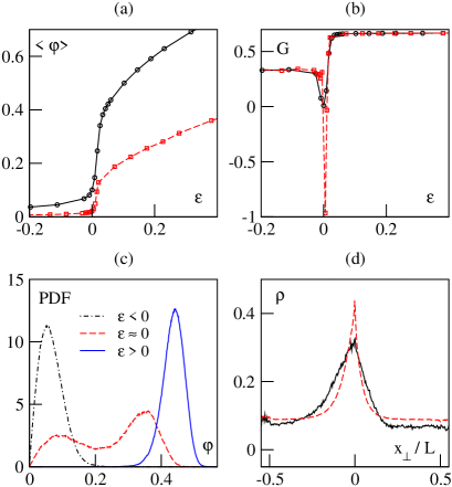
Figure 2: Numerical simulations with multiple-particle interactions, from Gregoire04 (dashed line in (a), (b) and (d)) and with binary collisions (full line). (a) average order parameter; (b) Binder cumulant; (c) distribution of the order parameter for binary collisions; (d) density profile along the coordinate $x_{\perp}$.

Binary versus multiple-particle interactions.– To confirm that binary collisions are sufficient to capture the phenomena reported in numerical simulations Vicsek ; Gregoire04 , we performed numerical simulations of a model with binary collisions , and compared them with results obtained in a model with multi-particle interactions Gregoire04 . In both models, $N$ particles evolve on a periodic domain of linear size $L$, with the same density $\rho_{0}=N/L^{2}=\frac{1}{8}$ in natural microscopic units ($L=256$ for the binary collisions model, and $L=512$ for the other model). The order parameter $\langle\varphi\rangle$, where $\varphi=N^{-1}|\sum_{j=1}^{N}e^{i\theta_{j}}|$, is shown on Fig. 2(a) as a function of the reduced noise $\varepsilon=(\tilde{\sigma}_{t}-\tilde{\sigma})/\tilde{\sigma}_{t}$, $\tilde{\sigma}^{2}$ being the variance of the noise, and $\tilde{\sigma}_{t}$ the value of $\tilde{\sigma}$ at the transition. Fig. 2(b) shows the Binder cumulant $G=1-\langle\varphi^{4}\rangle/3\langle\varphi^{2}\rangle^{2}$. The negative peak indicates a discontinuous transition toward spontaneous motion, which is confirmed in Fig. 2(c) by plotting the probability distribution function (PDF) of the order parameter (for binary collisions) for $\varepsilon$ below, above and very close to the transition . The distribution is clearly bimodal at the transition, which is typical of discontinuous transitions. Finally, Fig. 2(d) presents the density profile obtained when spontaneous motion sets in, indicating the presence of a stripe with higher density. This stripe is essentially invariant along the $x_{\|}$ direction, and is moving along the $x_{\perp}$ direction (on which the profile is measured, using a moving frame). Note that the profile is asymmetric, with a higher slope on the front. Thus, a model with only binary collisions is legitimate and behaves qualitatively in a similar way as a model with more complicated interactions.

Boltzmann equation.– The Boltzmann equation describing the evolution of the one-particle phase-space distribution $f(\mathbf{r},\theta,t)$ reads

$$\frac{\partial f}{\partial t}(\mathbf{r},\theta,t)+\mathbf{e}(\theta)\cdot\nabla f(\mathbf{r},\theta,t)=I_{\text{dif}}[f]+I_{\text{col}}[f]$$ (1)

where $I_{\text{dif}}[f]$ accounts for the self-diffusion phenomenon, and $I_{\text{col}}[f]$ describes the effect of collisions; $\mathbf{e}(\theta)$ is the unit vector in the direction $\theta$. $I_{\text{dif}}[f]$ is given by

$$I_{\text{dif}}[f] = -\lambda f(\mathbf{r},\theta,t)+\lambda\int_{-\pi}^{\pi}d\theta^{\prime}\int_{-\infty}^{\infty}d\eta\,p_{0}(\eta)$$

$$\quad\times\sum_{m=-\infty}^{\infty}\delta(\theta^{\prime}+\eta-\theta+2m\pi)f(\mathbf{r},\theta^{\prime},t)$$

The collision term $I_{\text{col}}[f]$ is evaluated as follows. By definition, two particles collide if their relative distance becomes less than $d_{0}$. In the referential of particle $1$, particle $2$ has a velocity $\mathbf{v}_{2}^{\prime}=\mathbf{e}(\theta_{2})-\mathbf{e}(\theta_{1})$. Thus, particles that collide with particle $1$ between $t$ and $t+dt$ are those that lie, at time $t$, in a rectangle of length $|\mathbf{v}_{2}^{\prime}|$ and of width $2d_{0}$. This leads to

$$I_{\text{col}}[f] = -f(\mathbf{r},\theta,t)\int_{-\pi}^{\pi}d\theta^{\prime}\,|\mathbf{e}(\theta^{\prime})-\mathbf{e}(\theta)|f(\mathbf{r},\theta^{\prime},t)$$

$$+ \int_{-\pi}^{\pi}d\theta_{1}\int_{-\pi}^{\pi}d\theta_{2}\int_{-\infty}^{\infty}d\eta\,p(\eta)\,|\mathbf{e}(\theta_{2})-\mathbf{e}(\theta_{1})|$$

$$\times f(\mathbf{r},\theta_{1},t)f(\mathbf{r},\theta_{2},t)\sum_{m=-\infty}^{\infty}\delta(\overline{\theta}+\eta-\theta+2m\pi)$$

with $\overline{\theta}=\text{Arg}(e^{i\theta_{1}}+e^{i\theta_{2}})$. It can be checked easily that the uniform distribution $f(\mathbf{r},\theta,t)=\rho/2\pi$, is a solution of Eq. (1) for any density, and whatever the form of the noise distributions $p_{0}(\eta)$ and $p(\eta)$.

Hydrodynamic equations.– Let us now define the hydrodynamic density and velocity fields $\rho(\mathbf{r},t)$ and $\mathbf{u}(\mathbf{r},t)$

$$\rho(\mathbf{r},t) = \int_{-\pi}^{\pi}d\theta\,f(\mathbf{r},\theta,t)$$ (4)

$$\rho(\mathbf{r},t)\,\mathbf{u}(\mathbf{r},t) = \int_{-\pi}^{\pi}d\theta\,f(\mathbf{r},\theta,t)\,\mathbf{e}(\theta)$$ (5)

Integrating the Boltzmann equation (1) over $\theta$ yields the continuity equation for $\rho(\mathbf{r},t)$

$$\frac{\partial\rho}{\partial t}+\nabla\cdot(\rho\mathbf{u})=0$$ (6)

The derivation of a hydrodynamic equation for the velocity field is less straightforward, and involves an approximation scheme. Let us introduce the Fourier series expansion of $f(\mathbf{r},\theta,t)$ with respect to $\theta$

$$\hat{f}_{k}(\mathbf{r},t)=\int_{-\pi}^{\pi}d\theta\,f(\mathbf{r},\theta,t)\,e^{ik\theta}$$ (7)

Multiplying Eq. (1) by $e^{ik\theta}$ and integrating over $\theta$ leads to an infinite set of coupled equations for $\hat{f}_{k}(\mathbf{r},t)$. We note that, identifying complex numbers with two-dimensional vectors so that $e^{i\theta}$ corresponds to $\mathbf{e}(\theta)$, the Fourier coefficient $\hat{f}_{1}(\mathbf{r},t)$ is nothing but the “momentum” field $\mathbf{w}(\mathbf{r},t)=\rho(\mathbf{r},t)\,\mathbf{u}(\mathbf{r},t)$. Thus the evolution equation for $\hat{f}_{1}(\mathbf{r},t)$ should yield the hydrodynamic equation for $\mathbf{u}(\mathbf{r},t)$. Yet, as $\hat{f}_{k}(\mathbf{r},t)$ is coupled to all others $\hat{f}_{l}(\mathbf{r},t)$, a closure relation has to be found. In the following, we assume that the velocity distribution $f(\mathbf{r},\theta,t)$ is only slightly non-isotropic, or in other words that $\mathbf{u}(\mathbf{r},t)$ is small as compared to the individual velocity of particles, and that the hydrodynamic fields vary on length scales that are much larger than the microscopic length $d_{0}$. As a result, the velocity equation is obtained from the equation for $\hat{f}_{1}$ through an expansion to leading orders in $\hat{f}_{k}(\mathbf{r},t)$ and in space and time derivatives. Noting that $\hat{f}_{0}(\mathbf{r},t)=\rho(\mathbf{r},t)=\mathcal{O}(1)$, we set $\hat{f}_{1}(\mathbf{r},t)=\mathcal{O}(\epsilon)$, $\epsilon\ll 1$. A consistent scaling ansatz, confirmed by a numerical integration of Eq. (1) in the steady state, is $\hat{f}_{k}(\mathbf{r},t)=\mathcal{O}(\epsilon^{|k|})$. Expanding to order $\epsilon^{3}$, one only keeps the terms in $\hat{f}_{1}$ and $\hat{f}_{2}$ in the evolution equation for $\hat{f}_{1}$. A similar expansion of the equation for $\hat{f}_{2}$ leads to a closure relation for the equation on $\hat{f}_{1}$, finally leading to the following hydrodynamic equation long

$$\frac{\partial\mathbf{w}}{\partial t}+\gamma(\mathbf{w}\cdot\nabla)\mathbf{w} = -\frac{1}{2}\nabla(\rho-\kappa\mathbf{w}^{2})$$

$$+ (\mu-\xi\mathbf{w}^{2})\mathbf{w}+\nu\nabla^{2}\mathbf{w}-\kappa(\nabla\cdot\mathbf{w})\mathbf{w}$$

where the different coefficients are given by

$$\nu = \frac{1}{4}\left[\lambda\left(1-e^{-2\sigma_{0}^{2}}\right)+\frac{4}{\pi}\rho\left(\frac{14}{15}+\frac{2}{3}e^{-2\sigma^{2}}\right)\right]^{-1}$$ (9)

$$\gamma = \frac{8\nu}{\pi}\left(\frac{16}{15}+2e^{-2\sigma^{2}}-e^{-\sigma^{2}/2}\right)$$ (10)

$$\kappa = \frac{8\nu}{\pi}\left(\frac{4}{15}+2e^{-2\sigma^{2}}+e^{-\sigma^{2}/2}\right)$$ (11)

$$\mu = \frac{4}{\pi}\rho\left(e^{-\sigma^{2}/2}-\frac{2}{3}\right)-\lambda\left(1-e^{-\sigma_{0}^{2}/2}\right)$$ (12)

$$\xi = \frac{64\nu}{\pi^{2}}\left(e^{-\sigma^{2}/2}-\frac{2}{5}\right)\left(\frac{1}{3}+e^{-2\sigma^{2}}\right)$$ (13)

The first term in the r.h.s. of Eq. (Boltzmann and hydrodynamic description for self-propelled particles) may be thought of as a pressure gradient, introducing an effective pressure $p=\frac{1}{2}(\rho-\kappa\mathbf{w}^{2})$. The second term describes the local relaxation of $\mathbf{w}$, whereas the third term corresponds to the usual viscous term, and the last one may be interpreted as a feedback from the compressibility of the flow. The fact that $\gamma\neq 1$ (apart from special values of $\sigma$) in the advection term expresses that the problem is not Galilean invariant. Note that $\nu$, $\gamma$ and $\kappa$ are always positive; $\mu$ can change sign, and $\xi>0$ whenever $\mu>0$. All the terms are compatible with the phenomenological equation of motion of Toner et al. Toner . However, our approach provides explicit forms for the coefficients. In particular, the coefficient in front of the term $\nabla(\nabla\cdot\mathbf{w})$ is strictly zero in our case. Besides, there is no term of the form ${(\mathbf{w}\cdot\nabla)}^{2}\mathbf{w}$ due to the order of truncation of the Boltzmann equation.

Phase diagram.– We can now study the spontaneous onset of collective motion in the present model. As a first step, it is interesting to consider possible instabilities of the spatially homogeneous system, that is the appearance of a uniform nonzero field $\mathbf{w}$. Equating all space derivatives to zero leads to the simple equation

$$\frac{\partial\mathbf{w}}{\partial t}=(\mu-\xi\mathbf{w}^{2})\mathbf{w}$$ (14)

Clearly, $\mathbf{w}=0$ is solution for all values of the coefficients, but it becomes unstable for $\mu>0$, when a nonzero solution $\mathbf{w}_{0}=\sqrt{\mu/\xi}\,\mathbf{e}$ appears, where $\mathbf{e}$ is an arbitrary unit vector. From Eq. (12), the value $\mu=0$ corresponds to a threshold value $\rho_{t}$

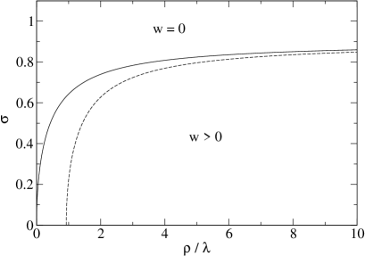
Figure 3: Phase diagram of the model in the plane $(\rho/\lambda,\sigma)$. A transition line (full line: $\sigma_{0}=\sigma$; dashed line: $\sigma_{0}=1$) indicates the linear instability threshold of the state $w=|\mathbf{w}|=0$.

$$\rho_{t}=\frac{\pi\lambda(1-e^{-\sigma_{0}^{2}/2})}{4(e^{-\sigma^{2}/2}-\frac{2}{3})}$$ (15)

The transition line defined by $\rho_{t}$ in the plane $(\rho/\lambda,\sigma)$ is plotted on Fig. 3, for $\sigma_{0}=\sigma$ and for a fixed value $\sigma_{0}=1$. If $\sigma_{0}=\sigma$, the instability occurs at any density, provided the noise is low enough. On the contrary, at fixed $\sigma_{0}$, the instability disappears below a finite density $\rho_{t}^{0}=3\pi\lambda(1-e^{-\sigma_{0}^{2}/2})/4$. Both transition lines saturate at a value $\sigma_{t}=(2\ln\frac{3}{2})^{1/2}\approx 0.90$.

Let us now test the stability against perturbations of the above spatially homogeneous flow $\mathbf{w}(\mathbf{r},t)=\mathbf{w}_{0}$, with finite density $\rho_{0}$, in an infinite space. From Eq. (14), it is clear that $\mathbf{w}_{0}$ is stable against spatially homogeneous perturbations. Yet, this solution may be unstable against finite wavelength perturbations . To check this issue, we introduce a perturbation around the homogeneous steady-state solution

$$\rho(\mathbf{r},t)=\rho_{0}+\delta\rho(\mathbf{r},t),\quad\mathbf{w}(\mathbf{r},t)=\mathbf{w}_{0}+\delta\mathbf{w}(\mathbf{r},t)$$ (16)

and linearize Eq. (Boltzmann and hydrodynamic description for self-propelled particles) in $\delta\rho(\mathbf{r},t)$ and $\delta\mathbf{w}(\mathbf{r},t)$. Linear stability is then tested with the ansatz

$$\delta\rho(\mathbf{r},t)=\delta\rho_{0}\,e^{st+i\mathbf{q}\cdot\mathbf{r}},\quad\delta\mathbf{w}(\mathbf{r},t)=\delta\mathbf{w}_{0}\,e^{st+i\mathbf{q}\cdot\mathbf{r}},$$ (17)

where $\mathbf{q}$ is a given wavevector, by looking for the dispersion relation $s(\mathbf{q})$. By choosing $\delta\mathbf{w}_{0}$ and $\mathbf{q}$ along the same direction as $\mathbf{w}_{0}$, one finds for the real part of $s$

$$\Re(s)=\frac{\mu_{0}^{2}}{8\,\xi^{3}w_{0}^{4}}\,|\mathbf{q}|^{2}-\frac{5\,\mu_{0}^{4}}{128\,\xi^{7}w_{0}^{10}}\,|\mathbf{q}|^{4}+\mathcal{O}(|\mathbf{q}|^{6})$$ (18)

for small $|\mathbf{q}|$, with $\mu_{0}=4(e^{-\sigma^{2}/2}-\frac{2}{3})/\pi$ and $w_{0}=|\mathbf{w}_{0}|$, indicating the onset of a long wavelength instability since $\Re(s)$ becomes positive at small enough $|\mathbf{q}|$ . The spatially homogeneous states $\mathbf{w}=0$ and $\mathbf{w}=\mathbf{w}_{0}$ are thus both unstable, so that more complicated structures should eventually appear in the system. The “stripes” of higher density moving over a low density background, reported in Gregoire04 , may be examples of such patterns. Physically, the instability may be interpreted as follows: if locally $\rho>\rho_{0}$ ($\rho<\rho_{0}$), the local velocity $\mathbf{u}$ increases (decreases), creating velocity gradients that generate a density wave. Note that the perturbations that destabilize the long-range order correspond to longitudinal waves, at odds with what happens in the two-dimensional XY-model Kosterlitz which might be thought of as an equilibrium counterpart of the present model Toner .

Discussion.– Our analytical approach has several advantages when compared with pure numerical simulations of similar microscopic models. First, the hydrodynamic equations may be used to get analytical solutions in reference cases with simple geometries, and to analyze their stability against perturbations. Second, in more complicated situations, these equations may be integrated numerically, allowing one to study much larger systems than with direct simulations of the particles.

The hydrodynamic equations (6,Boltzmann and hydrodynamic description for self-propelled particles) have been derived from a Boltzmann approach and their validity is in principle restricted to a low density regime (note that the transition may occur at low density by choosing $\lambda\ll 1$). However, as verified for many systems, the validity of the Boltzmann equation often goes well-beyond the a priori expected limit. One also expects that in this low density regime, the hydrodynamic equations should not depend strongly on the details of the interactions, as the shape of $p(\eta)$. Another limitation comes from the assumption that $\mathbf{w}$ is small. This assumption is valid to describe the evolution of small perturbations around the zero velocity state. When crossing the transition line, the assumption is self-consistent, as the resulting homogeneous velocity field grows continuously from zero. Yet, the finite-wavelength instability may drive the system into a regime where the approximation is no longer valid. Checking this point requires to find the structures emerging from Eqs. (6,Boltzmann and hydrodynamic description for self-propelled particles), and to compare them with numerical simulations. Work in this direction is under investigation long .

Acknowledgments.– G.G. is grateful to H. Chaté for introducing him to this subject. This work has been partly supported by the Swiss National Science Foundation.

References

- (1) J.K. Parrish and W.M. Hamner (Eds.), Three Dimensional Animals Groups, Cambridge University Press (Cambridge, 1997).
- (2) J.T. Bonner, Proc. Natl. Acad. Sci. USA 95, 9355 (1998); M.T. Laub and W.F. Loomis, Mol. Bio. of the Cell 9, 3521 (1998).
- (3) D. Helbing, I. Farkas, and T. Vicsek, Nature (London) 407, 487 (2000); Phys. Rev. Lett. 84, 1240 (2000).
- (4) Y. Harada, A. Nogushi, A. Kishino, and T. Yanagida, Nature (London) 326, 805 (1987); M. Badoual, F. Jülicher and J. Prost, Proc. Natl. Acad. Sci. USA 99, 6696 (2002).
- (5) K. Sugawara, M. Sano, and T. Watanabe, Proc. of 2002 FIRA Robot World Congress, p.36 (2002).
- (6) N. Shimoyama et al., Phys. Rev. Lett. 76, 3870 (1996); G. Flierl et al., J. Theor. Biol. 196, 397 (1999); A. S. Mikhailov and D. H. Zanette, Phys. Rev. E 60, 4571 (1999); H. Levine, W.-J. Rappel, and I. Cohen, Phys. Rev. E 63, 017101 (2001).
- (7) J. Toner, Y. Tu, and S. Ramaswamy, Ann. Phys. 318, 170 (2005).
- (8) T. Vicsek, A. Czirók, E. Ben-Jacob, I. Cohen, and O. Shochet, Phys. Rev. Lett. 75, 1226 (1995); A. Czirók, H. Stanley, and T. Vicsek, J. Phys. A 30, 1375 (1997).
- (9) G. Grégoire, H. Chaté, and Y. Tu, Physica D 181, 157 (2003).
- (10) G. Grégoire and H. Chaté, Phys. Rev. Lett. 92, 025702 (2004).
- (11) Z. Csahók and T. Vicsek, Phys. Rev. E 52, 5297 (1995).
- (12) M. Aldana and C. Huepe, J. Stat. Phys. 112, 135 (2003).
- (13) H. J. Bussemaker, A. Deutsch, and E. Geigant, Phys. Rev. Lett. 78, 5018 (1997).
- (14) J. Toner and Y. Tu, Phys. Rev. Lett. 75, 4326 (1995); Phys. Rev. E 58, 4828 (1998); Y. Tu, J. Toner, and M. Ulm, Phys. Rev. Lett. 80, 4819 (1998).
- (15) R. A. Simha and S. Ramaswamy, Phys. Rev. Lett. 89, 058101 (2002); Physica A 306, 262 (2002).
- (16) Z. Csahók and A. Czirók, Physica A 243, 304 (1997).
- (17) D. Mermin and H. Wagner, Phys. Rev. Lett. 17, 1133 (1966).
- (18) E. Bertin, M. Droz, and G. Grégoire, to be published.
- (19) J. M. Kosterlitz and D. J. Thouless, J. Phys. C 6, 1181 (1973).