An exact Coulomb cutoff technique for supercell calculations

Abstract

We present a new reciprocal space analytical method to cutoff the long range interactions in supercell calculations for systems that are infinite and periodic in 1 or 2 dimensions, extending previous works for finite systems. The proposed cutoffs are functions in Fourier space, that are used as a multiplicative factor to screen the bare Coulomb interaction. The functions are analytic everywhere but in a sub-domain of the Fourier space that depends on the periodic dimensionality. We show that the divergences that lead to the non-analytical behaviour can be exactly cancelled when both the ionic and the Hartree potential are properly screened. This technique is exact, fast, and very easy to implement in already existing supercell codes. To illustrate the performance of the new scheme, we apply it to the case of the Coulomb interaction in systems with reduced periodicity (as one-dimensional chains and layers). For those test cases we address the impact of the cutoff in different relevant quantities for ground and excited state properties, namely: the convergence of the ground state properties, the static polarisability of the system, the quasiparticle corrections in the GW scheme and in the binding energy of the excitonic states in the Bethe-Salpeter equation. The results are very promising.

I Introduction

Plane waves expansions with periodic boundary conditions have been proven to be a very effective way to exploit the translational symmetry of infinite crystal solids, in order to calculate the properties of the bulk, by performing the simulations in one of its primitive cells only pw . The use of plane waves is motivated by several facts. First, the translational symmetry of the potentials involved in the calculations is naturally and easily accounted for in reciprocal space, through the Fourier expansion. Second, very efficient and fast algorithms exist (like FFTWfftw ) that allow us to calculate the Fourier transforms very efficiently. Third the expansion in plane waves is exact, since they form a complete set, and it is only limited in practice by one parameter, namely, the maximum value of the momentum, that determines the size of the chosen set. Fourth, in many cases, the use of Born-von Karmán periodic boundary conditions supplies a conceptually easy (though artificial) way to get rid of the dependence of the properties of a specific sample on its surface and shape, allowing us to concentrate on the bulk properties of the system in the thermodynamic limit.Lebowitz69

However, mainly in the last decade, increasing interest has been developed in systems at the nano-scale, like tubes, wires, quantum-dots, biomolecules, etc., whose physical dimensionality is, for all practical purposes, less than three.nano These systems are still 3-dimensional (3D), but their quantum properties are those of a confined system in one or more directions, and those of a periodic extended system in the remaining directions. Other classes of systems with the same kind of reduced periodicity are the classes of the polymers, and of the solids with defects.

Throughout this paper we call nD-periodic a 3D object, that can be considered infinite and periodic in $n$ dimensions, being finite in the remaining $3-n$ dimensions. In order to simulate this kind of systems, a commonly adopted approach is the supercell approximation.pw

In the supercell approximation the physical system is treated as a fully 3D-periodic one, but a new unit cell (the supercell) is built in such a way that some extra empty space separates the periodic replica along the direction(s) in which the system is to be considered as finite. This method makes possible to retain all the advantages of plane waves expansions and periodic boundary conditions. Yet the use of a supercell to simulate objects that are not infinite and periodic in all the directions, leads to artifacts, even if a very large portion of vacuum is interposed between the replica of the system in the non-periodic dimensions.

In fact, the straightforward application of the supercell method generates in any case fake images of the original system, that can mutually interact in several ways, affecting the results of the simulation. It is well known that the response function of an overall neutral solid of molecules is not equal, in general, to the response of the isolated molecule, and converges very slowly to it, when the amount of vacuum in the supercell is progressively increased.Onida02 ; ijm

For instance, the presence of higher order multipoles can make undesired images interact via the long range part of the Coulomb potential. In the dynamic regime, multipoles are always generated by the oscillations of the charge density even in systems whose unit cell does not carry any multipole in its ground state. This is the case, for example, when we investigate the response of a system in presence of an external oscillating electric field.

Things go worse when the unit cell carries a net charge, since the total charge of the infinite system represented by the supercell is actually infinite, while the charges at the surfaces of a finite, though very large system always generate a finite polarisation field. This situation is usually normalised in the calculation by the introduction of a suitable compensating positive background charge.

Another common situation in which the electrostatics is known to modify the ground state properties of the system occurs when a layered system is studied, and an infinite array of planes is considered instead of a single slab, being in fact equivalent to an effective chain of capacitors.Wood04

These issues become particularly evident in all the approaches that imply the calculation of non-local operators or response functions, because, in these cases, two supercells may effectively interact even if their charge densities do not overlap at all. This is the case, for example, of the many-body perturbation theory calculations (MBPT), and, in particular, of the self-energy calculations at the GW level.GW ; Onida02

However we are usually still interested in the dispersion relations of the elementary excitations of the system along its periodic directions, and those are ideally dealt with using a plane waves approach. Therefore, the ideal path to keep the advantages of the supercell formulation in plane waves, and to gain a description of systems with reduced periodicity free of spurious effects is to develop a technique to cut the Coulomb interaction off out of a desired region. This problem is not new and has been addressed now for a very long time and in different fields (condensed matter, classical fields, astrophysics, biology, etc). Several different approaches have been proposed in the past to solve it, however a complete review of them is beyond the scope of this paper. The aim of the present work is to focus on the widely used supercell schemes to show how the image interaction influences both the electronic ground state properties and the dynamical screening in the excited state of 0D-, 1D-, 2D-periodic systems, and to propose an exact method to avoid the undesired interaction of the replicas in the non-periodic directions.

The paper is organised as follows: in Sec. II the basics of the plane wave method for solids are reviewed, in Sec. III the new method is outlined, in Sec. IV the treatment of the singularities is explained, in Sec. V some applications of the proposed technique are discussed.

II The 3D-periodic case

The main problem of electrostatics we are facing here can be reduced to the problem of finding solutions to the Poisson equation for a given charge distribution $n(\mathbf{r})$, and given boundary conditions

$$\nabla^{2}V(\mathbf{r})=-4\pi n(\mathbf{r}).$$ (1)

In a finite system the potential is usually required to be zero at infinity. In a periodic system this condition is meaningless, since the system itself extends to infinity. Nevertheless the general solution of Eq. (1) in both cases is known in the form of the convolution

$$V(\mathbf{r})=\iiint_{space}\frac{n(\mathbf{r^{\prime}})}{|\mathbf{r}-\mathbf{r^{\prime}}|}\mathrm{d}^{3}\mathbf{r}^{\prime},$$ (2)

that it is referred from now on as the Hartree potential.

It might seem that the most immediate way to build the solution potential for a given charge distribution is to compute the integral in real space, but problems immediately arise for infinite systems. In fact, the density can be reduced to an infinite sum over delta charge distributions $q\delta(\mathbf{r}-\mathbf{r^{\prime}})$,

$$V(\mathbf{r})=\sum_{\mathbf{n}}\frac{q}{|\mathbf{r}-\mathbf{L}_{\mathbf{n}}|},$$ (3)

and the integral in Eq. (2) becomes an infinite sum as well, but this sum is in general only conditionally, and not absolutely convergent.Makov95 The sum of Eq. (3) a potential that is determined up to a constant for a neutral cell with zero dipole moment, while the corresponding sum for the electric field is absolutely convergent. A neutral cell with a non null dipole moment, on the opposite, gives a divergent potential, and an electric field that is determined up to an unknown constant electric field (the sum for the electric field is conditionally convergent in this case).

Even if, in principle, the surface terms have to be always taken into account, in practice they are only relevant when we want to calculate energy differences between states with different total charge. These terms can be neglected in the case of a neutral cell whose lowest nonzero multipole is quadrupoleDeLeeuw80 . As in the present work we are interested in macroscopic properties of the periodic system, those surface effects are never considered in the discussion that follows. However this sample-shape effects play an important role for the analysis of different spectroscopies as, for example, infrared and nuclear magnetic resonance.

A major source of computational problems is the fact that the sum in Eq. (3) is very slowly converging when it is summed in real space, and this fact has historically motivated the need for reciprocal space methods to calculate it. It was Ewald who first discovered that, by means of an integral transform, the sum can be split in two terms, and that if one is summed in real, while the other in reciprocal space, both of them are rapidly converging.Ewald21 The point of splitting is determined by an arbitrary parameter.

Let us now focus on methods of calculating the sum in Eq. (3) purely based on the reciprocal space.

If we consider a periodic distribution of charges with density $n(\mathbf{r})$ such that $n(\mathbf{r})=n(\mathbf{r}+\mathbf{L_{\mathbf{n}}})$, with $\mathbf{L_{\mathbf{n}}}=\{n_{x}\mathbf{L}_{x},n_{y}\mathbf{L}_{y},n_{z}\mathbf{L}_{z}\}$, and $\{n_{x},n_{y},n_{z}\}\in\mathbb{Z}$, it turns out that the reciprocal space expression for a potential like

$$V(\mathbf{r})=\iiint_{space}n(\mathbf{r^{\prime}})v(|\mathbf{r}-\mathbf{r^{\prime}}|)\mathrm{d}^{3}\mathbf{r}^{\prime},$$ (4)

in a 3D-periodic system, can be written as

$$V(\mathbf{G_{\mathbf{n}}})=n(\mathbf{G_{\mathbf{n}}})v(\mathbf{G}_{\mathbf{n}}),$$ (5)

where we have used the convolution theorem to transform the real space convolution of the density and the Coulomb potential into the product of their reciprocal space counterparts. Here $\mathbf{G_{\mathbf{n}}}=\{n_{x}\mathbf{G}_{x},n_{y}\mathbf{G}_{y},n_{z}\mathbf{G}_{z}\}$ are the multiples of the primitive reciprocal space vectors $\frac{2\pi}{\mathbf{L_{\mathbf{n}}}}$, and $v(\mathbf{G}_{\mathbf{n}})$ is the Fourier transform of the long range interaction $v(\mathbf{r})$, evaluated at the point $\mathbf{G}_{\mathbf{n}}$. For the Coulomb potential it is

$$v(\mathbf{G_{\mathbf{n}}})=\frac{4\pi}{G_{\mathbf{n}}^{2}}.$$ (6)

Fourier transforming expression (5) back into real space we have, for a unit cell of volume $\Omega$,

$$V(\mathbf{r})=\frac{4\pi}{\Omega}\sum_{\mathbf{n}\neq 0}\frac{n(\mathbf{G_{\mathbf{n}}})}{G_{\mathbf{n}}^{2}}\exp(i\mathbf{G_{\mathbf{n}}}\cdot\mathbf{r}).$$ (7)

At the singular point $n_{x}=n_{y}=n_{z}=0$ the potential $V$ is undefined, but, since the value at $G=0$ corresponds to the average value of $V$ in real space, it can be chosen to be any number, corresponding to the arbitrariness in the choice of the static gauge (a constant) for the potential. Observe that the same expression can be adopted in the case of a charged unit cell, but this time, the arbitrary choice of $v(G)$ in $G=0$ corresponds to the use of a uniform background neutralising charge.

III Systems with reduced periodicity

It has been shownSphor94 that the slab capacitance effect mentioned in the introduction actually is a problem that cannot be solved by just adding more vacuum to the supercell. This has initially led to the development of corrections to Ewald’s original methodYeh99 , and then to rigorous extensions in 2D and 1D.Martyna99 ; Brodka03 The basic idea is to restrict the sum in reciprocal space to the reciprocal vectors that actually correspond to the periodic directions of the system. These approach are in general of order $O(N^{2})$Heyes77 ; Grzybowski00 , but they have been recently refined to order $O(N\ln N)$.Minary02 ; Minary04 Another class of techniques, developed so far for finite systems, is based on the expansion of the interaction into a series of multipoles (fast multipole method).fmm ; Castro03 ; fmm-perio With this technique it is possible to evaluate effective boundary conditions for the Poisson’s equations at the cell’s boundary, so that the use of a supercell is not required at all, making it computationally very efficient for finitefmm ; Castro03 and extended systemsfmm-perio . Other known methods, tipically used in molecular dynamics simulations, are the multipole-correction methodSchultz99 , and the particle-mesh methodHockney , whose review is beyond the scope of the present work, and we refer the reader to the original works for details.

Differently from what happens for the Ewald sum, the method that we propose to evaluate the sum in Eq. (3) entirely relies on the Fourier space and amounts to screening the unit cell from the undesired effect of (some of) its periodic images. The basic expression is Eq. (5), whose accuracy is only limited by the maximum value $G_{N}$ of the reciprocal space vectors in the sum. Since there is no splitting between real and reciprocal space, no convergence parameters are required.

Our goal is to transform the 3D-periodic Fourier representation of the Hartree potential of Eq. (5) into the modified one

$$\tilde{V}(\mathbf{\mathbf{G}_{\mathbf{n}}})=\tilde{n}(\mathbf{G_{\mathbf{n}}})\tilde{v}(\mathbf{G}_{\mathbf{n}})$$ (8)

such that all the interactions among the undesired periodic replica of the system disappear. The present method is a generalisation of the method proposed by Jarvis et al.Jarvis97 for the case of a finite system.

In order to build this representation, we want to: 1) define a screening region $\cal D$ around each charge in the system, out of which there is no Coulomb interaction; 2) calculate the Fourier transform of the desired effective interaction $\tilde{v}(r)$ that equals the Coulomb potential in $\cal{D}$, and is $0$ outside $\cal{D}$

$$\tilde{V}(r)=\begin{cases}\frac{1}{r}&\text{if $r\in\cal{D}$}\\ 0&\text{if $r\notin\cal{D}$}\end{cases}.$$ (9)

Finally we must 3) modify the density $n(\mathbf{r})$ in such a way that the effective density is still 3D-periodic, so that the convolution theorem can be still applied, but densities belonging to undesired images are not close enough to interact through $\tilde{v}(r)$.

The choice of the region $\cal{D}$ for step 1) is suggested by symmetry considerations, and it is a sphere (or radius $R$) for finite systems, an infinite cylinder (of radius $R$) for 1D-periodic systems, and an infinite slab (of thickness $2R$) for 2D-periodic systems.

Step 2) means that we have to calculate the modified Fourier integral

$$\tilde{V}(\mathbf{G})=\iiint_{space}\tilde{v}(r)\mathrm{e}^{-i\mathbf{G}\cdot\mathbf{r}}\mathrm{d}^{3}\mathbf{r}=\iiint_{\cal D}v(r)\mathrm{e}^{-i\mathbf{G}\cdot\mathbf{r}}\mathrm{d}^{3}\mathbf{r}.$$ (10)

Still we have to avoid that two neighbouring images interact by taking them far away enough from each other. Then step 3) means that we have to build a suitable supercell, and re-define the density in it.

Let us examine first step 2), i.e. the cutoff Coulomb interaction in reciprocal space. We know the expression of the potential when it is cutoff in a sphere.Jarvis97 It is

$$\tilde{v}^{0D}(G)=\frac{4\pi}{G^{2}}\bigl{[}1-\cos(GR)\bigr{]}.$$ (11)

The limit $R\to\infty$ converges to the bare Coulomb term in the sense of a distribution, while, since $\lim_{G\to 0}\tilde{v}^{0D}(G)=2\pi R^{2}$, there is no particular difficulty in the origin. This scheme has been successfully used in many applicationsMakov95 ; Jarvis97 ; Castro03 ; octopus ; Onida95 .

The 1D-periodic case applies to systems with infinite extent in the $x$ direction, and finite in the $y$ and $z$ directions. The effective Coulomb interaction is then defined in real space to be $0$ out of a cylinder of radius $R$ having its axis parallel to the $x$ direction. By performing the Fourier transformation we get the following expression for the cutoff coulomb potential in cylindrical coordinates:Gradshteyn

$$\tilde{v}^{1D}(G_{x},G_{\bot})=\frac{4\pi}{G^{2}}\bigg{[}1+G_{\bot}RJ_{1}(G_{\bot}R)K_{0}(|G_{x}|R)\\ -|G_{x}|RJ_{0}(G_{\bot}R)K_{1}(|G_{x}|R)\bigg{]},$$ (12)

where $J$ and $K$ are the ordinary and modified cylindrical Bessel functions, and $G_{\bot}=\sqrt{G_{y}^{2}+G_{z}^{2}}$.

It is easy to realise that, since the $K$ functions damp the oscillations of the $J$ functions very quickly, for all practical purposes this cutoff function only acts on the very first smaller values of $G$, while the unscreened $\frac{4\pi}{G^{2}}$ behaviour is almost unchanged for the larger values.

Unfortunately, while the $J_{n}(\xi)$ functions have a constant value for $\xi=0$, and the whole cutoff is well defined for $G_{\bot}=0$, the $K_{0}(\xi)$ function diverges logarithmically for $\xi\to 0$. Since, on the other hand, $K_{1}(\xi)\approx\xi^{-1}$ for small $\xi$,

$$\tilde{v}^{1D}(G_{x},G_{\bot})\sim-\log(G_{x}R)\quad\textrm{for $G_{\bot}>0$, $G_{x}\to 0^{+}$}.$$ (13)

This means that the limit $\lim_{G\to 0^{+}}v(G)$ does not exist for this cutoff function, and the whole $G_{x}=0$ plane is ill-defined. We will come back to the treatment of the singularities in the next section. We notice that this logarithmic divergence is the common dependence one would get for the electrostatic potential of a uniformly charged 1D wireJackson . It is expected that bringing charge neutrality in place would cancel this divergence (see below).

The 2D-periodic case, with finite extent in the $z$ direction, is calculated in a similar manner. The effective Coulomb interaction is defined in real space to be $0$ out of a slab of thickness $2R$ symmetric with respect to the $xy$ plane. In Cartesian coordinates we get

$$\tilde{v}^{2D}(G_{\|},G_{z})=\frac{4\pi}{G^{2}}\bigg{[}1 +\mathrm{e}^{-G_{\|}R}\frac{|G_{z}|}{G_{\|}}\sin(|G_{z}|R)$$

$$-\mathrm{e}^{-G_{\|}R}\cos(|G_{z}|R)\bigg{]},$$ (14)

where $G_{\|}=\sqrt{G_{x}^{2}+G_{y}^{2}}$.

In the limit $R\to\infty$ the unscreened potential $\frac{4\pi}{G^{2}}$ is recovered. Similarly to the case of 1D, the limit $G\to 0$ does not exist, since for $G_{z}=0$, the cutoff has a finite value, while it diverges in the limit $G_{\|}\to 0$

$$\tilde{v}^{2D}(G_{\|},G_{z})\sim\frac{1}{G_{\|}^{2}}\quad\textrm{for $G_{\|}>0$, $G_{z}\to 0^{+}$}.$$ (15)

So far we haven’t committed to a precise value of the cutoff length $R$. This value has to be chosen, for each dimensionality, in such a way that it avoids the interaction of any two neighbour images of the unit cell in the non-periodic dimension.

In order to fix the values of $R$ we must choose the size of the supercell. This leads us to the step 3) of our procedure. We recall that even once the long range interaction is cutoff out of some region around each component of the system, this is not sufficient yet to avoid the interaction among undesired images. The charge density has to be modified, or, equivalently, the supercell has to be built in such a way that two neighbouring densities along every non periodic direction do not interact via the cutoff interaction.

It is easy to see how this could happen in the simple case of a 2D square cell of length $L$: if both $\mathbf{r}$ and $\mathbf{r^{\prime}}$ belongs to the cell, then $r,r^{\prime}\leq L$, and $|\mathbf{r}-\mathbf{r^{\prime}}|\leq\sqrt{2}L$ (see the schematic drawing in Fig. 1). If a supercell is built that is smaller than $(1+\sqrt{2})L$, there could be residual interaction, and the cutoff would no longer lead to the exact removal of the undesired interactions.

Let us call $A_{0}$ the unit cell of the system we are working on, and ${\cal A}=\{A_{i},i=-\infty,\cdots,\infty\}$ the set of all the cells in the system. If the system is nD-periodic this set only includes the periodic images of $A_{0}$ in the $n$ periodic directions. Let us call ${\cal B}$ the set of all the non-physical images of the system, i.e. those in the non-periodic directions. Then ${\cal A}\cup{\cal B}=\mathbb{R}^{3}$. Obviously, if the system is 3D-periodic ${\cal A}=\mathbb{R}^{3}$, and ${\cal B}\equiv\varnothing$.

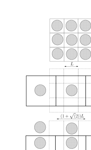
Figure 1: Schematic description for the supercell construction in a 2D system. The upper sketch corresponds to the 2D-periodic case (i.e. a 2D crystal). The middle sketch corresponds to a 0D-periodic system, and the bottom one to a 1D-periodic. In the 0D-periodic case the systems in different cells do not interact, while in the 1D-periodic the chains do not interact, but within each chain the interaction of all of its elements is permitted..

In general we want to allow the interaction of the electrons in $A_{0}$ with the electrons in all the cells $A_{i}\in{\cal A}$, but not with those $B_{i}\in{\cal B}$. To obtain this we define the supercell $C_{0}\supseteq A_{0}$ such that, $\forall i$

$$\begin{cases}\text{if $\mathbf{r}\in A_{0}$, and $\mathbf{r}^{\prime}\in A_{i}$}&\text{then $|\mathbf{r}-\mathbf{r}^{\prime}|\in C_{0}$}\\ \text{if $\mathbf{r}\in A_{0}$, and $\mathbf{r}^{\prime}\in B_{i}$}&\text{then $|\mathbf{r}-\mathbf{r}^{\prime}|\notin C_{0}$}\\ \end{cases}$$ (16)

(see Fig. 1 for a simplified 2D sketch). The new density $\tilde{n}(\mathbf{r})$ is such that

$$\begin{cases}\text{if $\mathbf{r}\in A_{0}$}&\text{then $\tilde{n}(\mathbf{r})=n(\mathbf{r})$,}\\ \text{if $\mathbf{r}\in C_{0}$, and $\mathbf{r}\notin A_{0}$}&\text{then $\tilde{n}(\mathbf{r})=0$.}\\ \end{cases}$$ (17)

The size $L_{C}$ of the super-cell in the non-periodic directions depends on the periodic dimensionality of the system. In order to completely avoid any interaction, even in the case the density of the system is not zero at the cell border, it has to be

$$\begin{cases}\text{$L_{C}=(1+\sqrt{3})L$}&\text{for finite}\\ \text{$L_{C}=(1+\sqrt{2})L$}&\text{for 1D-periodic}\\ \text{$L_{C}=2L$}&\text{for 2D-periodic}\end{cases}$$ (18)

Actually, since the required super-cell is quite large, a compromise between speed and accuracy can be achieved in the computation, using parallelepiped super-cell with $L_{C}=2L$ for all the cases. This approximation rests on the fact that the charge density is usually contained in a region smaller than the cell in the non-periodic directions, so that the spurious interactions are, in fact, avoided, even with a smaller cell. Therefore, on the basis of this approximation, we can choose the value of the cutoff length $R$ always as half the smallest primitive vector in the non-periodic dimension.

IV Cancellation of the singularities

The main point in the procedure of eliminating the divergences in all the cases of interest is to observe that our final goal is usually not to obtain the expression of the Hartree potential alone, because all the physical quantities depend on the total potential, i.e. on the sum of the electronic and the ionic potential. When this sum is considered we can exploit the fact that each potential is defined up to an arbitrary additive constant, and choose the constants consistently for the two potentials. Since we know in advance that the sum must be finite, we can include, so to speak, all the infinities into these constants, provided that we find a method to separate out the long range part of both potentials on the same footing.

In what follows we show how charge neutrality can be exploited to obtain the exact cancellations when operating with the cutoff expression of Sec. III in Fourier space.

The total potential of the system is built in the following way: we separate out first short and long range contributions to the ionic potential by adding and subtracting a Gaussian charge density $n_{+}(r)=Z\exp(-a^{2}r^{2})$. The potential generated by this density is $V_{+}(r)=Z\frac{\mathrm{erf}(ar)}{r}$. The ionic potential is then written as

$$V(r)=\Delta V(r)-Z\frac{\mathrm{erf}(ar)}{r},$$ (19)

where $a$ is chosen so that $\Delta V(r)$ is localised within a sphere of radius $r_{a}$, smaller than the cell size. The expression of the ionic potential in reciprocal space is

$$V(\mathbf{G})=4\pi\left[\int_{0}^{+\infty}\frac{r\sin(Gr)}{G}\Delta V(r)\mathrm{d}r-\frac{\exp\left(-\frac{G^{2}}{4a^{2}}\right)}{G^{2}}\right]$$ (20)

which, for $G=0$ gives a finite contribution from the first term, and a divergent contribution from the second term

$$V(G=0)=4\pi\int_{0}^{+\infty}r^{2}\Delta V(r)\mathrm{d}r-\infty.$$ (21)

The first is the contribution of the localised charge, and is easily computed, since the integrand is zero for $r>r_{a}$. The second term is cancelled by the corresponding $G=0$ term in the electronic Hartree potential, due to the charge neutrality of the system. This trivially solves the problem of the divergences in 3D-periodic systems.

Now let us consider a 1D-periodic system. The Hartree term alone in real space is given by

$$V(x,y,z)=\sum_{G_{x}}\iint_{\Omega}n(G_{x},y^{\prime},z^{\prime})\\ \times v(G_{x},y-y^{\prime},z-z^{\prime})\mathrm{e}^{iG_{x}x^{\prime}}\mathrm{d}y^{\prime}\mathrm{d}z^{\prime}.$$ (22)

Invoking the charge neutrality along the chain axis, we have that the difference between electron and ionic densities satisfies

$$\iint\left[n_{\rm ion}(G_{x}=0,y,z)-n_{\rm el}(G_{x}=0,y,z)\right]\mathrm{d}y\mathrm{d}z=0.$$ (23)

Unfortunately, the cutoff function in Eq. (12) is divergent for $G_{x}=0$. So the effective potential results in an undetermined $0\cdot\infty$ form. However, we can work out an analytical expression for it by defining first a finite cylindrical cutoff, but then bringing the size of the cylinder to infinity. This way, as a first step, we get a new cutoff interaction in a finite cylinder of radius $R$, and length $h$, assuming that $h$ is much larger than the cell size in the periodic direction. In this case the modified finite cutoff potential includes a term

$$\tilde{v}^{1D}(G_{x},r,h)\propto\log\left(\frac{h+\sqrt{h^{2}+r^{2}}}{r}\right),$$ (24)

which, in turn gives, for the particular plane $G_{x}=0$,

$$\tilde{v}^{1D}(G_{x}=0,G_{\bot})\approx-4\pi\int_{0}^{R}rJ_{0}(G_{\bot}r)\log(r)\mathrm{d}r\\ +4\pi R\log(2h)\frac{J_{1}(G_{\bot}R)}{G_{\bot}}.$$ (25)

The effective potential is now split into two terms, but only the second one depends on $h$. The second step is achieved by going to the limit $h\to+\infty$, to obtain the exact infinite cutoff. By calculating this limit, we notice that only the second term in the right hand side of Eq. (25) diverges. This term is the one that can be dropped due to charge neutrality (in fact it has the same form for the ionic and electronic charge densities). Thus, for the cancellation to be effective in a practical implementation, we have to treat on the same way both the ionic and Hartree Coulomb contributions. Of course the first term in the right hand side Eq. (25) has always to be taken into account, affecting both the long and the short range part of the cutoff potentials.

Following this procedure, we are able to get a considerable computational advantage, compared, e.g., to the method originally proposed by Spataru et al.,Spataru04b since our cutoff is just an analytical function of the reciprocal space coordinates, and the evaluation of an integral for every value of $G_{x},G_{\perp}$ is not needed. The cutoff proposed in Ref. Spataru04b, is actually a particular case of our cutoff, obtained by using the finite cylinder for all the components of the ${\mathbf{G}}$ vectors: in this case the quadrature in Eq. (25) has to be evaluated for each $G_{x}$, $G_{y}$, and $G_{z}$, and a convergence study in $h$ is mandatory (see discussion in Sec. V.2, and Fig. 5).

In the 1D-periodic case, the $G=0$ value is now well defined, and it turns out to be $\lim_{G_{\bot}\to 0}\tilde{v}(G_{x},G_{\bot})$

$$\tilde{v}^{1D}(G_{x}=0,G_{\bot}=0)=-\pi R^{2}(2\log(R)-1).$$ (26)

The analogous result for the 2D-periodic cutoff is obtained by imposing finite cutoff sizes $h_{x}=\alpha h_{y}=h$ (much larger than the cell size), in the periodic directions $x$ and $y$, and dropping the $h$-dependent part before passing to the limit $h\to+\infty$. The constant $\alpha$ is the ratio $\frac{L_{x}}{L_{y}}$ between the in-plane lattice vectors.

$$\tilde{v}^{2D}(G_{\|}=0,G_{z})\approx\frac{4\pi}{G^{2}_{z}}\left[1-\cos(G_{z}R)-G_{z}R\sin(G_{z}R)\right]\\ +8h\log\left(\frac{(\alpha+\sqrt{1+\alpha^{2}})(1+\sqrt{1+\alpha^{2}})}{\alpha}\right)\frac{\sin(G_{z}R)}{G_{z}}.$$ (27)

The $G=0$ value is

$$\tilde{v}^{2D}(G_{\|}=0,G_{z}=0)=-2\pi R^{2}$$ (28)

To summarise, the divergences can be cancelled also in 1D-periodic and 2D-periodic systems provided that 1) we apply the cutoff function to both the ionic and the electronic potentials, 2) we separate out the infinite contribution as shown above, and 3) we properly account for the short range contributions as stated in Table 1. The analytical results of the present work are condensed in Tab. 1: all the possible values for the cutoff functions are listed there as a quick reference for the reader.

$G$		0D-periodic $\tilde{v}^{0D}(G)=$
$>0$		$\phantom{\bigg{[}}\frac{4\pi}{G^{2}}[1-\cos(GR)]$
$0$		${\phantom{\bigg{[}}2\pi R^{2}}$
$G_{x}$	$G_{\bot}$	1D-periodic $\tilde{v}^{1D}(G_{x},G_{\bot})=$
$>0$	any	$\phantom{\bigg{[}}\frac{4\pi}{G^{2}}\big{[}1+G_{\bot}RJ_{1}(G_{\bot}R)K_{0}(G_{x}R)$ $-G_{x}RJ_{0}(G_{\bot}R)K_{1}(G_{x}R)\big{]}\phantom{\bigg{]}}$
$0$	$>0$	${\phantom{\bigg{[}}-4\pi\int_{0}^{R}rJ_{0}(G_{\bot}r)\log(r)\mathrm{d}r}$
$0$	$0$	${\phantom{\bigg{[}}-\pi R^{2}(2\log(R)-1)}$
$G_{\|}$	$G_{z}$	2D-periodic $\tilde{v}^{2D}(G_{\|},G_{z})=$
$>0$	any	$\phantom{\bigg{[}}\frac{4\pi}{G^{2}}\left[1+\mathrm{e}^{-G_{\|}R}\left(\frac{G_{z}}{G_{\|}}\sin(G_{z}R)-\cos(G_{z}R)\right)\right]$
$0$	$>0$	${\phantom{\bigg{[}}\frac{4\pi}{G^{2}_{z}}\left[1-\cos(G_{z}R)-G_{z}R\sin(G_{z}R)\right]}$
$0$	$0$	${\phantom{\bigg{[}}-2\pi R^{2}}$

Table 1: Reference Table summarising the results of the cutoff work for charge-neutral systems: finite systems (0D), one-dimensional systems (1D) and two-dimensional systems (2D). The complete reciprocal space expression of the Hartree potential is provided. For the 1D case, $R$ stands for the radius of the cylindrical cutoff whereas in the 0D case is the radius of the spherical cutoff. In 2D stands for half the thickness of the slab cutoff (see text for details).

V Results

The scheme illustrated above has been implemented both in the real space time-dependent DFT code OCTOPUSoctopus , and in the plane wave many-body-perturbation-theory (MBPT) code SELFself . The tests have been performed on the prototypical cases of infinite chains of atoms along the $x$ axis. The comparisons are performed between the 3D-periodic calculation (physically corresponding to a crystal of chains), and the 1D-periodic case (corresponding to the isolated chain) both in the usual supercell approach, and within our exact screening method. The discussion for the 2D cases follows the same path as for the 1D case, while results for the finite systems have already been reported in the literature.Jarvis97 ; Castro03 We addressed different properties to see the impact of the cutoff at each level of calculation, from the ground state to excited state and quasiparticle dynamics.

V.1 Ground state calculations

All the calculations have been done with the real-space implementation of DFT in the OCTOPUSoctopus code. We have used non-local norm-conserving pseudopotentialstrouiller to describe the electron-ion interaction and the local-density approximation (LDA)pz to describe exchange-correlation effects. The particular choice of exchange-correlation or ionic-pseudopotential does not matter here as we want to assert the impact of the Coulomb cutoff and this is independent of those quantities. Moreover, we have used a grid of 0.38 a.u. for Si and Na.

In this case the footprint of the interaction of neighbouring chains in the $y$ and $z$ direction is the dispersion of the bands in the corresponding direction of the Brillouin zone. However it is known that, if the supercell is large enough, the bands along the $\Gamma-X$ direction are unchanged. This is in apparent contradiction with the fact that the radial ionic potential for a wire (that asymptotically goes like $\ln(r)$ as a function of the distance $r$ from the axis of the wire) is completely different from the crystal potential.

The answer to this contradiction is clear if we perform a cutoff calculation. In fact the overall effect on the occupied states turns out to be cancelled by the Hartree potential, i.e. by the electron screening of the ionic potential, but two different scenarios are visible as soon as the proper cutoff is used.

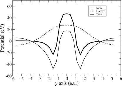
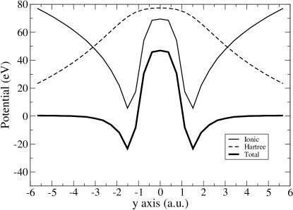
Figure 2: Calculated total and ionic and Hartree potentials for a 3D-periodic (top) and 1D-periodic (bottom) Si chain

.

In Fig. 2 (top) it is shown the ionic potential, the Hartree potential, and their sum for a Si atom in a parallelepiped supercell with side lengths of 2.5, 11, and 11 a.u. respectively in the $x$, $y$ and $z$ directions. No cutoff is used here. The ionic potential is roughly behaving like $\frac{1}{r}$ in the area not too close to the nucleus (where the pseudopotential takes over). The total potential, on the other hand, falls off rapidly to an almost constant value at around 4 a.u. from the nuclear position, by effect of the electron screening.

Fig. 2 (bottom) shows the results when the cutoff is applied (the radius of the cylinder is $R=5.5$ a.u. such that there is zero interaction between cells). The ionic potential now behaves like it is expected for a potential of a chain, i.e. diverges logarithmically, and is clearly different from the latter case. Nevertheless the sum of the ionic and Hartree potential is basically the same as for the 3D-periodic system.

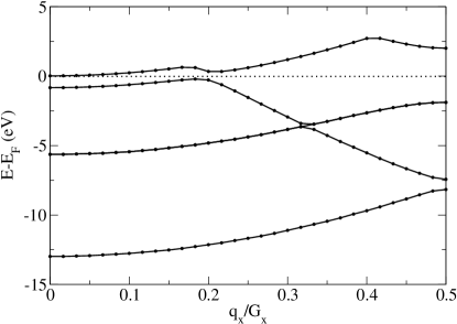
Figure 3: Si linear chain in a supercell size of 4.9x19x19 a.u.

In the static case the two band structure are then expected, and are found to be the same, confirming that, as far as static calculations are performed, the supercell approximation is good, provided that the supercell is large enough (see Fig. 3). In static calculations, then, the use of our cutoff only has the effect of allowing us to eventually use a smaller supercell, what provides clear computational savings. In the case of the Si-chain a full 3D calculation would need of a cell size of 38 a.u. whereas the cutoff calculation would give the same result with a cell size of 19 a.u. Of course, when more delocalized states are considered, like higher energy unoccupied states, larger differences are observed with respect to the supercell calculation.

In Fig. 4 a Na chain with lattice constant 7.5 a.u. is considered in a cell of 7.5x19x19 a.u., and the effect of the cutoff on the occupied and unoccupied stated is shown. As expected, the occupied states are not affected by the use of the cutoff, since the density of the system within the cutoff radius is unchanged, and the corresponding band is the same as it is found for an ordinary 3D supercell calculation with the same cell size. However there is a clear effect on the bands corresponding to unoccupied states, and the effect is larger the higher is the energy of the states. In fact the high energy states, and the states in the continuum are more delocalized, and therefore the effect of the boundary conditions is more sensible.

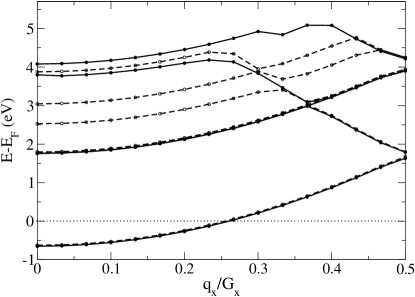
Figure 4: Effect of the cutoff in a Na linear chain in a supercell size of 7.5x19x19 a.u. The bands obtained with an ordinary supercell calculation with no cutoff (dashed line) are compared to the bands obtained applying the 1D cylindrical cutoff (solid line). As it is explained in the text, only the unoccupied levels are affected by the cutoff.

V.2 Static polarisability

After the successful analysis of the ground state properties with the cutoff scheme, we have applied the modified Coulomb potential to calculate the static polarisability of an infinite chain in the Random Phase Approximation (RPA). As a test case we have considered a chain made of hydrogen atoms, two atoms per cell at a distance of 2 a.u. The lattice parameter was 4.5 a.u. For this system we have also calculated excited state properties in many-body perturbation theory, in particular the quasiparticle gap in Hedin’s GW approximation GW and the optical absorption spectra in the Bethe-Salpeter frameworkOnida02 ; bse (see subsections below). All these calculations have been performed in the code SELF.self The polarisability for the monomer, i.e. a finite system, in the RPA approximation including local field effects is defined as

$$\alpha=-\lim_{{\bf q\rightarrow 0}}\frac{1}{q^{2}}\chi^{\phantom{0}}_{00}({\bf q})\frac{\Omega}{4\pi}.$$ (29)

where $\chi^{\phantom{0}}_{GG^{\prime}}(q)$ is the interacting polarisation function that is solution of the Dyson like equation

$$\chi^{\phantom{0}}_{GG^{\prime}}({\bf q})=\chi^{0}_{GG^{\prime}}({\bf q})+\sum_{G^{\prime\prime}}\chi^{0}_{GG^{\prime\prime}}({\bf q})v({\bf q+G^{\prime\prime}})\chi^{\phantom{0}}_{G^{\prime\prime}G^{\prime}}({\bf q}).$$ (30)

and $\chi^{0}$ is the non interacting polarisation function obtained by the Adler-Wiser expression.adler v(q+G) are the Fourier components of the Coulomb interaction. Note that the expression of $\alpha$ in Eq. 29 is also valid for calculations in finite systems, in the supercell approximation, and the dependence from the wave-vector $q$ is due to the representation in reciprocal space.

In the top panel of Fig. 5 we compare the values of the calculated polarisability $\alpha$ for different supercell sizes. $\alpha$ is calculated both using the bare Coulomb $v({\bf q+G})=\frac{4\pi}{|{\bf q+G}|^{2}}$ and the modified cutoff potential of Eq.(12) (the radius of the cutoff is always set to half the inter-chain distance). The lattice constant along the chain axis is kept fixed. Using the cutoff the static polarisability already converges to the asymptotic value with an inter-chain distance of 25 a.u., while without the cutoff the convergence is much slower, and the exact value is approximated to the same accuracy for much larger cell sizes (beyond the calculations shown in the top of Fig. 5).

We must stress that the treatment of the divergences in this case is different with respect to the case of the Hartree and ionic potential cancellation for ground-state calculations (i.e. charge neutrality). In fact, while in the calculation for the Hartree and ionic potential the diverging terms are simply dropped by virtue of the neutralising positive background, here the $h$-dependence in Eq. (25) can be removed only for the head component by virtue of the vanishing limit $lim_{{\bf q}\to 0}\chi^{0}_{00}({\bf q})=0$, while for the other $G_{x}=0$ components we have to resort to the expression of the finite cylindrical cutoff as in Eq.(25).

A finite version of the 1D cutoff has been recently applied to nanotube calculations.Spataru04 ; Spataru04b This cutoff was obtained by numerically truncating the Coulomb interaction along the axis of the nanotube, in addition to the radial truncation. Therefore the effective interaction is limited to a finite cylinder, whose size can be up to a hundred times the unit cell size, depending on the density of the k-point sampling along the axis.maxh The cutoff axial length has to be larger than the expected bound exciton length.

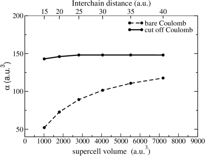
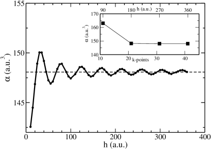
Figure 5: Top: Polarisability per unit cell of an $H_{2}$ chain in RPA approximation as a function of the supercell volume. The solid line joins the values obtained with the cutoff potential, while the dashed lines joins the values obtained with the bare Coulomb potential. The cutoff radius is 8.0 a.u. The inter-chain distance is indicated in the top axis. Bottom: Polarisability of the $H_{2}$ chain calculated with the finite cutoff potential of Ref.Spataru04b, . In abscissa different values of the cutoff length along the chain axis. The dashed straight line indicates the value obtained with the cutoff of Eq.(12).In the inset we show the convergence of the polarisability with respect to the k-points sampling along the chain axis obtained with the cutoff of Eq.(12). In the upper axis it is indicated the maximum allowed length $h$ for each k-point sampling used in the calculation of the $G_{x}=0$ components by Eq.(25).

In the bottom part of Fig.5 we compare the results obtained with our analytical cutoff (Eq. (12)) with its finite special case as proposed in Ref. Spataru04b, . We observe that the value of the static polarisability calculated with the finite cutoff oscillates around an asymptotic value, for increasing axial cutoff lengths. The asymptotic value exactly coincides with the value that is obtained with our cutoff. We stress that we also resort to the finite form of the cutoff only for the diverging of components of the potential, thus we note that there is a clear numerical advantage in using our expression, since the cutoff is analytical for all values except at $G_{x}=0$, and the corresponding quadrature has to be numerically evaluated for these points only. In the inset of the bottom part of Fig. 5 it is also shown the convergences of the polarisability obtained with our cutoff with respect to the k-points sampling. The sampling is unidimensional along the axial direction. Observe that the calculation using our cutoff is already converged for a sampling of 20 k-points. In the upper axis it is also indicated the corresponding maximum allowed value of the finite cutoff length in the axial direction that has been used to calculate the $G_{x}=0$ components.

Finite size effects turn out to be relevant also for many-body perturbation theory calculations. For the same test system (linear H₂-chain), in the next two subsections, we consider the performance of our cutoff potential for the calculation of the quasiparticle energies in GWGW approximation and in the absorption spectra in the Bethe-Salpeter framework.Onida02 ; bse

V.2.1 Quasiparticles in the GW approximation

In the GW approximation, the non-local energy-dependent electronic self-energy $\Sigma$ plays a role similar to that of the exchange-correlation potential of DFT. $\Sigma$ is approximated by the convolution of the one electron Green’s function and the dynamically screened Coulomb interaction $W$. We first calculate the ground state electronic properties using the DFT code ABINIT.abinit These calculation are performed in LDApz , and pseudopotentialstrouiller approximation. An energy cutoff of 30 hartree has been used to get converged results. The LDA eigenvalues and eigenfunctions are then used to construct the RPA screened Coulomb interaction $W$, and the GW self-energy. The inverse dielectric matrix $\epsilon^{-1}_{G,G^{\prime}}$ has been calculated using the plasmon-pole approximation plasmonpole and the quasiparticle energies have been calculated at the first order of perturbation theory in $\Sigma-V_{xc}$.Hybertsen Dividing the self-energy in an exchange $\Sigma_{x}$ and a correlation $\Sigma_{c}$ parts ($\langle\phi_{j}^{DFT}|\Sigma|\phi_{i}^{DFT}\rangle=\langle\phi_{j}^{DFT}|\Sigma_{x}|\phi_{i}^{DFT}\rangle+\langle\phi_{j}^{DFT}|\Sigma_{c}|\phi_{i}^{DFT}\rangle$), we get the following representation for the self-energy in a plane-waves basis set:

$$\langle n{\bf k}|\Sigma_{x}({\bf r_{1},r_{2}})|n^{\prime}{\bf k^{\prime}}\rangle=-\sum_{n_{1}}\int_{Bz}\frac{d^{3}{\bf q}}{(2\pi)^{3}}\sum_{G}v(\bf{q+G})\times\\ \times\rho^{\phantom{\star}}_{nn_{1}}({\bf q,G})\rho_{n^{\prime}n_{1}}^{\star}({\bf q,G})f_{n_{1}{\bf k_{1}}}$$ (31)

and

$$\langle n{\bf k}|\Sigma_{c}({\bf r_{1},r_{2}},\omega)|n^{\prime}{\bf k^{\prime}}\rangle=\frac{1}{2}\sum_{n_{1}}\int_{Bz}\frac{d^{3}{\bf q}}{(2\pi)^{3}}{\Bigg{\{}}\sum_{{\bf GG^{\prime}}}v(\bf{q+G^{\prime}})\\ \times\rho^{\phantom{\star}}_{nn_{1}}({\bf q,G})\rho_{n^{\prime}n_{1}}^{\star}({\bf q,G^{\prime}})\int\frac{d\omega^{\prime}}{2\pi}\epsilon^{-1}_{{\bf GG^{\prime}}}({\bf q},\omega^{\prime})\\ \times{\Big{[}}\frac{f_{n1({\bf k-q})}}{\omega-\omega^{\prime}-\epsilon^{LDA}_{n1({\bf k-q})}-i\delta}+\frac{1-f_{n1({\bf k-q})}}{\omega-\omega^{\prime}-\epsilon^{LDA}_{n1({\bf k-q})}+i\delta}\Big{]}{\Bigg{\}}}$$ (32)

where $\rho_{nn_{1}}({\bf q+G})=\langle n{\bf k}|e^{i({\bf q+G})\cdot{\bf r_{1}}}|n_{1}{\bf k_{1}}\rangle$ and the integral in the frequency domain in Eq.(32) has been analytically solved considering the dielectric matrix in the plasmon pole mode: ( $\epsilon^{-1}_{{\bf G,G^{\prime}}}(\omega)=\delta^{\phantom{-1}}_{\bf{G,G^{\prime}}}+\Omega^{\phantom{-1}}_{{\bf G,G^{\prime}}}/(\omega^{2}-\tilde{\omega}^{2}_{G,G^{\prime}})$).

In order to eliminate the spurious interaction between different supercells, leaving the bare Coulomb interaction unchanged along the chain direction, we just introduce the expression of Eq.(12) in the construction of $\Sigma_{x}$ and $\Sigma_{c}$, and also in the calculation of $\epsilon^{-1}_{GG^{\prime}}$. As we did for the calculation of the static polarisability, the divergences appearing in the components $(G_{x}=0)$ cannot be fully removed and for such components we resort to the finite version of the cutoff potential Eq.(25).

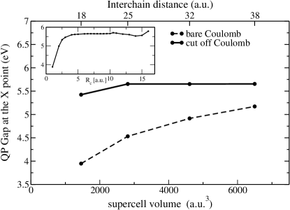
Figure 6: Convergence of the GW quasiparticle gap for the $H_{2}$ chain as a function of the cell size, using the bare Coulomb potential (dashed line) and the cutoff potential (solid line).In the inset the behaviour of the GW quasiparticle gap as a function of the value of the cutoff radius for a supercell with inter-chain distance of 32 a.u. is shown. The plateau obtained around a radius of 8 a.u. (i.e. one fourth of the supercell size) corresponds to the situation in which the radial images of chains no longer mutually interact, and the calculation is converged. Increasing the radius above approximately 12 a.u. the interaction is back and produces oscillations in the value of the gap.

In Fig. 6 the convergence of the quasiparticle gap at the $X$ point is calculated for different supercell sizes in the GW approximation. A cutoff radius of 8.0 a.u. has been used. When the cutoff potential is used, 60 k points in the axis direction has been necessary to get converged results. In the inset of Fig. 6 we show the behaviour of the quasiparticle gap in function of the cutoff radius. We observe that for $R_{c}>6$ a.u. a plateau is reached, and, for $R_{c}>12$ a.u., a small oscillation appears due to interaction between the tails of the charge density of the system with its image in the neighbour cell. Differently from the DFT-LDA, calculation for neutral systems, where the supercell approximation turns out to be good, as we have discussed above, we can see that the convergence of the GW quasiparticle correction turns out to be extremely slow with respect to the size of the supercell and huge supercells are needed in order to get converged results. This is due to the fact that in the GW calculation the addition of an electron (or a hole) to the system induces charge oscillation in the periodic images too. It is important to note that the slow convergence is caused by the correlation part of the self-energy (Eq.(32)), while the exchange part is rapidly convergent with respect to the cell size. The use of the cutoff Coulomb potential really improves drastically the convergence as it is evident from Fig.6. Notice that still at 38 a.u. inter-chain distance the GW gap is underestimated by about 0.5 eV. A similar trend (but with smaller variations) has been found by Onida et al. Onida95 , for a finite system (Sodium Tetramer) using the cutoff potential of Eq.(11). Clearly there is a strong dimensionality dependence of the self-energy correction. The non-monotonic behaviour versus dimensionality of the self-energy correction has also been pointed out in Ref. delerue, where the gap-correction was shown to have a strong component of the surface polarisation.

V.2.2 Exciton binding energy: Bethe-Salpeter equation

Starting from the quasiparticle energies we have calculated the optical absorption spectra including electron-hole interactions solving the Bethe-Salpeter equation bse . The basis set to describe the exciton state is composed by product states of the occupied and unoccupied LDA single particle states and the coupled electron-hole excited states $|S\rangle=\sum_{cv{\bf k}}A_{cv{\bf k}}a^{\dagger}_{c{\bf k}}a_{v{\bf k}}|0\rangle$, where $|0\rangle$ is the ground state of the system. $A_{cv{\bf k}}$ is the probability amplitude of finding an excited electron in the state $(c{\bf k})$ and a hole in $(v{\bf k})$, and it satisfies the equation

$$(\epsilon^{QP}_{c{\bf k}}-\epsilon^{QP}_{v{\bf k}})A_{vc{\bf k}}+\sum_{vc{\bf k},v^{\prime}c^{\prime}{\bf k^{\prime}}}K_{vc{\bf k},v^{\prime}c^{\prime}{\bf k^{\prime}}}A_{v^{\prime}c^{\prime}{\bf k^{\prime}}}=E_{S}A_{vc{\bf k}}$$ (33)

$E_{S}$ is the excitation energy of the state $|S\rangle$ and $K$ the interaction kernel that includes an unscreened exchange repulsive term $K^{Exch}$ and a screened electron-hole interaction $K^{dir}$ (direct term). In plane wave basis such terms read

$$K^{Exch}_{{vc{\bf k}\choose v^{\prime}c^{\prime}{\bf k^{\prime}}}}=\frac{2}{\Omega}\sum_{{\bf G\neq 0}}v({\bf G})\langle c{\bf k}|e^{i{\bf G\cdot r}}|v{\bf k}\rangle\langle v^{\prime}{\bf k^{\prime}}|e^{-i{\bf G^{\prime}\cdot r}}|c^{\prime}{\bf k^{\prime}}\rangle$$ (34)

$$K^{dir}_{{vc{\bf k}\choose v^{\prime}c^{\prime}{\bf k^{\prime}}}}= \frac{1}{\Omega}\sum_{{\bf G,G^{\prime}}}v({\bf q+G})\epsilon^{-1}_{{\bf GG^{\prime}}}({\bf q})\langle c{\bf k}|e^{i{\bf(q+G)\cdot r}}|c^{\prime}{\bf k^{\prime}}\rangle\times$$

$$\times\langle v^{\prime}{\bf k^{\prime}}|e^{-i{\bf(q+G^{\prime})\cdot r}}|v{\bf k}\rangle\delta_{\bf{q.k-k^{\prime}}}$$

The screened potential has been treated in static RPA approximation (dynamical effects in the screening have been neglected as it is usually done in present Bethe-Salpeter calculationsbse ). The quasiparticle energies entering in the diagonal part of the Hamiltonian in Eq. (33) are obtained applying a scissor operator to the LDA energies, because in the studied test case the main difference between the quasiparticle and LDA band structure consists of a rigid energy shift of energy bands. From the solution of the Bethe-Salpeter equation (Eq.33) it is possible to calculate the macroscopic dielectric function, in particular the imaginary part reads

$$\epsilon_{2}(\omega)=\frac{1}{\Omega}\frac{4\pi^{2}e^{2}}{\omega^{2}}\sum_{S}\Bigg{|}\sum_{vc{\bf k}}A^{S}_{vc{\bf k}}\langle v{\bf k}|\boldsymbol{\lambda}\cdot\boldsymbol{\nu}|c{\bf k}\rangle\Bigg{|}^{2}\delta(E_{S}-\hbar\omega)$$ (36)

where the summation runs over all the vertical excitations from the ground state $|0\rangle$ to the excited state $|S\rangle$, $E_{S}$ is the corresponding excitation energy, $\boldsymbol{\nu}$ is the velocity operator and $\boldsymbol{\lambda}$ is the polarisation vector. As in the case of GW calculation, in order to isolate the chain, we substitute the cutoff potential of Eq.(12) both in the exchange term Eq.(34) and in the direct term of the Bethe-Salpeter equation Eq.(LABEL:direct), as well as for the RPA dielectric matrix present in Eq.(LABEL:direct).

In the top part of Fig. 7 we show the calculated spectra for different cell sizes together with the non-interacting spectrum, and the spectrum obtained using the cutoff Coulomb potential for an inter-chain distance larger than 20 a.u. and cylindrical cutoff radius of 8 a.u. The scissor operator applied in this calculation is the same for all the volumes and correspond to the converged GW gap.

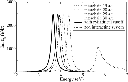
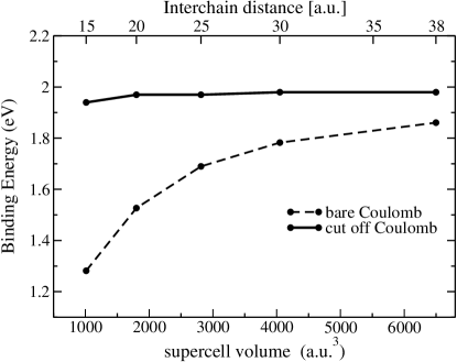
Figure 7: Top: Photo absorption cross section for different supercell volumes. In the legend the inter-chain distances corresponding to each volume are indicated. The intensity have been normalised to the volume of the supercell. The non-interacting absorption spectra and the spectra obtained with the cutoff potential are also included. Bottom: exciton binding energy vs supercell volume calculated using the cut off potential (solid line), and the bare Coulomb potential (dashed line).

As it is known, the electron-hole interaction modifies both the shape and the energy of the main absorption peak. This effect is related to the the slow evolution of the polarisability per $H_{2}$ unitdaniele . Furthermore, the present results clearly illustrate that the spectrum calculated without the cutoff slowly converges towards the exact result. This is highlighted in the bottom panel of Fig. 7 where we show the dependency of the exciton binding energy on the supercell volume, the binding energy being defined as the energy difference between the excitonic peak and the optical gap. We observe that the effect of the inter-chain interaction consists in reducing the binding energy with respect to its value in the isolated system. This value is slowly approached as the inter-chain distance increases, while, once the cutoff is applied to the Coulomb potential, the limit is reached as soon as the densities of the system and its periodical images do not interact. If we consider the convergence of the quasiparticle gap and of the binding energy with respect to the cell volume we notice that, if a cutoff is not used, the position of the absorption peak is controlled by the convergence of the Bethe-Salpeter equation solution, which, in turn, depends on the (slower) convergence of the GW energies. It is clear from Fig. 6 that the use of the cutoff allows us to considerably speed up this bottleneck.

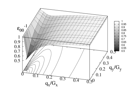
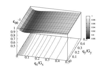
Figure 8: Values of $\epsilon^{-1}_{00}(q_{x},q_{y})$ in the $q_{z}=0$ plane for the $H_{2}$ chain with an inter-chain distance of 25 a.u., using the bare Coulomb (top) and the cutoff potential (bottom). The axis of the chain is along the x direction

The use of our cutoff also has an important effect on the Brillouin zone sampling. In Fig. 8 we show the value of $\epsilon^{-1}_{00}(q_{x},q_{y})$ in the $q_{z}=0$ plane for a supercell corresponding to an inter-chain distance of 25 a.u. When the cutoff potential is used (bottom panel) the screening is smaller, compared to the case of the bare potential (top panel). Looking at the direction perpendicular to the chain (the chain axis is along the $x$ direction) we see that the dielectric matrix is approximately constant, and this fact allows us to sample the Brillouin zone only in the direction of the chain axis. For both the GW and Bethe-Salpeter calculations a three dimensional sampling of the Brillouin zone is needed to get converged results when no cutoff is used, while a simple one-dimensional sampling can be adopted when the interaction is cutoff.

VI Conclusions

An infinite system is an artifact that allows us to exploit the powerful symmetry properties of an ideal system to approximate the properties of a finite one that is too large to be simulated at once. In order to use the valuable supercell approximation for systems that are periodic in less than three dimensions some cutoff technique is required. The technique presented here provides a recipe to build the supercell, and a truncated Coulomb potential in Fourier space in such a way that the interactions to all the undesired images of the system are cancelled. This technique is exact for the given supercell sizes, and can be in most cases well approximated using supercells whose length is the double of the system size in the non-periodic dimensions. The method is very easily implemented in all available codes that use the supercell scheme, and is independent on the adopted basis set. We have tested it both in a real space code for LDA band-structure calculation of an atomic chain, and a plane wave code, for the static polarisability in RPA approximation, GW quasiparticle correction, and photo-absorption spectra in the Bethe-Salpeter scheme, showing that the convergence with respect the vacuum needed to isolate the system from its images is greatly enhanced, and the sampling of the Brillouin zone is heavily reduced, being only necessary along the periodic directions of the system.

- (1) M. L. Cohen, Solid Stat. Commun. 92, 45 (1994); Phys. Scri. 1, 5 (1982). J. Ihm, A. Zunger and M. L. Cohen, J. Phys. C 12, 4409 (1979). W. E. Pickett, Comput. Phys. Rep. 9, 115 (1989); M. C. Payne, M. P. Teter, D. C. Allan, T. A. Arias and . D. Joannopoulos, Rev. Mod. Phys. 64, 1045 (1992).
- (2) M. Frigo, S. G. Johnson, Proc. IEEE Int. Conf. Acoust. Speech, Signal Processing, ICASSP’98, 3, 1381 (1998)
- (3) J. E. Lebowitz, E. H. Lieb, Phys. Rev. Lett. 22 631 (1969)
- (4) See for example: A.P. Alivisatos, Science 271, 933 (1996); Carbon Nanotubes: Synthesis, Structure, Properties, and Applications, M.S. Dresselhaus, G. Dresselhaus, and Ph. Avouris (Editors), Springer Verlag (2001); Encyclopedia of Nanoscience and Nanotechnology and Handbook of Nanostructured Biomaterials and Their Applications in Nanobiotechnology, H. S. Nalwa (editor), American Scientific Publishers (2005); Quantum Computing and Quantum Communication, G. Burkard, H-A. Engel, and D. Loss, http://theorie5.physik.unibas.ch/qcomp/qcomp.html
- (5) The maximum value of the size of the cutoff axial length both in Ref. Spataru04b, and in Eq. (25) is , where is the spacing of the k-point grid in the direction of the cylinder axis.
- (6) L. Hedin, Phys. Rev. 139, 796 (1965); L. Hedin and S. Lundqvist, Solid State Phys 23, 1 (1969); F. Aryasetiawan and O. Gunnarson, Rep. Prog. Phys. 61, 237 (1998); W. G. Aulbur, L. Jönsson and J.W. Wilkins, Solid State Physics 54, 1 (1999).
- (7) G. Onida, L. Reining, A. Rubio, Rev. Mod. Phys. 74, 601 (2002), and references therein.
- (8) Sottile, F. Bruneval, A. G. Marinopoulos, L. Dash, S. Botti, V. Olevano, N. Vast, A. Rubio and L. Reining, Int. J. Quantum Chem. 112, 684 (2005).
- (9) B. Wood, W. M. C. Foulkes, M. D. Towler, and N.D. Drummond, J. Phys.: Condens. Matter 16, 891 (2004)
- (10) G. Makov, M.C. Payne, Phys Rev. B 51, 4014 (1995)
- (11) S. W. DeLeeuw, J. W. Perram, E. R. Smith, Proc. R. Soc. Lond. A 373, 27 (1980)
- (12) P. P. Ewald, Ann. Phys. 64, 253 (1921)
- (13) E. Spohr, J. Chem. Phys. 107 6342 (1994)
- (14) I. Yeh, M. Berkowitz, J. Chem. Phys. 111, 3155 (1999)
- (15) G. J. Martyna, M. E. Tuckerman, J. Chem. Phys 110, 2810 (1999)
- (16) A. Bródka, Mol. Phys. B 61, 3177 (2003)
- (17) D. M. Heyes, M. Barber, J. H. R. Clarke, J. Chem. Soc. Faraday Trans II 73, 1485 (1977)
- (18) A. Grzybowski, E. Gwóźdź, A. Bródka, Phys. Rev. B 61, 6706 (2000)
- (19) P. Mináry, M. E. Tuckerman, K. A. Pihakari, and G. J. Martyna J. Chem. Phys. 116, 5351 (2002)
- (20) P. Mináry, J. A. Morrone, D. A. Yarne, M. E. Tuckerman, and G. J. Martyna, J. Chem. Phys. 121, 11949 (2004)
- (21) P.A. Schultz, Phys. Rev. B 60, (1999) 1551
- (22) R. W. Hockney and J. W. Eastwood, Computer Simulations Using Particles, Mc-Graw Hill, New York, 1981
- (23) M. R. Jarvis, I. D. White, R. W. Godby, M. C. Payne, Phys. Rev. B 56, 14972 (1997)
- (24) L. Greengard, The rapid evaluation of potential fields in particle systems, (MIT Cambridge, MA, 1987)
- (25) A. Castro, A. Rubio, M. J. Stott, Can. J. Phys. 81, 1 (2003)
- (26) K. N. Kudin, G. E Scuseria, J. chem. Phys. 121, 2886 (2004).
- (27) M. A. L. Marques, A. Castro, G. F. Bertsch, A. Rubio, Comput. Phys. Commun. 151, 60 (2003)
- (28) G. Onida, L. Reining, R. W. Godby, R. Del Sole and W. Andreoni, Phys. Rev. Lett. 75, 818 (1995).
- (29) J. D. Jackson, Classical Electrodynamics, Wiley (1999)
- (30) C. Spataru, S. Ismail-Beigi, L. X. Benedict, S. G. Louie Applied Physics A 78, 1129 (2004)
- (31) I. S. Gradshteyn, M. Rhysik, Tables of Integrals, Series and Products (Academic, New York, 1980)
- (32) http://people.roma2.infn.it/marini/self/
- (33) http://www.abinit.org
- (34) N. Troullier, J. L. Martins, Phys. Rev. B 43, 1993 (1991)
- (35) J. P. Perdew and A. Zunger, Phys. Rev. B 23, 5048 (1981)
- (36) S.Albrecht, L. Reining, R. Del Sole and G. Onida, Phys. Rev. Lett. 80, 4510 (1998); L. X. Benedict, E.L. Shirley, R. B. Bohn, ibid. 80, 4514 (1998); M. Rohlfing and S.G. Louie, ibid. 81 , 2312 (1998); Pys. Rev. B 62, 4927 (2000)
- (37) S. L. Adler, Phys. Rev. 126, 413 (1962); N. Wiser, Phys. Rev. 129, 62 (1963)
- (38) C.D. Spataru, S. Ismail-Beigi, L. X. Benedict, S. G. Louie Phys. Rev. Lett. 92, 077402 (2004)
- (39) R. W. Godby, R. J. Needs, Phys. Rev. Lett. 62, 1169 (1989). To get converged inverse dielectric matrix we have used unoccupied bands up to 28 eV in the electron-hole energies, and a number of vectors until in the inversion of the matrix.
- (40) M. S. Hybertsen and S. G. Louie, Phys. Rev. Lett. 55, 1418 (1985); R.W. Godby, M. Schluter, L. J. Sham, Phys. Rev. B 37, 10159 (1988)
- (41) C. Delerue, G. Allan, M. Lannoo, Phys. Rev. Lett. 90, 076803 (2003)
- (42) D. Varsano, A. Marini, A. Rubio (work in progress)