Game Theory and Topological Phase Transition

Abstract

Phase transition is a war game. It widely exists in different kinds of complex system beyond physics. Where there is revolution, there is phase transition. The renormalization group transformation, which was proved to be a powerful tool to study the critical phenomena, is actually a game process. The phase boundary between the old phase and new phase is the outcome of many rounds of negotiation between the old force and new force. The order of phase transition is determined by the cutoff of renormalization group transformation. This definition unified Ehrenfest’s definition of phase transition in thermodynamic physics. If the strategy manifold has nontrivial topology, the topological relation would put a constrain on the surviving strategies, the transition occurred under this constrain may be called a topological one. If the strategy manifold is open and noncompact, phase transition is simply a game process, there is no table for topology. An universal phase coexistence equation is found, it sits at the Nash equilibrium point. Inspired by the fractal space structure demonstrated by renormalization group theory, a conjecture is proposed that the universal scaling law of a general phase transition in a complex system comes from the coexistence equation around Nash equilibrium point. Game theory also provide us new understanding to pairing mechanism and entanglement in many body physics.

I Introduction

When physicists encounter millions of interacting molecules or atoms, they can not control the trajectory or momentum of each individual particles, so they study the macroscopic states at different temperature or other physical parameter. In most cases, there would be some significant change of the macroscopic states at certain value of parameters, they call it a phase transition. Phase transition are common phenomena in all branches of physics. People’s interest in phase transition can trace back to thousands of years ago. A recent example is the superfluid-Mott-insulator phase transition occurred in a gas of ultracold atoms in optical latticegreiner .

Statistic mechanics were developed to provide a theoretical description of phase transition. The occurrence of phase transition is related to the singularity of statistical functions in the thermodynamic limit(see Ref. stanley for review). However statistical mechanics is not powerful enough to predict all different kind of phase transition. For classical Hamiltonian systems, the hypothesis connecting phase transitions to the change of configuration space topology was proposed recent years(see Ref. kastner and references therein for review). Topological order also rise in quantum systems (see Ref. wen for review), such as the fractional quantum Hall system. Different fractional quantum Hall effect states all have the same symmetry, that is beyond the Landau s symmetry breaking theory. The topological order in quantum system is related to degenerate ground states, quasiparticle statistics, edge states, or momentum topologyvolovik , et al. These topological order theory told us many interesting phenomena in some special models and special systems. However it is still far from providing us an universal explanation to phase transition occurred in all different branches of physics, much less in other complex system beyond physics.

Generally people believed that it is the thermal fluctuation that drives the transition from one phase to another in classical phase transition. As temperature is lowered, the thermal fluctuations are suppressed. The quantum fluctuation began to play a vital role in quantum phase transition. Unfortunately this kind of argument does not hold in many quantum system. More over, some physicist believed that phase transition is due to the competition between two competing orders in a physical system, but people can always propose some anomalous examples which can not be explained by two competing orders.

The occurrence mechanism of phase transitions is still not clear in countless systems. Similar critical phenomena arose in a broad physical and social systems. Many unrelated models covering physics, chemistry, biology present similar scaling laws. Anyone who saw this can not help asking why. Is there a ’theory of everything’ that can give us an universal explanation? Such a theory sounds like superstring theory.

What I am trying to do in this paper is not to establish the superstring theory of phase transition, but to present an universal theoretical explanation to phase transition occurred in different systems based on renormalization group theory and game theory, and beyond the two, such as topology, quantum field theory.

The first step is to break the envelop of physics and extend the concept of phase transition from physical system to complex system including chemistry system, biological system, social system, economic system, et al. Phase transition is a sudden jumping from one stable state to another. A two player game always has two stable states, the winning state and losing state. Thus we can define phase transition as a war game. If we check the war game carefully, one would see it has all the the same phenomena as phase transition occurred in physical system. War is a conflict between millions of soldiers who are armed and well organized. The butterfly effect is a basic character of war going on. The final destiny of the fighter is determined by some minor accidental event. When the two groups with equivalent force are fighting against each other but keeping at a draw state, if any one of them is reinforced a little, he will win the war in a few seconds. This is a phase transition.

So we can take phase transition as a war game, the strategies of the players extended the strategy base manifold. When we are studying the state evolution of the game corresponding to different strategy, the topology of the strategy base manifold comes in. The phase transition is a war game between new phase and old phase, each of them is governed by a kind of dominant interaction(it may has many minor affiliated companions). It will be shown in the main tex of this paper, the surviving strategy of the two phases carry opposite winding number, the sum of these winding numbers is a topological number on the strategy base manifold. After the winding number are annihilated by pairs, the last one winding number around the last surviving strategy is decided by the topological number, this also decided who will be the winner between the old phase and new phase. It is in this sense, we call it a topological phase transition. In fact, phase transition is always related to the topology of the strategy base manifold when the strategy base manifold is compact. In some cases, the base manifold is open and noncompact , there is no need to consider the effect of topological constrain. In fact, the compact strategy manifold like a finite region confined by fencing, it put some constrains on the way we choose strategy. There is singular point we can never eliminated smoothly in strategy space, that is the fundamental origin of topological phase transition.

The paper is organized as follows:

In section 2, the most general conception of phase transition in complex system is defined.

In section 3, we established the game theory of renormalization group transformation, and find the general solution of renormalization group transformation equations. The fundament classification of phase transition through symmetry losing is presented.

In section 4, topological current theory of phase transition is established, this theory spontaneously produced an universal equation of phase coexistence. A conjecture on the universal scaling law is proposed base on a topological hypothesis in fractal strategy space of game theory. Further more, we established the evolution equation of phases and the quantum phase coexistence equation.

In section 5, we developed the quantum statistics of many player game, and proposed a conjecture to find the fixed point of a many player game using quantum density matrix. More over, a new quantity to measure the entanglement of quantum states in a game is found. The single direction of renormalization group follows the second thermodynamic law, the renormalization flows to increase the entropy as well as the quantum entanglement. More over, the coexistence state of multi-player game is discussed.

In section 6, we developed the game theory of phase transition in classical many body system as well as quantum many body system. A new holographic topological quantity to characterize momentum space is proposed. We studied the quantum many body theory of war game and gave a new pairing mechanism base on prisoner dilemma.

The last section is devoted to a brief summary and outlook.

II Phase transition and war game

II.1 Phases of complex system

A complex system consists of many different elements that are connected or related, it appears like a black box to us. One can obtain the information within the complex system by its responses to external perturbation. These responses and perturbations are macroscopic variables. Different stable phases of complex system are characterized and distinguished by these observables.

For most condensed matter physicists, a liter of water is a complex system, since it is hardly possible to find exact analytical solution for the motion of $10^{27}$ $H_{2}O$ molecules. We can characterize its different phases by observing its chemical composition and physical properties, such as volume, pressure, temperature, density, crystal structure, index of refraction, chemical potential, and so forth. One of the main task of physicist is to find the relations among these macroscopic variables via presumably well known microscopic interactions between particles.

A stable phase has self-restoring ability when it is disturbed from equilibrium states. During a relative long life time, the chemical makeup does not decompose, and the physical properties keep a good manner. If we know the position and momentum of every particles in a dynamic system at a given time, the evolution of an integral system is exactly predictable. Unfortunately, there is few integrable many body system. The position and momentum of particles can not be exactly measured at the same time due to the Heisenberg uncertainty principal. So we define the state vector of a stable phase by the complete set of observables.

Let $\vec{x}$ be $n$ independent states of a complex system. For a physical system consists of $N$ interacting particles, the components of an arbitrary vector $\vec{x}_{i}$ are consists of $3N$ position coordinates $q_{1},q_{1},...,q_{3N}$, $3N$ momentum coordinates $p_{1},p_{1},...,p_{3N}$, and a vector of other physical parameters $\vec{\gamma}$, such as temperature $\gamma_{1}=T$, pressure $\gamma_{2}=P$, particle density $\gamma_{3}=N$, volume $\gamma_{4}=V$, chemical potential $\gamma_{5}=\mu$,$\cdots$, conductivity $\gamma_{j}=\sigma$, susceptibility $\gamma_{k}=\chi$, and so on. Here the state vector $\vec{x}=(\vec{q},\vec{p})$ is a much more general conception than that of statistical physics. It indicates the information inside the black box of any complex system.

The response of the complex system are induced by external input vector $\vec{\gamma}$. For physicist, $\gamma_{i}$ represents those familiar external applied magnetic field, electric field, pressure, neutrino current, electric current, detecting laser beams, heaters, and so forth. For chemist or biologist, the input vector represents something like enzymes, chemical accelerator.

Not all the components of the state vector are observable under perturbation. The output vector $\vec{y}$ represents those observables that people can definitely detected in laboratory. The output is strongly depend on what people want to study. For example, there are circulatory systems, nervous systems and digestive systems within human body. If we are studying the human population, there is no need to take into account of these subsystems; one only counts the people, the output vector covers the number of people, distribution of people, etc. If the subject is about flu’s spread, it may be best to discuss the immune subsystem.

For a general dynamic system

$$\frac{d\vec{x}_{in}}{dt}=F_{in}(\vec{x},\vec{\gamma}),\;\;\;\;\;\;\;\vec{O}_{ut}=F_{out}(\vec{x},\vec{\gamma}),$$ (1)

the output vector is not always differentiable for all degrees of differentiation on the whole range of the parameter space $M(\vec{x},\vec{\gamma})$. There exist critical points $(\vec{x}^{\ast},\vec{\gamma}^{\ast})$ at which the $C^{k}$ output functions blow up. The whole input space is divided into separated blocks by these critical points,

$$M^{0}(\vec{r})=\{({r}_{1}^{\ast},{r}_{2}^{\ast})\cup({r}_{2}^{\ast},{r}_{3}^{\ast})\cdots\cup({r}_{n}^{\ast},{r}_{n}^{\ast})\},$$ (2)

here we denote $({r}:=(\vec{x},\vec{\gamma}))$. The stable phase are defined in these discrete blocks. The output functions present very good behavior within the blocks but diverge at the very boundary. These boundaries are where the phase transition occurs.

This general mathematical definition of phases for complex system applies for many different fields. The most familiar Ehrenfest’s definitionehrenfest of phase transition in thermodynamics is a good exemplar. The output vector is only a function—free energy. The input vectors are thermodynamic quantities, temperature $T$ and pressures $P$. For the zeroth order stable phase the free energy of the two phases $F(T,P)$ is $C^{\infty}$ in the whole input space $(T,P)\in[-\infty,+\infty]$. For the first order phase transition, the free energy $F(T,P)$ is continuous in the region $T\in[T_{i},T_{f}],P\in[P_{i},P_{f}]$, but the first order derivative is not continuous,

$$\frac{{\partial}F_{A}}{{\partial}T}\neq\frac{{\partial}F_{B}}{{\partial}T},\;\;\frac{{\partial}F_{A}}{{\partial}P}\neq\frac{{\partial}F_{B}}{{\partial}P},$$

$$T_{A}\in(T_{i},T_{c}),T_{B}\in(T_{c},T_{f}),$$

$$P_{A}\in(P_{i},P_{c}),P_{B}\in(P_{c},P_{f}).$$ (3)

The first order stable phase blocks are divided into smaller blocks by the second order phase transition.

The phase transition of complex system may be defined from the divergence of the $C^{k}$ output functions. They could be any observable functions. For mathematician, a stable phase is marked by a $C^{k}$ function in the discrete blocks on the input vector space. The critical point is the phase boundary between the separated blocks.

II.2 Phase transition

Figure 1: The whole phase diagram is split into discrete domains. The stable phase exist in the inner region. The domains wall is the phase coexistence region. In each domain, there is a dominant interaction which is the king ruling over the other weaker interaction. There is a war going on at the phase coexistence boundary. When we tune the physical parameters, we are helping a certain interaction to fight against the others, this certain phase would grow stronger and stronger, it will finally unified the whole phase diagram.

The stable output states of a dynamic complex system are confined in different domains in the whole input state vector space. As the input vector changes within a domain, the system is in a stable state, it represents a kind of physical order. When the input vector jumps from one domain to another, the system jumps from one stable phase to another. The domain wall is the exact phase boundary at which the old phase becomes unstable and decays, but the new phase comes into being and finally leads to new stable order. Phase transition occurs everywhere in nature. Every phase transition indicates a revolution induced by the interaction between the systems and their environment. the fittest states of the old domain is replaced by the fittest states of the new domain.

The lifeless nature world is much more intellectual than most physicists thought. What physicist measures in experiment is always the observable in equilibrium. Quantum theory tell us the energy levels of molecules and atoms are discrete and quantized, we can calculate the transitions probability between those levels involving the absorption or emission of photons. But we don’t know how and why that occurs. In principal, the non-equilibrium process of many particle system follows the same rules that govern the living systems, such as ants society, honeybees group, traffic system, etc.

If we focus on the behavior of particles before they reach equilibrium, one would doubt that electrons are possibly intelligent particles. One simple example is two resistors connected in parallel in electric circuit. As all knew, the current is proportional to the inverse of resistivity in subways. In the beginning, the electron moves together in the main path. When they reach the bifurcation point, they split into two subways. Less current in the strong resistive way, and larger current in the less resistive one. Like the cars in traffic, if all the electrons choose the less resistive way, they block each other until it becomes more resistive than the other subway. Then some electrons withdraw and transferred to the other way. There is no traffic jam in electric current network, because the cars are everywhere under the control of a global electric field.

The non-equilibrium dynamic process shows up in the vicinity of critical point, at which a small quantitative change of a parameter would results in a qualitative change of the global behavior of a complex system. Biological systems that adapt to their environment thrive, those that fail to evolve fade away. The environment are external input of the biological system. A stable phase of a biological system only exist in a finite region of environment parameters, so does a lifeless physical system. The stable phase of a collection of $H_{2}O$ molecules is water between 0^∘C$\sim$100^∘C, below 0^∘C(273 K) is ice crystal, and it becomes gas above 100^∘C.

Like any living creatures in nature, a lifeless physical system of interacting $H_{2}O$ molecules evolutes following the rule— ”survival of the fittest”. They took different collective structures according to different pressure, temperature, impurity, radiation, gravitation field, electric field, magnetic field, density, etc. The stablest phase at certain range of the parameter space survives as the fittest structure, the other phases in this domain fade away. Out of this special domain, the molecules have to reorganize their collective motion pattern in order to fit the new environment. When the new phase is born, the old phase dies.

The phase transition most scientists observed in physics, chemistry, biology, complex network, economics, $\cdots$ is a revolution. Phase transition is a war between the force of old phase and the force of new phase. The fundamental particles are millions of armed soldiers. They are divided into different large-scale armed groups who are fighting with one another. There is always a critical region in which the fighters bet their bottom dollar on one war, the winners take everything, the losers get nothing. This critical point is the phase boundary. Sometimes, the turning point is not so definite that it broadens into a finite region, this indicates a crossover transition.

III Renormalization group theory and game theory

III.1 Game theory and Renormalization group

Wilson’s renormalization group theory provides a fundamental non-perturbative approach to quantum critical phenomenawilson . One basic character of quantum many body system is that the microscopic particles are not distinguishable. Army is the best social system for simulating collective behaviors of quantum many particles in physics. Usually the soldiers are identical particles in the eyes of a general, but are distinguishable particles for a sergeant. The hierarchy structure of army plays the same role as quantum numbers in physics. The statistics of particles is scale dependent. One example is two column of dipolar Bosonic atoms obeying anyonic statistics due to the long range interaction. There are other biology system which similar to human society, such as ant group, honeybee group, we mainly take the army as a basic example to demonstrate renormalizattion group theory.

In Kadanoff constructionkadanoff , a certain number of neighboring particles are grouped into one cell which act as new elementary particles of the renormalized Hamiltonian. At critical point, the Hamiltonian is identical to the original Hamiltonian. For an army, this coarse-graining procedure naturally take place. An army has a hierarchical structure, the units of different size include a collection of lower rank of subordination particles. 100 men are group into a company, each company acts like one particle at higher rank marked by a captain. Every 10 companies form a regiment, the regime particle may be named after by colonel. This coarse-graining procedure take finite steps from brigade to division, to corps, and finally to an army.

In fact, the coarse-graining procedure is a simplification of army at war. In the microscopic level, it is the soldiers who are fighting with each other. Since they do not hate each other personally, they behave as indistinguishable identical particles, and fight as a whole. Renormalization theory simplifies the war between millions of soldiers to a war between thousands of companies, to a war between hundreds of regiments, finally to the war between two army. It is the war between two generals, it is also the war between hundred of colonels as well as captains.

The mean field theory view the war as a fight between two full generals dressed up by millions of soldiers. This is correct in most cases, but it is not always accurate, for the general’s strategy is carried out by hundreds of colonels and captains instead of the elementary soldiers. At the critical point, the correlation between the members of an army extends to its maximal value. As the butterfly effect says, the battle may be lost due to a nail which fail to fix the shoes of the horse. For want of the horse, a rider is lost. The lost of one rider may directly leads to the loss of a battle.

The renormalization group starts from the most fundamental particles of the army: soldiers. The first order renormalization is to reduce the interaction between millions of soldiers to hundred of captains which are dressed up by soldiers. The second order renormalization procedure is to identify effectively the captains belonging to one regiment with one colonel. This particle-blocking process may continue, and finally end up with full generals.

This explanation of renormalization group theory from war between armies is not merely a parable. There is a rigorous mathematical correspondence between the game theory of war and renormalization group theory. Let’s take the two-dimensional Ising model on triangle lattice as one example. The soldiers are spins $\sigma_{i}$, the battle field is the triangular lattice, the Hamiltonian of this game reads

$$H=\gamma_{1}\sum^{N}_{<ij>}\sigma_{i}\sigma_{j}+\gamma_{2}\sum^{N}_{i}\sigma_{i},\;\;\;(\sigma_{i}=\pm 1).$$ (4)

$\gamma_{1}=J/k_{B}T$ denotes the interaction between the nearest neighbor spins. $\gamma_{2}=\mu{B}/k_{B}T$ is the effective external applied magnetic field. This model may be treated as $N$-players game, the $N$ spins are $N$ players, each of them has two strategy $\pm 1$. The Hamiltonian is the payoff function. The players take different strategy to minimize the energy function. Another different modelling of this Ising model by game theory is to take it as a two-player game. We christen the two players ${\gamma}_{1}$ and ${\gamma}_{2}$. ${\gamma}_{1}$’s task is to choose a strategy $|{\gamma}_{1}\rangle$ in its strategy space $\{{\gamma}_{1}\}$ to control the interaction between neighboring soldiers, so that they act following his orders. ${\gamma}_{1}$ governs the soldiers by either ferromagnetic interaction or anti-ferromagnetic interaction. ${\gamma}_{2}$ commands the spin soldiers to keep strictly in the direction of external magnetic field. ${\gamma}_{1}$ and ${\gamma}_{2}$ choose different strategies to win this game.

A decision rule for ${\gamma}_{1}$ is a operator $\hat{f}_{{\gamma}_{1}}:\{{\gamma}_{2}\}\Rightarrow\{{\gamma}_{1}\}$, it associates each strategy $|{\gamma}_{2}\rangle{\in}\{{\gamma}_{2}\}$ of ${\gamma}_{2}$ with the strategies $|{\gamma}_{1}\rangle{\in}\hat{f}_{{\gamma}_{1}}|{\gamma}_{2}\rangle$, which may be played by ${\gamma}_{1}$ when he knows that ${\gamma}_{2}$ is playing $|{\gamma}_{2}\rangle$. Similarly, the decision rule for $|{\gamma}_{2}\rangle$ is a map $\hat{f}_{|{\gamma}_{2}\rangle}$ from $\{{\gamma}_{1}\}$ to $\{{\gamma}_{2}\}$. When a pair of strategies $(|\bar{\gamma}_{1}\rangle,|\bar{\gamma}_{2}\rangle)$ satisfies

$$|\bar{\gamma}_{1}\rangle{\in}\hat{f}_{{\gamma}_{1}}|\bar{\gamma}_{2}\rangle,\;\;\;|\bar{\gamma}_{2}\rangle{\in}\hat{f}_{{\gamma}_{2}}|\bar{\gamma}_{1}\rangle,$$ (5)

they form a consistent pair of strategies. The set of consistent pair may be empty or very large or it may reduce to a small number of bi-strategies. The problem of finding consistent strategy pairs is so-called fixed-point problem. We may construct a consistent map of the strategy pair,

$$\forall(|{\gamma}_{1}\rangle,|{\gamma}_{2}\rangle)\in{\{{\gamma}_{1}\}}\times{\{{{\gamma}_{2}}\}},\;\;\;\hat{f}(|{\gamma}_{1}\rangle,|{\gamma}_{2}\rangle):=\hat{f}_{{\gamma}_{1}}\times{\hat{f}_{{\gamma}_{2}}},$$ (6)

such that

$$\hat{f}_{AB}|{\gamma}_{1}\rangle=\hat{f}_{{\gamma}_{1}}{\hat{f}_{{\gamma}_{2}}}|{\gamma}_{1}\rangle=|{\gamma}^{\prime}_{1}\rangle\in{\{{\gamma}_{1}\}},\;\;\;$$ (7)

$$\hat{f}_{BA}|{\gamma}_{2}\rangle=\hat{f}_{{\gamma}_{2}}{\hat{f}_{{\gamma}_{1}}}|{\gamma}_{2}\rangle=|{\gamma}^{\prime}_{2}\rangle\in{\{{\gamma}_{2}\}}.$$ (8)

Then a consistent pair is explicitly written in the form,

$$\left(\begin{array}[]{c}|\bar{\gamma}_{1}\rangle\\ |\bar{\gamma}_{2}\rangle\\ \end{array}\right)=\left(\begin{array}[]{cc}0&\hat{f}_{{\gamma}_{1}}\\ \hat{f}_{{\gamma}_{2}}&0\\ \end{array}\right)\left(\begin{array}[]{c}|\bar{\gamma}_{1}\rangle\\ |\bar{\gamma}_{2}\rangle\\ \end{array}\right).$$ (9)

This decision rule matrix of the two players is just the renormalization group transformation matrix

$$\hat{U}=\left(\begin{array}[]{cc}0&\hat{f}_{{\gamma}_{1}}\\ \hat{f}_{{\gamma}_{2}}&0\\ \end{array}\right)$$ (10)

which can be deduced from the decimation procedure of renormalization group transformation. The players may play many steps to reach an agrement. Each time we group the spins in a sum by Kadanoff blocks, the original degree of freedom is decimated into the fewer degree of freedom. Every block is now a new giant elementary particle whose spin is determined by the majority rule. The Kadanoff-blocking process is actually a game process. After the first step of Kadanoff-blocking, the two player accomplished the first round of game, and their possible strategy space is reduced to a smaller one due to the information they get from the first round game.

The rescaled Hamiltonian is of the same form as the original one,

$$H^{\prime}=\gamma^{\prime}_{1}\sum^{N^{\prime}/2}_{<ij>}\sigma^{\prime}_{i}\sigma^{\prime}_{j}+\gamma^{\prime}_{2}\sum^{N^{\prime}}_{i}\sigma^{\prime}_{i}.$$ (11)

The new parameters represent the new strategy of the two players for the second round of the game, they follow the renormalization group transformation,

$$\gamma^{\prime}_{1}=\gamma^{\prime}_{1}(\gamma_{1},\gamma_{2}),\;\;\;\gamma^{\prime}_{2}=\gamma^{\prime}_{2}(\gamma_{1},\gamma_{2}).$$ (12)

We denote the strategy space of the two player as $K=\{|\gamma_{1}\rangle,|\gamma_{2}\rangle\}$, the strategy vector of the two players is

$$|\gamma\rangle=\left(\begin{array}[]{c}|\gamma_{1}\rangle\\ |\gamma_{2}\rangle\\ \end{array}\right).$$ (13)

The game operator is a map from the strategy space to itself,

$$\hat{U}:\;|\gamma\rangle\in{K}\rightarrow|\gamma^{\prime}\rangle\in{K}.$$ (14)

This game operator is equivalent to the renormalization group transformation. Applying Brouwer’s fixed point theorem, we know if the the strategy space is convex compact subsets of finite dimensional vector space, there is at least one pair of consistent strategy which satisfies

$$|\bar{\gamma}\rangle=\hat{U}|\bar{\gamma}\rangle.$$ (15)

$|\bar{\gamma}\rangle$ is the brouwer fixed point, or Nash equilibrium point. This fixed is the saddle point of physical observables on the manifold expanded by $(\gamma_{1},\gamma_{2})$.

This game operator for the two dimensional Ising model may be derived from the recursion relation the semigroup transformation,

$$\vec{\gamma}^{\prime}=\hat{{U}}_{L}\vec{\gamma},$$ (16)

$$\vec{\gamma}^{\prime}=(\gamma^{\prime}_{1},\gamma^{\prime}_{2}),\;\vec{\gamma}=(\gamma_{1},\gamma_{2}).$$ (17)

here $L$ is rescaling factor of Kadanoff-blocking. We calculate a statistical physical observable, such as free energy

$$F=-\frac{1}{\beta}ln\;Z,\;\;\;Z=Tr\;e^{-\beta{H(\gamma_{i}(t))}},$$ (18)

using the rescaled Hamiltonian $H^{\prime}(\{\sigma^{\prime}_{i}\},\gamma^{\prime}_{1},\gamma^{\prime}_{2},N^{\prime})$ and the $H^{\prime}(\{\sigma_{i}\},\gamma_{1},\gamma_{2},N)$. Since the Hamiltonian is of the same form as that before the scale transformation, so does the free energy. Comparing the coefficient function of the spin-spin coupling term of the effective Hamiltonian, we get the transformation function $U_{L}$. In the vicinity of the non-trivial fixed point $\vec{\gamma}^{\ast}$,

$$\vec{\gamma}^{\ast}=\hat{{U}}_{L}\vec{\gamma}^{\ast},$$ (19)

we perform Taylor expansion around $\vec{\gamma}^{\ast}=(K^{\ast}_{1},\gamma^{\ast}_{2})$, and make a truncation to the first order(the simplest case). The renormalization group transformation is identical with coordination transformation,

$$\left(\begin{array}[]{c}\gamma^{\prime}_{1}-\gamma^{\ast}_{1}\\ \gamma^{\prime}_{2}-\gamma^{\ast}_{2}\\ \end{array}\right)=\left(\begin{array}[]{cc}(\frac{\partial{\gamma^{\prime}_{1}}}{\partial{\gamma_{1}}})&(\frac{\partial{\gamma^{\prime}_{1}}}{\partial{\gamma_{2}}})\\ (\frac{\partial{\gamma^{\prime}_{2}}}{\partial{\gamma_{1}}})&(\frac{\partial{\gamma^{\prime}_{2}}}{\partial{\gamma_{2}}})\\ \end{array}\right)_{\ast}\left(\begin{array}[]{c}\gamma_{1}-\gamma^{\ast}_{1}\\ \gamma_{2}-\gamma^{\ast}_{2}\\ \end{array}\right).$$ (20)

We denote ${\delta{{\gamma}^{\prime}}}=(\gamma^{\prime}_{1}-\gamma^{\ast}_{1},\gamma^{\prime}_{2}-\gamma^{\ast}_{2})^{T}$ and ${\delta{{\gamma}}}=(\gamma_{1}-\gamma^{\ast}_{1},\gamma_{2}-\gamma^{\ast}_{2})^{T}$, the element of the group is

$${U}_{L}=\left(\begin{array}[]{cc}(\frac{\partial{\gamma^{\prime}_{1}}}{\partial{\gamma_{1}}})&(\frac{\partial{\gamma^{\prime}_{1}}}{\partial{\gamma_{2}}})\\ (\frac{\partial{\gamma^{\prime}_{2}}}{\partial{\gamma_{1}}})&(\frac{\partial{\gamma^{\prime}_{2}}}{\partial{\gamma_{2}}})\\ \end{array}\right)_{\ast}.$$ (21)

This is the first order approximation of the game operator, the exact game operator ${\delta{{\gamma}^{\prime}}}=\hat{{U}}{\delta{{\gamma}}}$ may be obtained by including the higher order approximations.

If we take this Ising model as a war game, the full generals of the two army are $\gamma_{1}$ and $\gamma_{2}$. The spins confined in the lattice sites are soldiers. The two generals take better and better strategies to play through scale transformations. The player delivered his message to his opponent through scale transformation matrix. Then they adjust their physical parameters $\gamma_{1}$ and $\gamma_{2}$ in the next round of game. This game process is represented by a series of game operator, $I,\hat{{U}}_{L},(\hat{{U}}_{L})^{2},(\hat{{U}}_{L})^{3},\cdots.$ The game operator actually defines a flow from high energy to low energy by the change of scale.

From physicist’s point of view, high energy means hight momentum. While the momentum is characterized by the fourier transformation of lattice spacing on triangular lattice. If we divide the lattice space smaller and smaller, its dominant momentum representation grows higher and higher, and finally leads to divergency in the continuum limit. In the war game, the full general may roughly divide his army into tens of corps, and he is only in charge of the tens of major generals, this is the low energy case for a physicist. The full general may continue to dived his army into hundred of regiments, and further into thousands of companies. If he is powerful enough like god, he can directly take charge of the millions of soldiers, this is the high energy part of a war game.

Effective low-energy theories can always be reached by integrating the high-energy degrees of freedom. This is not merely a conception in physics, it occurs every day everywhere in economics . If we went to free market, the bargaining procedure between sellers and buyers is actually a dynamical demonstration of renormalization group transformation. In the beginning, the seller would present a very high price to maximize his profit, the buyer would try to lower it down in order to decrease his damage. This is what happens: Buyer:”How much?”, Seller:”1000 dollars.”,
Buyer:”Too expensive, if you sell it at 500 dollars, I would buy it.”,
Seller:”No way, how about 500+$\frac{1}{2}500$ dollars”,
Buyer:”500+$\frac{1}{2}500$-$\frac{1}{4}500$!”,
Seller:”500+$\frac{1}{2}500$-$\frac{1}{4}500$+$\frac{1}{8}500$!”,
Buyer:”500+$\frac{1}{2}500$-$\frac{1}{4}500$+$\frac{1}{8}500$-$\frac{1}{16}500$!”,
$\cdots$     $\cdots$
Buyer:”500 (1+$\lim_{N\rightarrow\infty}\sum_{n=1}^{N}{(-1)^{n+1}}{2^{-n}}$)!”,
Seller:”Done!”.
The fixed point of this bargain is done when $N\rightarrow\infty$. Usually this bargain does not go so far, people always cut it off after two or three round of bargains. Here we made the assumption that both the buyer and seller are rational. In reality, there are various cases. If both the buyer and seller are adamant, they may trapped in a $p$-period circular bargain, i.e., B: ”1000 dollars”, S:”500 dollars”, B: ”1000 dollars”, S: ”500 dollars” ,$\cdots$, B: ”1000 dollars”, S:”500 dollars”, $\cdots$. In a more complex case, the buyer bargains following a complex mapping rule, his $p$th offer is ${\gamma}^{a}_{p}=({\gamma}^{b}_{p-1}+{{\gamma}^{b}}^{3}_{p-1}+{\gamma}^{b}_{p-2}+\cdots)$, where ${\gamma}^{b}_{p-1}$ is the seller’s $(p-1)$th offer, the game may end up with chaos, bifurcation, all kinds of nonlinear phenomena come in. In fact, these nonlinear interacting phenomena indeed occur during a phase transition.

The renormalization group transformation is just the bargain game rule. The bargainers in physical system are different interactions. Practical physical system usually has good negotiators. The bargain series converged into a fixed point. The unit money on which the buyer and seller are bargaining becomes smaller and smaller during the dynamic process of renormalization group transformation. In physics, this means more and more high energy effects are integrate into the effective low energy theory.

Attractive fixed points describe stable phases within the renormalization group formalism. The critical point of phase transition corresponds to saddle point at which the physical parameters in the game reach equilibrium, namely the Nash equilibrium. At the Nash equilibrium point, if any one of the player take a wrong strategy, he would fail and flows to the attractive fixed point, then he is confined in a stable phase. The Nash equilibrium point is where all different phases coexist.

There is a theorem in game theory concerning on the existence of the saddle fixed point. Applying the Brouwer’s fixed-point theorem, Aubin obtains a corollaryaubin : Suppose that the behaviors of ${\gamma}_{1}$ and ${\gamma}_{2}$ are described by one-to-one continuous decision rules and that the strategy set $\{{\gamma}_{1}\}$ and $\{{\gamma}_{2}\}$ are convex compact subsets of finite-dimensional vector space, then there is at least one consistent pair, i.e., there exist at least one Nash equilibrium. This theorem may help us to see whether phase transition exist or not for a given game.

The application of Renormalization group to game theory——an example: Cournot duopoly

Usually it is very hard to find the Nash equilibrium of multi-player games. Renormalization group theory provide us new tools to find the Nash equilibrium solution for a multi-player game. We first transfer the multi-player to an effective quantum or classical many body system, and find its Hamiltonian, we can apply various well-developed numerical renormalization group calculation method to find the critical point of phase transition, then we find the Nash equilibrium solution.

We consider Cournot duopoly game(see Appendix H). The simplest case is there are only two players Alice and Bob, they are manufacturers of the same kind of product. In the beginning, Alice produces $\gamma^{a}_{0}$, and Bob produces $\gamma^{b}_{0}$. The two payers competes with each other, each of them changes their productions according to their opponent’s production. One chooses proper strategy to minimize his own cost function. Alice’s canonical decision rule is $\gamma^{a}_{1}=f_{A}(\gamma^{b}_{0}),\;\;\gamma^{b}_{1}=f_{B}(\gamma^{a}_{0})$, we express this game into matrix form

$$\left(\begin{array}[]{c}\bar{\gamma}^{a}_{1}\\ \bar{\gamma}^{b}_{1}\\ \end{array}\right)=\left(\begin{array}[]{cc}0&\hat{f}_{A}\\ \hat{f}_{B}&0\\ \end{array}\right)\left(\begin{array}[]{c}\bar{\gamma}^{a}_{0}\\ \bar{\gamma}^{b}_{0}\\ \end{array}\right).$$ (22)

The second round game follows $\gamma^{a}_{2}=f_{A}(\gamma^{b}_{1})=f_{A}(f_{B}(\gamma^{a}_{0})),\;\;\gamma^{b}_{2}=f_{B}(\gamma^{a}_{1})=f_{B}(f_{A}(\gamma^{b}_{0})),$ i.e.,

$$\left(\begin{array}[]{c}\bar{\gamma}^{a}_{2}\\ \bar{\gamma}^{b}_{2}\\ \end{array}\right)=\left(\begin{array}[]{cc}\hat{f}_{A}{\hat{f}_{B}}&0\\ 0&\hat{f}_{B}{\hat{f}_{A}}\\ \end{array}\right)\left(\begin{array}[]{c}\bar{\gamma}^{a}_{0}\\ \bar{\gamma}^{b}_{0}\\ \end{array}\right).$$ (23)

This equation has a more clear expression $\vec{\gamma}_{2}=\hat{U}^{2}\vec{\gamma}_{0}$ after we introduced the game operator $\hat{U}$ and strategy vector $\vec{\gamma}$,

$$\hat{U}=\left(\begin{array}[]{cc}0&\hat{f}_{A}\\ \hat{f}_{B}&0\\ \end{array}\right),\;\;\;\vec{\gamma}_{n}=\left(\begin{array}[]{c}\bar{\gamma}^{a}_{n}\\ \bar{\gamma}^{b}_{n}\\ \end{array}\right).$$ (24)

Suppose the players paly alternatively, Alice is in the even periods and Bob in the odd periods, when Bob produces ${\gamma}^{b}_{2n-1}$ in the period $2n-1$, Alice produces ${\gamma}^{a}_{2n}=f_{A}({\gamma}^{b}_{2n-1})$ in the period $2n$, Alice then changes her production rate and produces ${\gamma}^{b}_{2n+1}=f_{B}({\gamma}^{a}_{2n})$, and so on. The sequences of ${\gamma}^{a}_{2n}$ and ${\gamma}^{b}_{2n-1}$ satisfies the recursion relation,

$$2z_{n+1}+z_{n}=u,$$ (25)

This sequences converge to $\frac{u}{3}$. $\frac{u}{3}$ is the fixed point of $\hat{U}^{n+1},({n\rightarrow\infty})$,

$$\lim_{n\rightarrow\infty}\vec{\gamma}_{n}=\lim_{n\rightarrow\infty}\hat{U}^{n+1}\vec{\gamma}_{0}={\gamma}^{\ast}.$$ (26)

Now we see this game operator is the same as bargain game in the sense of the renormalization group transformation.

III.2 Solutions of Renormalization group transformation equation in game theory

The game in reality always experience a dynamic process. For example, the bargain on price between the seller and buyer still exist in primary market. The advent of supermarket drive this kind of observable negotiation process to the backstage market investigation. The operator of the supermarket adjust its next day’s merchandize distribution according to last day’s sell. A good customer also compares today’s price with previous price to buy what he needs at a lower price. This is a mutual interacting process which may be expressed by a nonlinear game operator,

$$\left(\begin{array}[]{c}\bar{\gamma}^{a}_{n}\\ \bar{\gamma}^{b}_{n}\\ \end{array}\right)=\left(\begin{array}[]{cc}0&\hat{f}_{A}\\ \hat{f}_{B}&0\\ \end{array}\right)\left(\begin{array}[]{c}\bar{\gamma}^{a}_{n-1}\\ \bar{\gamma}^{b}_{n-1}\\ \end{array}\right),$$ (27)

where ${\gamma}^{a}$ is the seller, ${\gamma}^{b}$ is the buyer. This game has an equivalent representation by a pair of difference equation,

$${\gamma}^{a}_{n}=f_{A}({\gamma}^{b}_{n-1}),\;\;\;\;\;\;{\gamma}^{b}_{n}=f_{B}({\gamma}^{a}_{n-1}).$$ (28)

In fact, the buyer not only consider the seller’s price, but also consider money amount he could pay. On the other hand, the seller must reflet the amount and quality of the product or service he could offer. So a complete difference equations of this game is

$${\gamma}^{a}_{n}=f_{A}({\gamma}^{a}_{n-1},{\gamma}^{b}_{n-1}),\;\;\;\;\;\;{\gamma}^{b}_{n}=f_{B}({\gamma}^{a}_{n-1},{\gamma}^{b}_{n-1}).$$ (29)

In fact, the players of a game mainly concerns about profit difference between last round and next round, the most efficient way is to take the profit of last round as a datum mark. So we can always find a term like ${\gamma}^{a}_{n-1}$ on the right hand of Eq. (29). Thus the game difference equation is transformed into differential equations,

$${\gamma^{\prime}}^{a}_{n}=\lim_{h\rightarrow 0}\frac{{\gamma}^{a}_{n}-{\gamma}^{a}_{n-1}}{h}=F_{A}({\gamma}^{a}_{n-1},{\gamma}^{b}_{n-1}),$$

$${\gamma^{\prime}}^{b}_{n}=\lim_{h\rightarrow 0}\frac{{\gamma}^{b}_{n}-{\gamma}^{b}_{n-1}}{h}=F_{B}({\gamma}^{a}_{n-1},{\gamma}^{b}_{n-1}),$$ (30)

$h$ is the step size of the tuning parameter. This equation may be viewed as renormalization group transformation equation. The two functions $F_{A/B}$ form the game operator which map one state in the strategy space into another. Its trajectory depicts the renormalization flow. The strategy space of two player game is two dimensional parameter space. The corresponding game operator is a general $2\times 2$ matrix. This two dimensional matrix is an element of renormalization group. For some special case, if the game operator is an element of $spin(3)$, we can expand it in terms of traceless Pauli matrix.

The game operator of a $N$-player game is a traceless $N\times{N}$ matrix,

$$\hat{U}=\left(\begin{array}[]{cccc}\hat{f}_{11}&\hat{f}_{12}&\cdots&\hat{f}_{1N}\\ \hat{f}_{21}&\hat{f}_{22}&\cdots&\hat{f}_{2N}\\ \vdots&\vdots&\ddots&\vdots\\ \hat{f}_{N1}&\hat{f}_{N2}&\cdots&\hat{f}_{NN}\\ \end{array}\right).$$ (31)

Following the same procedure as two player game, we can get an equivalent $N$ dimensional difference equations. We summarize the output field and input field into one state vector $\gamma=(\vec{O}_{ut},\vec{r}_{in})$, a general system is governed by the differential equations,

$$\partial_{s}{\gamma_{i}}=\hat{L}(\gamma,\partial_{\gamma})\gamma_{i},\;\;\;\;\;i=1,2,...,n,$$ (32)

where $s$ is the tuning parameter, it could be any input field. In fact, the output and input are not absolutely distinguished, that depends on what we have known, what we still do not know. We usually take those we can manipulate as input, and those we will detect as output. When physicist study phase transition of a system, they usually tune some external parameter, such as temperature, magnetic field, et al. They investigate how the system response according to different physical parameters so that we may control it for practical purpose. For example, superconductor physicist study how the conductivity behaves when people raise the temperature as high as room temperature, they do not care much about the time. If the parameter $s$ is taken as time, it is just the conventional dynamic system, a physicist’s approach to its solution is the algebra dynamic arithmeticsjwang .

The game operator $\hat{L}(\gamma,\partial_{\gamma})$ is the infinitesimal generator of the translational transformation with respect to parameter $s$. For a given initial strategy $\gamma^{0}$, the evolution of the system along $s$ follows

$${\gamma}(s)=e^{\hat{L}(\gamma,\partial_{\gamma})s}\gamma^{0}=\sum_{n=0}^{\infty}\frac{s^{n}}{n!}\hat{L}^{n}(\gamma,\partial_{\gamma})\gamma^{0}.$$ (33)

This equation enveloped the whole process of renormalization group transformations. Take the the bargain game as an example, $n=0$ is the first round of bargain, the buyer and seller put their initial cards on the table. $n=1$ is the second round of bargain, after they have settled the main business down, they began the bargaining on minor business now, the amplitude of this round is $1$. The amplitude of the third round of bargain is $1/2!$. As the renormalization group transformation goes on, the amplitude of the $n$th round of bargain decays following $1/n!$. When they made an agrement on all the problems from the dominant ones to the ignorable ones, peace arrived.

The ending point of this game is fixed point which is given by the exact evolution state vector $\gamma(s)$. The unstable fixed point corresponds to the Nash equilibrium point, any one of the players takes one more aggressive step to increase his own profit would result in the breakdown of the deal. The Nash equilibrium point is where the phase transition occurs. The stable fixed point indicates stable phase.

III.3 Symmetry losing as a classification of phase transition

We gave a very general definition of phase transition in section (II.2), phase transition is a game between old phase and new phase. Whenever the winner becomes loser or vices versa, phase transition occurs. Transition is always accompanied by the transfer of award from loser to winner. The award is quantized, so we observe sudden change of output across the phase boundary.

Each time we make a renormalization group transformation, the players accomplished one round of game. If someone lose, someone must win. The temporary phase boundary invades from the winner into the loser. The amplitude of boundary’s change in the $n$th round of game is proportional to $1/n!$. If $n=1$, that is the $1$th order phase transition, the amplitude of sudden change is most significant, the phase boundary is roughly fixed except some unsettled regions. Then we need the second round of combat to negotiate the main part of the unsettled region. As this kind of negotiation goes on to higher order, the unsettled boundary becomes smaller and smaller, its amplitude decays following $1/n!$. When all the unsettled boundary are fixed, we reached a fixed point. If this fixed point is stable, we are in a stable phase. If this is an unstable fixed point, we are at a critical state, to be or not to be, it lies in the hand of this point. Any minor deviation from this point would decide who is winner, who is loser.

In the region of stable phase, the state vector $\gamma$ of the game is $C^{p}$ continuous function, i.e., the derivative of the state vector $\frac{d^{p}\gamma}{ds^{p}}$ is continuous up to the $p$th order. This differentiability of the $p$th order derivative beaks at some singular points, at which we would observe a $p$th order phase transition.

We usually take the $p$th order non-differentiability of output vector to measure phase transition. These output vectors $\vec{O}_{ut}(\vec{u})$ are the subset of the state vector, usually they are the cost function of the game. The control vectors $|\vec{u}\rangle$ are game players. For a quantum many body system, the output vectors $\vec{O}_{ut}(\vec{u})$ could be any statistical observables or any external response, such as free energy ${O}_{1}=F$, ground state energy ${O}_{2}=E_{g}$, thermal potential ${O}_{3}=\Omega$, susceptibility ${O}_{4}=\chi$, specific heat ${O}_{5}=C_{H}$, correlation length ${O}_{6}=\xi$, compressibility ${O}_{7}=\kappa_{T}$, $\cdots$. The players of the game is control vector $|\vec{u}\rangle$, its component includes all input variables, for example, temperature ${u}_{1}=T$, pressure ${u}_{2}=P$, effective external magnetic ${u}_{3}=\gamma_{2}=\mu{B}/k_{B}T$, spin-spin interaction ${u}_{4}=\gamma_{1}=J/k_{B}T$, electric field ${u}_{5}=\emph{E}$, chemical potential ${u}_{5}=\mu$,$\cdots$.

The Nash equilibrium of this $N$-player game is to find the eigenvector of the operator $\hat{U}^{n+1}$ in strategy space. This is tantamount to solve the equation

$$(\hat{U}^{n+1}-I)|\psi\rangle=0.$$ (34)

This equation indicates an infinitesimal transformation around the identity. A finite transformation is constructed by the repeated application of this infinitesimal transformation. For a realistic game, it is always impossible to get an exact matrix of $\lim_{n\rightarrow\infty}\hat{U}^{n+1}$ up to the infinite order. The output function encounter divergence on the input base manifold. These singular points are where the transition from loser to winner occurs. Out of these singular regions, the output function has very good behavior.

Renormalization group is a semigroup, because its elements have no inverse. The ordinary group is a subset of the Renormalization group. So they only provide us some basic understanding to phase transition in certain special cases.

In critical phenomena, the correlation length between particles goes to infinity at the phase transition pointstanley , there is an obvious conformal transformation symmetry. This is a kind of symmetry when we take the physical particles as players of a game. But a practical physical system always contain billions of particles, this is not a good choice.

A more practical way to study quantum many body system as a game is taking the different interactions as players. The interaction parameters form the strategy vector of the game. As we know, the strategy vector at fixed point is invariant under the operation of game operator. The holonomy group at the Nash equilibrium point is a special subset of the game operator space. We may check the discontinuity of the output field under holonomy group to check the phase transition point. The strategy space is expanded by the strategies of all players, the holonomy group transformation is actually the transformation on the strategy manifold.

Lie group is more familiar to most physicists, it is also a subset of renormalization group. When the game has a continuum of players, the strategy space construct a manifold. The payoff functions is a cross section of the fibre bundle established on this base manifold. We can define the order of phase transition from the loss of Lie group symmetry.

We take the two dimensional Ising model as an example to demonstrate the explicit procedure. The output vector could be chosen to have only one component—the free energy, and the input vectors are $\gamma_{1}$ and $\gamma_{2}$, they are correspondingly the coupling interaction and magnetic field. $\gamma_{1}$ and $\gamma_{2}$ choose the best strategy at each step to increase his own welfare and decrease his loss. They first choose the initial strategy pair of arbitrary value. Then they behaves following the decision matrix in the next round of game. Repeating $n$ rounds of this game, they reach the fixed point. At the Nash equilibrium point, both the two parameters has no further steps to increase his welfare any more.

There are only two independent parameters under the constrain of the equation of state, any finite transformation around the fixed point could be reached by repeating infinitesimal of $SO(2)$ whose generator is

$$\hat{L}={\gamma_{2}}\frac{\partial}{\partial{\gamma_{1}}}-{\gamma_{1}}\frac{\partial}{\partial{\gamma_{2}}}.$$ (35)

The group element of $SO(2)$ is expressed by the exponential map, $Lie:\hat{I}{\Rightarrow}Exp(\hat{I}),$

$$U(\theta)=e^{\theta{\hat{L}}}=\sum_{0}^{n}\frac{1}{n!}(\hat{L}\theta)^{n}$$

$$=I+\hat{L}\theta+\frac{1}{2}\hat{L}^{2}\theta^{2}+\cdots.$$ (36)

We expand the group element up to the $p$th order, i.e, $U(\theta)=\sum_{0}^{p}\frac{1}{p!}(\hat{L}\theta)^{p}$, the definition for the $p$th order of phase transition reads,

$$\sum_{0}^{p-1}\frac{1}{(p-1)!}(\hat{L}\theta)^{p-1}\vec{O}_{ut}^{A}=\sum_{0}^{p-1}\frac{1}{(p-1)!}(\hat{L}\theta)^{p-1}\vec{O}_{ut}^{B},$$

$$\sum_{0}^{p}\frac{1}{p!}(\hat{L}\theta)^{p}\vec{O}_{ut}^{A}{\neq}\sum_{0}^{p}\frac{1}{p!}(\hat{L}\theta)^{p}\vec{O}_{ut}^{B}.$$ (37)

As $p\rightarrow\infty$, it reaches the exact $SO(2)$ group element $U(\theta)$. When we choose the output vector as free energy $F$, and the input vector $\gamma_{1}$ as temperature $T$ and $\gamma_{2}$ as pressure $P$, this definition of phase transition has unified all orders of Ehrenfest’s definition into one equation. For example, for $n=0$, $U^{(0)}=I$, it yields $F^{A}=F^{B}$. For $n=1$, $U=I+\hat{L}\theta$, then $(I+\hat{L}\theta)F^{A}=(I+\hat{L}\theta)F^{B},$ we derived

$${\Rightarrow}\;\;\;\;F^{A}=F^{B},\;\;\;$$

$$\frac{\partial{F}^{B}}{\partial{T}}-\frac{\partial{F}^{A}}{\partial{T}}=0,\;\;\frac{\partial{F}^{B}}{\partial{P}}-\frac{\partial{F}^{A}}{\partial{P}}=0.$$ (38)

Therefore the essence of Ehrenfest’s definition for different order of phase transition actually depend on how many order of the symmetry of free energy is preserved during the phase transition. We denote $U^{(p)}=\sum_{0}^{p}\frac{1}{p!}(\hat{L}\theta)^{p},$ Eq, (III.3) may be reduced to

$$U^{(<p)}\vec{O}_{ut}^{A}=U^{(<p)}\vec{O}_{ut}^{B},\;\;\;U^{(p)}\vec{O}_{ut}^{A}{\neq}U^{(p)}\vec{O}_{ut}^{B},$$ (39)

So when $p\rightarrow\infty$, it reaches the exact $SO(2)$ transformation. That means the output vector is differentialable to infinite order. Since there is no discontinuity, we are not able to observe it from external responses.

Eq. (39) has provided us qualitative understanding to how the symmetry loss induced a phase transition. It hold for the more general case that the output vector is a cross section of fibre bundle on a manifold expanded by many parameters. For example, if $\vec{O}_{ut}$ is a vector field of ($\gamma_{1}$, $\gamma_{2}$,$\gamma_{3}$), the simplest choice is to introduce the generators of $SO(3)$ which are the three angular momentum operator,

$$L_{1}=-\gamma_{3}\frac{\partial}{\partial{\gamma_{2}}}+\gamma_{2}\frac{\partial}{\partial{\gamma_{3}}},$$

$$L_{2}=-\gamma_{1}\frac{\partial}{\partial{\gamma_{3}}}+\gamma_{3}\frac{\partial}{\partial{\gamma_{1}}},$$

$$L_{3}=-\gamma_{2}\frac{\partial}{\partial{\gamma_{1}}}+\gamma_{1}\frac{\partial}{\partial{\gamma_{2}}},$$ (40)

The order of phase transition is characterized by the group element of $SO(3)$, $U=e^{i\theta\vec{n}\cdot{\vec{L}}}$. We expand $U$ to the $p$th order, and investigate the equation

$$\phi=\frac{\delta^{p}[U(\theta)(\vec{O}_{ut}^{A}-\vec{O}_{ut}^{B})]}{\delta\theta^{p}}|_{\theta=0}=\frac{\delta^{p}[U(\theta){\delta}\vec{O}_{ut}]}{\delta\theta^{p}}{|}_{\theta=0}.$$

If the field $\phi\neq 0$ for the $p$th order transformation, but vanishes for all the transformation under the $p$th order, we define the phase transition as the $p$th order.

The game operator $\hat{L}$ in renormalization group elements $U=e^{i\theta\vec{n}\cdot{\vec{L}}}$ could take arbitrary sophisticate formulas. $\hat{L}$ can be expressed as polynomial operator expanded by $\gamma$ and $\partial_{\gamma}$,

$$\hat{L}\propto\sum\;\gamma^{p}_{i}\frac{\partial^{m}}{\partial\gamma^{m}_{i}}...\gamma^{l}_{j}\frac{\partial^{n}}{\partial\gamma^{n}_{j}}.$$ (42)

The specific form of $\hat{L}$ relies on specific systems. No matter how complex it is, we can always check the expansion of the exact solution ${\gamma}(s)=e^{\hat{L}(\gamma,\partial_{\gamma})s}\gamma^{0}$ to fond out the singular points which separate the whole space into discrete regions.

It must be pointed out here, the symmetry loss here is different from the conventional spontaneous symmetry breaking in physics. Take the familiar $\psi^{4}$ model for example, there is a spontaneous symmetry breaking from $SU(2)$ to $U(1)$ for vacuum state, it is the lagrangian of $\psi^{4}$ model $\mathcal{L}=\frac{1}{2}(\partial_{\mu}\psi)^{2}-\frac{1}{2}m^{2}\psi^{2}-\frac{\lambda}{4}\psi^{4}$ that has $SU(2)$ symmetry. But when the $\psi^{4}$ model is studied using the game theory of renormalization group transformation developed in this paper, we do no care about the $\psi$-field at all. We just take the mass $m$ and coupling constants $\lambda$ as two players, and take the physical observables calculated from the partition function as output vector. It is on the manifold expanded by the mass and coupling constant we introduce the SO(2) transformation around the critical point.

IV The topological theory of universal phase transition

In physics, the renormalization group transformation is going on under the constrain that the Hamiltonian of the system must has the same form after transformation as it is before transformation at the critical point, $H(\gamma^{\prime}_{1},\gamma^{\prime}_{2})=H(\gamma_{1},\gamma_{2})$. So the partition function and free energy function also maintain their form during the transformation. Following the spirit of special relativity, Einstein’s principle of general covariance states that all coordinate systems are equivalent for the formulation of the general laws of nature. Mathematically, this suggests that the laws of physics should be tensor equations. In this sense, the laws that governs the motion of everything in universe should not depend on coordination, no matter it is in physical world or social world.

Phase transition is perhaps the most common phenomena in nature as well as in human society. The basic law of phase transition does not depend on its base manifold, on which we established the equation of the states for a certain system, i.e., physical system, chemistry system, biology system, or social system. What we face is a black box, the only source of information about the inside of the black box is the output vector which responses when we alternate the input.

When we confine our issue in physical system, the output vectors $\vec{O}_{ut}(\vec{u})$ are macroscopic observables which may be decided in the frame work of physical science or directly measured by conducting experiment, such as free energy ${O}_{1}=F$, ground state energy ${O}_{2}=E_{g}$, thermal potential ${O}_{3}=\Omega$, susceptibility ${O}_{4}=\chi$, specific heat ${O}_{5}=C_{H}$, correlation length ${O}_{6}=\xi$, compressibility ${O}_{7}=\kappa_{T}$, $\cdots$. The input vector are also macroscopic observables, such as temperature $R_{1}=T$, pressure $R_{2}=P$, particle density $R_{3}=N$, volume $R_{4}=V$, chemical potential $R_{5}=\mu$,$\cdots$, conductivity $R_{j}=\sigma$, susceptibility $R_{k}=\chi$, and so on. The input vector and output vector are relative, they are no fixed once for ever, it depends on our subject. For instance, if we study how the volume of a gas changes when we change the pressure, the volume is the output vector, and the pressure is the input. If we intend to study the inverse relation between volume and pressure, the input and the output exchange their roles.

In this section, we choose the base manifold of output vectors. Our interest focus on the intrinsic geometric and topological quantities, for they do not rely on the local coordination system.

IV.1 Topological current theory of phase transition

The input vectors are players of a game, the output vectors are the cost function or payoff function. The inputs take different values to maximize their profits, the order of the strategy they played during the game is of crucial importance. About 2300 years ago in Chinese history, general Sun play horse racing with the King, both of the two players have three horses, a weak one, a regular one and a strong one. A match consists of three rounds, each of the three horses must take part in at least one round. The King’s horse in each class is more powerful than that of Sun’s. But Sun finally won, he used his regular horse race against the King’s strong horse, he certainly lost this round. But his regular beat the King’s weak, and his strong beat the King’s regular. If Sun change the order of any two of his horses, he would lose the game. Different order of strategy lead to totally different results.

A physical process always depends on many external parameters which entangled with one another. These external input are game players, their different values represent different strategy. If we try to liquify a realistic gas confined in a rubber container by applying high pressure and cooling. There are two ways, one way is first to press it, and then to cool it down, the other way is first cooling it and then pressing it. These two ways do not always lead to the exact same structure except some special cases. More over, the speed of the cooling has inevitable effect to the final result. A medium carbon steel is transformed to austenite at about 1,550 degrees. If it is allowed to cool slowly back to room temperature, it has the ferritic structure. If it is rapidly cooled, the austenite quenched to another shape which has high-strength structure.

So a general output vector field is established on curved manifold, for physicist, the output vectors are physical observables on curved parameter space. The strategies are not commutable in the curved output space. The physical parameters are commutable only if the base manifold is homeomorphic to flat Euclidean space. Its physical representation is a description of adiabatic physical transition process which is reversible in classical thermodynamics.

To study the intrinsic geometric properties of phase transition, we choose the most fundamental manifold of output field ${O}_{ut}(\vec{\gamma})$. The flow of vector field of renormalization group transformation point out where the Nash equilibrium point is. If the vector field is continuous everywhere on the whole base manifold, one observe nothing. If only there appears a discontinuity, then we make sure that there is something happening. The fundamental vector field to detect the discontinuity is

$$\vec{\phi}={\frac{\delta^{p}[U(\theta){O}_{ut}(\vec{\gamma})]}{\delta\theta^{p}}}\bigr{|}_{\theta=0}.$$ (43)

We first take two component of this vector field to study the $p$th order phase transition. They are the $p$th order tangent vector field on ${O}_{ut}(\vec{\gamma})$,

$$\phi_{1}=\partial^{p-1-a}_{\gamma_{1}}\partial^{p-1+a}_{\gamma_{2}}{O}_{ut}(\vec{\gamma}),\;\;(a\neq{b})$$ (44)

$$\phi_{2}=\partial^{p-1-b}_{\gamma_{1}}\partial^{p-1+b}_{\gamma_{2}}{O}_{ut}(\vec{\gamma}),$$

where $p$ is arbitrary number, $\gamma_{i}$ are input vectors. Here we first take the simplest case that has only two input field as an example to present the basic relation between topology and phase transition.

In the neighborhood of the critical point, the manifold is approximately holomorphic to flat Euclidean space, the translation operator $\partial_{\gamma}$ is good enough to describe the transportation of output field. But topology concerns about the global geometry of the manifold, we have to walk out of the vicinity of the saddle point, then we need to introduce the covariant derivative,

$$D_{\gamma_{1}}=\partial_{\gamma_{1}}+iA_{\gamma_{1}},\;\;\;\;D_{\gamma_{2}}=\partial_{\gamma_{2}}+iA_{\gamma_{2}}.$$ (45)

$A_{\gamma_{1}}$ and $A_{\gamma_{2}}$ is the gauge potential which connects the vector field between different domains. The covariant derivative of the tangent vector field on ${O}_{ut}(\vec{\gamma})$ is

$${D_{\gamma_{i}}}{\phi_{i}}=\partial_{\gamma_{i}}{\phi_{i}}+iA_{i}{\phi_{i}}.$$ (46)

The commutator of the two covariant derivative produce the Gaussian curvature on the two dimensional Riemannian manifold, $[D_{i},D_{j}]=-i\Omega_{ij}$ with where $\Omega_{ij}=\partial_{ij}=\partial_{i}A_{j}-\partial_{j}A_{i}$. The Gaussian curvature may decompose into the product of two principal curvatures, $\kappa_{1}(\gamma^{0})$ and $\kappa_{2}(\gamma^{0})$. When $\kappa_{1}>0$ and $\kappa_{2}>0$, it is a elliptic surface, when $\kappa_{1}>0$ and $\kappa_{2}=0$, it is parabolic, for $\kappa_{1}>0$ and $\kappa_{2}<0$, it is hyperbolic. If the Gaussian curvature is zero, it means the manifold is flat.

As it is well known, Euler characteristic number on the compact two-dimensional surface is defined by Gaussian curvature $G$, i.e., $\chi(M)=\frac{1}{2\pi}\int_{M}G\sqrt{g}d^{2}x$. In the differential geometry, the Euler characteristic is just a special case of the Gauss-Bonnet-Chern theorem which defines a topological invariant on the $2n$ dimensional surface. In terms of the Riemannian curvature tensor, the Gaussian curvature $\Omega$ is written as

$$\Omega=-\frac{1}{4}\frac{\epsilon^{\mu\nu}}{\sqrt{g}}\frac{\epsilon^{\lambda\sigma}}{\sqrt{g}}R_{\mu\nu\lambda\sigma}.$$ (47)

As all know, the Riemannian curvature tensor correspond to the gauge field tensor in gauge field theorynash . When we set up the vielbein $e_{\mu}^{a}$ on the surface, the Riemannian curvature tensor can be expressed in terms of the gauge field tensor as $R_{\mu\nu\lambda\sigma}=-e_{\lambda}^{a}e_{\sigma}^{b}F_{\mu\nu}^{ab}$. We introduce the $SO(2)$ spin connection for the tangent vector Eq. (44),

$$\vec{\phi}=\phi_{1}T_{1}+\phi_{2}T_{2}.$$ (48)

Then we can define an Gauss mapping $\vec{n}$ with $n^{a}={\phi^{a}}/{||\phi||},\;\;n^{a}n^{a}=1,$ where $||\phi||=\sqrt{\phi^{a}\phi^{a}}\;(a=1,2)$. Considering the symmetry of the unit vector field $\vec{n}$, we introduce the $SO(2)$ spin connection $\omega_{\mu}^{ab}$, the covariant derivative of $\vec{n}$ is defined as $D_{\mu}n^{a}=\partial_{\mu}n^{a}-\omega_{\mu}^{ab}n^{b}$. Noticing $SO(2)$ is homeomorphic to $U(1)$. There is a one to one correspondence between $SO(2)$ spin connection and U(1) connection. Both of them have only one independent component. As shown by Duan et alDuanSLAC , one consider parallel transportation from $D_{i}\phi=\partial_{i}\phi-iA_{i}\phi=0$ and its conjugate equation $D_{i}\phi^{{\dagger}}=\partial_{i}\phi^{{\dagger}}+iA_{i}\phi^{{\dagger}}=0$, it is easy to obtain the U(1) gauge potential $A_{i}={\epsilon_{ab}n^{a}\partial_{i}n^{b}}$.

It was proved that the Gaussian curvature $G$ can be expressed as

$$\Omega={-\frac{1}{2}\frac{\epsilon^{\mu\nu}}{\sqrt{g}}F_{\mu\nu}},\quad\quad F_{\mu\nu}={(\partial_{\mu}A_{\nu}-\partial_{\nu}A_{\mu})},$$ (49)

here $F_{\mu\nu}$ is $U(1)$ gauge field tensor. Substitute the U(1) gauge potential $A_{i}={\epsilon_{ab}n^{a}\partial_{i}n^{b}}$ into the Gaussian curvature, one may express the Gaussian curvature into a topological current

$$\Omega=\sum_{i,j,a,b=1}^{2}\epsilon^{ij}\epsilon_{ab}\frac{{\partial}n^{a}}{\partial{\gamma_{i}}}\frac{{\partial}n^{b}}{\partial{\gamma_{j}}},$$ (50)

This topological current appeared in a lot of condensed matter systems. In differential geometry, the integral of the gauge field 2-form is the first Chern number $C_{1}=\int_{M}{\Omega}$, it is the Euler characteristic number on a compact Riemannian manifold.

From the unit vector field $\vec{n}$, one sees that the zero points of $\vec{\phi}$ are the singular points of the unit vector field $\vec{n}$ which describes a 1-sphere in the $\vec{\phi}$ vector space. In light of Duan’s $\phi-$mapping topological current theoryDuanSLAC , using $\partial_{i}\frac{\phi^{a}}{\parallel\phi\parallel}=\frac{\partial_{i}\phi^{a}}{\parallel\phi\parallel}+\phi^{a}\partial_{i}\frac{1}{\parallel\phi\parallel}$ and the Green function relation in $\phi-$space : $\partial_{a}\partial_{a}\ln||\phi||=2\pi\delta^{2}(\vec{\phi}),(\partial_{a}={\frac{\partial}{\partial\phi^{a}}})$, one can prove that

$$\Omega=\delta^{2}(\vec{\phi})D(\frac{\phi}{\gamma})=\delta^{2}(\vec{\phi})\{\phi^{1},\phi^{2}\},$$ (51)

where $D(\phi/q)=\frac{1}{2}\sum_{i,j,a,b=1}^{2}{\epsilon}^{jk}{\epsilon_{ab}\partial}_{j}{\phi}^{a}{\partial_{k}\phi}^{b}$ is the Jacobian vector. In the extra-two dimensional space, this Jacobian vector is just the Poisson bracket of $\phi^{1}$ and $\phi^{2}$, $\{\phi^{1},\phi^{2}\}=\sum_{i}(\frac{\partial{\phi^{1}}}{\partial{\gamma_{i}}}\frac{\partial{\phi^{2}}}{\partial{\gamma_{j}}}-\frac{\partial{\phi^{1}}}{\partial{\gamma_{i}}}\frac{\partial{\phi^{2}}}{\partial{\gamma_{j}}})$. As we defined above, the vector field $\vec{\phi}$ is the tangent vector field on the output manifold. This tangent vector field may be viewed as a projection of a source vector field, $\vec{\Psi}$ which satisfy $\vec{\Psi}\cos\theta=\vec{\phi},$ $\theta$ is angle between the vector $\Psi$ and the tangent plane at point $p$, Obviously when $\phi=0$, the source vector field points vertically up. If we draw the configuration of the vector field around point $p$, one would see a Skyrmion configuration. There is a sharp peak around the point at which $\phi=0$. These sharp peaks bears a topological origin.

Eq. (51) provides us an important conclusion immediately: $\Omega=0,\;iff\;\vec{\phi}\neq 0;\;\Omega\neq 0,\;iff\;\vec{\phi}=0.$ In other words, the solutions of the equations

$$\phi_{1}=\partial^{p-1-a}_{\gamma_{1}}\partial^{p-1+a}_{\gamma_{2}}{O}_{ut}(\vec{\gamma})=0,\;\;(a\neq{b})$$

$$\phi_{2}=\partial^{p-1-b}_{\gamma_{1}}\partial^{p-1+b}_{\gamma_{2}}{O}_{ut}(\vec{\gamma})=0,$$ (52)

decides whether the phase transition exist or not. If Eq. (IV.1) has solutions, it means that there are some points on the domain wall at which the tangent vector field $\vec{\phi}$ is continuous. According to our general definition about phase transition, a phase transition is a revolution, it happens when the system can not survival without changing itself to fit the new environment. If there is any strategy that the system could take to survive, it will not take any risk to face revolution. Therefore as long as there exist solutions for $\vec{\phi}=0$, we will not observe any sudden change, this state is marked by a non-zero Euler number. On the contrary, if Eq. (IV.1) has no solution over all strategy space, this means the tangent vector field across the domain wall encounter a barrier, it has to jump over the barrier with finite hight to access another domain. In the game theory, this indicates the system can not find any strategy to help itself move from one domain to another domain, a reform or revolution is required. This indicates a phase transition, this state of system is marked by a zero Euler number.

Now we see Eq. (51) actually describes topological configuration of vector flow around the surviving strategy. Each surviving strategy present a peak on the tangent vector plane. More peaks means longer life time for the old phase, if peaks become less and less, that means the old phase is dying. The system becomes more and more unstable, and began to collapse. When there is no peak left, the system has to start a revolution up, the system is totally unstable now, chaos effect come into action.

The number of solutions of equation $\phi=0$ counts the number of surviving strategy for the old phase. The implicit function theory shows, under the regular conditiongoursat $D(\phi/\gamma)\neq 0$, we can solve the equations $\phi=0$ and derive $n$ isolated solutions, which is denoted as $\vec{z}_{k}=(\gamma^{1}_{k},\gamma^{2}_{k}),\;(k=1,2,\ldots n)$ At the critical point $z_{k}$, the Jacobian $D(\frac{\phi}{\gamma})$ can be expressed by Hessian matrix ${M}_{\delta{{O}_{ut}(\vec{\gamma})}}$ of $\delta{{O}_{ut}(\vec{\gamma})}$, i.e., $D(\frac{\phi}{\gamma})|_{z_{k}}=det{M}_{\delta{{O}_{ut}(\vec{\gamma})}}(z_{k})$. According to the $\delta-$function theorySchouten , one can expand $\delta(\vec{\phi})$ at these solutions, $\delta^{2}(\vec{\phi})=\sum_{k=1}^{l}\beta_{k}\frac{\delta^{2}(\vec{\gamma}-\vec{z}_{k})}{\mid{D(\frac{\phi}{\gamma})}\mid_{z_{k}}}.$ Then the topological current becomes

$$\Omega=\sum_{k=1}^{l}\beta_{k}\frac{detM_{\delta{{O}_{ut}(\vec{\gamma})}}(z_{k})}{\mid{detM_{\delta{{O}_{ut}(\vec{\gamma})}}(z_{k})}\mid}\delta(\gamma^{2}-\gamma^{2}_{k})\delta(\gamma^{1}-\gamma^{1}_{k}),$$ (53)

here $\beta_{k}$ is the Hopf index and the Brouwer degree $\eta_{k}=$sign$D(\phi/q)_{z_{k}}=$$\pm 1$, i.e., sign$detM_{\delta{F}}(z_{k})=\pm 1$. .Applying Morse theory, we can obtain the topological charge of the transition points from Eq. (50).

Following Duan’s $\phi-$mapping method, it is easy to proveDuanSLAC that $\beta_{k}\eta_{k}=W_{k}$ is the winding number around the $k$th critical point. The winding number measure how many times the vector flow surround the isolated surviving strategy. When the output manifold extend a compact oriented Riemannian manifold in strategy space, the total winding number

$$Ch=\int{\Omega}d^{2}q=\sum_{k=1}^{l}{W_{k}}$$ (54)

is just the Euler number. Euler number is a topological number, it strongly relies on the topology of the base manifold. Especially when the output manifold is a compact orientable Riemannian manifold, such as sphere, torus, or a disc with boundary, and so on, the total topological charge of the transition points is the Euler number. The Euler number of a 2-sphere is $Ch=2$. According to Eq. (54), we see if there are two peaks of the vector field distributed on output manifold, each point is assigned with a winding number $W=1$ to make sure the Euler characteristic number of the 2-sphere. If there is only one peak, the winding number must be $2$.

As we know, each peak represents a surviving strategy, more strategies provide more surviving opportunities for the old phase. But there is a topological constrain from the base manifold which requires that the sum of winding number around each strategy must be equal to the Euler number. If we require the winding number must be positive, we see if there are four strategies, each of them must carries half winding number $W_{i}=1/2,{(i=1,2,3,4)}$. The optimal distribution of the four strategies should make them separated as far as possible. For if they are at a crowd, it would be dangerous, their enemy does not need to spend much energy to block them all, then the old phase dies. The four critical points of the same sign repel each other to reach the minimal of the system’s total energy, so they will be separated as far as possible. When the equilibrium is reached, the most likely distribution is the four critical points are situated at the vertices of a tetrahedron. As for the two strategies case, one sits at the North Pole, the other sits at the South Pole. If there is only one strategy with $W=2$, it is unstable and is apt to split into two or four. If there is a strategy with $W=+3$, the strategy with negative winding number would appear, but these state are very unstable.

The output manifold may jump from a sphere to a torus, and to a torus with many holes, the Euler number would jumps from $Ch=2$ to $Ch=0$, then to $Ch=2(1-h)$ with $h$ as the number of holes of the torus. The topological change of base manifold would either kill the old phase or save its life, so topology plays a very important role in phase transition.

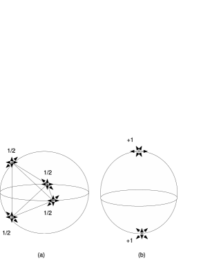
Figure 2: (a) The distribution of four surviving strategy with topological charge $+1/2$ on a 2-sphere. (b) Two surviving strategies with topological charge $W=+1$.

What we presented in the discussions above is the simplest case, there is only one output field with two input vectors. For the most general case, the output vector has $m$ components with $m$ input vectors. There exist a $m$ dimensional tangent vector field for every component of the output vector,

$$\phi^{i}=\partial^{p-1-a_{i1}}_{\gamma^{1}}\partial^{p-1-a_{i2}}_{\gamma^{2}}...\partial^{p-1-a_{im}}_{\gamma^{m}}{O}_{ut}(\vec{\gamma}),\\$$

where $\sum_{i}a_{i}=0.$ We can define a gauss map, i.e., an unit vector field $\vec{n}$ with $n^{a}={\phi^{a}}/{||\phi||},\;\;n^{a}n^{a}=1,$ where $||\phi||=\sqrt{\phi^{a}\phi^{a}}\;(a=1,2,...,m)$. Following the topological field theoryDuanSLAC , we can find a topological current,

$$\Omega=\sum_{i,j,...,k;a,b,...,c=1}^{m}\epsilon^{ij...k}\epsilon_{ab...c}\frac{{\partial}n^{a}}{\partial{\gamma_{i}}}\frac{{\partial}n^{b}}{\partial{\gamma_{j}}}...\frac{{\partial}n^{c}}{\partial{\gamma_{k}}},$$ (55)

where $(a,b,...,c=1,2,...,m)$, $(i,j,...,k=1,2,...,m)$, $\epsilon_{ab...c}$ is antisymmetric tensor. On even dimensional manifold, this topological current is exactly equivalent to the Riemanian curvature tensor which directly leads to the Gaussian curvature in two dimensions. Applying Laplacian Green function relation, it can be proved that $\Omega=\delta(\vec{\phi})D(\frac{\phi}{\gamma})$, where the Jacobian $D(\frac{\phi}{\gamma})$ is defined as

$$D(\frac{\phi}{\gamma})=\sum_{i,j,...,k;a,b,...,c=1}^{m}\epsilon^{ij...k}\epsilon_{ab...c}\frac{{\partial}\phi^{a}}{\partial{\gamma_{i}}}\frac{{\partial}\phi^{b}}{\partial{\gamma_{j}}}...\frac{{\partial}\phi^{c}}{\partial{\gamma_{k}}}.$$

In $m=2n$ dimensional manifold, it was proved that the topological charge of this current is the Chern number $Ch=\int{\Omega}d^{2}q=\sum_{k=1}^{l}{W_{k}}$, which is the sum of the winding number around the surviving strategies for multi-player game.

IV.2 The universal equation of coexistence curve in phase diagram

A phase transition is a war, is a game, is a revolution. No matter where it takes place, it becomes landmark in history of a system. The renormalization group transformation theory told us a phase transition point is the Nash equilibrium solution of a game. As shown in the bargain game, the profit of seller is the loss of the buyer and vice versa. When the seller takes proper strategies to maximize his profit, the buyer is trying to minimize it by taking strategies from a different space. So the seller is approaching to the maximal point of the payoff function, in the meantime the buyer is looking for its minimal point. A Nash equilibrium appears at their intersection. The Nash equilibrium point is a saddle point, the output field reaches its maximal point in $\gamma_{1}$ direction, but get a minimal value in $\gamma_{2}$ direction. The derivative of the output field corresponds to $\gamma_{1}$ and $\gamma_{2}$ must be of opposite sign. This leads to the coexistence equation for different phases.

In previous sections, when solving the equation of tangent vector field $\phi=0$ to find the surviving strategies, we applied a regular condition $D(\phi/\gamma)\neq 0$, which comes from the implicit function theoremgoursat . When the regular condition is violated, i.e., $D(\phi/q)=0$, a definite solution of equation $\phi=0$ is not available. Then the branch process of the solutions function occurs. A mathematical demonstration of the branch process could be found in Ref.DuanSLAC . This bifurcation may be understand from game theory. Under the regular condition $D(\phi/\gamma)\neq 0$, if the solutions of $\phi=0$ exist, that means the old phase still has strategies to survive, if there is no solutions, the old phase can not find any strategy to make a living, it has to die. When the regular condition fails, $D(\phi/\gamma)=0$, the old phase and new phase is at an equilibrium war, if the old phase win, it find ways to survive, if it loses, no surviving strategy exist, the old phase dies. Therefore, it is at the very battlefield of $D(\phi/\gamma)=0$, the two phases have equivalent power, nobody wins, nobody lose, but they are fighting against each other. Several roads branched out of this battlefield, to be or not to be, the old phase has to make a choice when passing this critical region.

In two dimensional input space, the coexistence curve equation $D(\phi/\gamma)=0$ is just the familiar Poisson bracket for the tangent vector field $\phi^{i}=\partial^{p-1-i_{1}}_{\gamma^{1}}\partial^{p-1-i_{2}}_{\gamma^{2}}...\partial^{p-1-i_{m}}_{\gamma^{m}}{O}_{ut}(\vec{\gamma})$,

$$\{\phi^{1},\phi^{2}\}=0.$$ (56)

It is an unification of the special coexistence equations of different order phase transition. As all know, in quantum mechanics, if two operator $\hat{A}$ and $\hat{B}$ commutate with each other, i.e., $[\hat{A},\hat{B}]=0$, they share the same eigenfunction. Eq. (56) means that the two classical field $\phi^{1}$ and $\phi^{2}$ are commutable at the phase transition point.

When the game has three players, the output field is a function of three parameters, each of them holds the life of an old phase. The three phases intersects with one another at the coexistence points which sit at the solutions of

$$\{\phi^{i},\phi^{j},\phi^{k}\}=0,$$ (57)

where $\{\phi^{i},\phi^{j},\phi^{k}\}$ is the generalized Poisson bracket. Its quantum correspondence id the Jacobi identity

$$[A,[B,C]]+[C,[A,B]]+[B,[C,A]]=0.$$ (58)

For a $n$-player game, we need to introduce a $n$-dimensional renormalization group transformation on the output manifold. The transformation operator expand the tangent vector space around the identity on the manifold. We denote a vector operator as $\vec{L}$, a group element is given by $U=e^{i\theta\vec{n}\cdot{\vec{L}}}$. The basic tangent vector field for phase transition is

$$\vec{\phi}=(\phi_{\gamma_{1}},\phi_{\gamma_{2}},...,\phi_{\gamma_{n}})=\frac{\delta^{p}[U(\theta)\delta{\langle 0|\hat{O}|0\rangle}]}{\delta\theta^{p}}|_{\theta=0}.$$

The most general definition of generalized Poisson bracketnambu for $n$ component vector field is

$$\{\phi^{1},\phi^{2},...,\phi^{n}\}=\frac{\partial(\phi^{1},\phi^{2},...,\phi^{n})}{\partial(\gamma_{1},\gamma_{2},...,\gamma_{n})}.$$ (60)

The coexistence surface equation for n-player game is the Jacobian field for n-component output field, it is equivalent to the n-dimensional generalized Poisson bracket,

$$\{\phi^{1},\phi^{2},...,\phi^{n}\}=\sum_{i,j,...,k}^{n}\epsilon^{ij...k}\frac{{\partial}\phi^{1}}{\partial{\gamma_{i}}}\frac{{\partial}\phi^{2}}{\partial{\gamma_{j}}}...\frac{{\partial}\phi^{c}}{\partial{\gamma_{n}}}=0.$$ (61)

This coexistence equation of $m$ vector field $\{\phi_{i},(i=1,2,...,m)\}$ may be decomposed as a group equation of two field equations $\{\{\phi^{i},\phi^{j}\}=0,i,j=1,2,...,m\}$ where $i$ and $j$ must runs over all component of the vector field.

In order to verify the universal coexistence curve equation, we take the two-phase coexistence equation $\{\phi^{1},\phi^{2}\}=0$ as an example, and apply it to thermodynamic physics. The output field is the difference of free energy $\hat{O}_{ut}(\gamma)=\delta{F}=F^{A}-F^{B}$, the input vector are temperature $\gamma_{1}=T$ and pressure $\gamma_{2}=P$. It will be shown, the universal coexist equation $\{\phi^{1},\phi^{2}\}=0$ unified all the coexistence equations in classical phase transitions.

We first verify the second order phase transition. The order parameter of the second order phase transition is $\phi^{1}=\partial_{T}\delta{F}$ and $\phi^{2}=\partial_{P}\delta{F}$, substituting them into the Jacobian vector

$$\{\phi^{1},\phi^{2}\}=D(\phi/q)=\frac{\partial\phi^{1}}{\partial{T}}\frac{\partial\phi^{2}}{\partial{P}}-\frac{\partial\phi^{1}}{\partial{P}}\frac{\partial\phi^{2}}{\partial{T}}=0,$$ (62)

and using the relations

$$\partial_{T}\partial_{T}{\delta}F = \frac{{C_{p}^{A}}-{C_{p}^{B}}}{T},\;\;\partial_{P}\partial_{P}{\delta}F=V(\kappa_{T}^{A}-\kappa_{T}^{B}),$$

$$\partial_{P}\partial_{T}{\delta}F = V(\alpha^{B}-\alpha^{A}),$$ (63)

we arrive

$$D(\phi/q)=\frac{V}{T}({C_{p}^{B}}-{C_{p}^{A}})(\kappa_{T}^{B}-\kappa_{T}^{A})-(V\alpha^{B}-V\alpha^{A})^{2}.$$ (64)

Recalling the Ehrenfest equations

$$\frac{dP}{dT}=\frac{\alpha^{B}-\alpha^{A}}{\kappa^{B}-\kappa^{A}},\;\;\;\;\frac{dP}{dT}=\frac{C_{p}^{B}-C_{p}^{A}}{TV(\alpha^{B}-\alpha^{A})},$$ (65)

it is easy to verify that the equation above is in consistent with the bifurcation condition Eq. (64). So the bifurcation equation $D(\phi/q)=0$ is an equivalent expression of the coexistence curve equation. The solution of this equation is a two dimensional coexistence surface, the Ehrenfest equations actually indicates the normal vector of phase A and B is of equivalent value with opposite direction, i.e., $|\vec{n}_{B}|=-|\vec{n}_{A}|$, that means they reach balance on this surface.

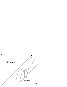
Figure 3: The saddle surface of the free energy around the critical point.

For the first order phase transition, we chose the vector order parameter as $\phi=\partial^{0}\delta{F}$, here ${}^{\prime}0^{\prime}$ means no derivative of the free energy. The generalized Jacobian vector of the first order phase transition with $\phi=\partial^{0}\delta{F}$ is given by

$$D(\frac{\phi}{q})=(\frac{\partial{F}^{B}}{\partial{T}}-\frac{\partial{F}^{A}}{\partial{T}})+(\frac{\partial{F}^{B}}{\partial{P}}-\frac{\partial{F}^{A}}{\partial{P}})=0,$$ (66)

in mind of the relation $\frac{\partial{F}}{\partial{T}}=-S$ and $\frac{\partial{F}}{\partial{P}}=V$, and considering $D(\frac{\phi}{q})=0$, we have

$$\frac{dP}{dT}=\frac{(S^{B}-S^{A})}{(V^{B}-V^{A})}.$$ (67)

This is the famous Clapeyron equation. The critical point is a saddle point. So it is the maximal point of free energy difference in $\gamma_{1}$ direction, and it is minimal point in $\gamma_{2}$ direction, their first order derivative must obey

$$\frac{d\delta{F}}{d\gamma_{1}}\frac{d\delta{F}}{d\gamma_{2}}<0.$$ (68)

The first order phase transition requires they must share the same absolute value at the critical point, then

$$\frac{d\delta{F}}{d\gamma_{1}}+\frac{d\delta{F}}{d\gamma_{2}}=0.$$ (69)

In fact, the free energy difference between the two sides of the coexistence acts as the phase potential, its first derivative is force, the force of the two phases must be of the same value but pointing in the opposite direction at the critical point.

The bifurcation equation $D(\phi/q)=0$ can be naturally generalized to a higher-order transition, it also leads to the coexistence curve of the higher order transition. We consider a system whose free energy is a function of temperature $T$ and magnetic field $B$, then the Clausius-Clapeyron equation becomes $dB/dT=-\Delta{S}/\Delta{M}$. If the entropy and the magnetization are continuous across the phase boundary, the transition is of higher order. For the $p$th order phase transition, the vector field is chosen as the $(p-1)$th derivative of $\delta{F}$, $\phi^{1}=\partial^{p-1}_{T}\delta{F},\;\phi^{2}=\partial^{p-1}_{B}\delta{F}$. Substituting $(\phi^{1},\phi^{2})$ into Eq. (62), we arrive

$$D(\phi/q)=\frac{\partial^{p}\delta{F}}{\partial{T}^{p}}\frac{\partial^{p}\delta{F}}{\partial{B}^{p}}-\frac{\partial\partial^{p-1}\delta{F}}{\partial{B}\partial{T}^{p-1}}\frac{\partial\partial^{p-1}\delta{F}}{\partial{T}\partial{B}^{p-1}}=0.$$ (70)

Considering the heat capacity $\frac{{\partial}^{2}F}{{\partial}T^{2}}=-\frac{C_{B}}{T}$ and the susceptibility $\frac{{\partial}^{2}F}{{\partial}B^{2}}=\chi$, the bifurcation condition $D(\phi/q)=0$ is rewritten as

$$\left[\frac{dB}{dT}\right]^{p}=(-1)^{p}\frac{\Delta\partial^{p-2}C/\partial{T}^{p-2}}{T_{c}\Delta\partial^{p-2}\chi/\partial{B}^{p-2}}.$$ (71)

This equation is in perfect agreement with the equations in Ref. kunmar .

In mind of our holographic definition of phase transition Eq. (39), we may also derive the holographic coexistence equation using the fundamental order parameter field,

$$\vec{\phi}=\frac{\delta^{p}[R(\theta)(F^{A}-F^{B})]}{\delta\theta^{p}}=\frac{\delta^{p}[R(\theta){\delta}F]}{\delta\theta^{p}},$$

$$R(\theta){\delta}F=\sum_{0}^{n}\frac{1}{n!}(\hat{L}\theta)^{n}{\delta}F,$$

$$\hat{L}={\gamma_{2}}\frac{\partial}{\partial{\gamma_{1}}}-{\gamma_{1}}\frac{\partial}{\partial{\gamma_{2}}}.$$ (72)

To study the $p$th order phase transition, one need to expand the group element $R(\theta)$ to the $p$ the order, and split it into the real part and imaginary part, i.e.,

$$\vec{\phi}={\frac{\delta^{p}[R(\theta){\delta}F]}{\delta\theta^{p}}}\bigr{|}_{\theta=0}=\phi^{1}+i\phi^{2}.$$

Then the coexistence curve equation is

$$\{\phi^{1},\phi^{2}\}=\frac{\partial\phi^{1}}{\partial{\gamma_{1}}}\frac{\partial\phi^{2}}{\partial{\gamma_{2}}}-\frac{\partial\phi^{1}}{\partial{\gamma_{2}}}\frac{\partial\phi^{2}}{\partial{\gamma_{1}}}=0.$$ (74)

Under this definition, it is easy to see that Kunmar’s result (71) is only special case of a series of coexistence equations for the $p$th order of phase transition, the complete coexistence curve equations are given by

$$\frac{\partial^{i}\delta{F}}{\partial{T}^{i}}\frac{\partial^{2p-i}\delta{F}}{\partial{B}^{2p-i}}-\frac{\partial^{j}\partial^{p-j}\delta{F}}{\partial{B^{j}}\partial{T}^{p-j}}\frac{\partial^{k}\partial^{p-k}\delta{F}}{\partial{T^{k}}\partial{B}^{p-k}}=0,$$

$$(i,j,k=1,2,...,p).$$ (75)

Now we see, the universal coexistence equation not only reproduced all the coexistence equations of classical phase transition in physics, but also gave more equations that have never been appeared before. This indicates that the game theory of renormalization group transformation has very broad applications.

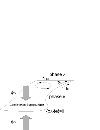
Figure 4: In analogy with Newtonian mechanics, the difference of output between two players is equivalent to gravitational potential $V$, the first order phase transition means the two phases have the same potential. For $p=2$, the order parameter field, $\phi^{A}=\partial^{p-1}_{\gamma_{A}}{O_{ut}},\;\phi^{B}=\partial^{p-1}_{\gamma_{B}}{O_{ut}}$, represents the force of phase A and B. When they reach balance, the two phase coexist on the hypersurface. This is the first order phase transition. For $p=3$, $\phi^{A}$ and $\phi^{B}$ represents the acceleration, although the force is not equal, but the acceleration are the same, this is the second order phase transition. On the two sides of the coexistence surface, the tangent vector are continuous, but the normal unit vector has a sudden jump.

For the magnetic field and temperature depended free energy $F(B,T)$, the scaling laws were derived in Ref. kunmar , the exponents is defined as

$$\frac{\partial^{p-2}C}{\partial{T}^{p-2}}=a^{-\mu},\;\;\;\frac{\partial^{p-2}\chi}{\partial{B}^{p-2}}=a^{-\kappa}.$$ (76)

The equivalent expression in terms of the vector field $\vec{\phi}$ is

$$\partial_{T}\phi^{1}=a^{-\mu},\;\;\;\partial_{P}\phi^{2}=a^{-\kappa}.$$ (77)

This scaling law is only a special case, there were many other scaling laws in various physical system, the same value of critical exponents falls into the same universality class. In the next section, we shall discuss the scaling laws based on the most general definition of phase transition.

IV.3 Universal scaling laws and coexistence equation around Nash equilibrium point

The phase transition of a physical system occurs at the critical point where the correlation length between particles becomes infinitestanley . It is assumed that the free energy is a generalized homogeneous function, i.e., $F(\lambda^{a}\gamma^{1},\lambda^{b}\gamma^{2})=\lambda{F}(\gamma^{1},\gamma^{2})$. The quantity defined by the free energy obey power laws around the critical point. From the two scaling exponent $a$ and $b$, one may derive those critical exponents which obey some equalities. The systems with the same scaling law fall into an universality class.

When it comes to the general phase transition defined as a war game in this paper, all the critical phenomenons in physical reappeared. During the war, the correlation between the all the members of the participants becomes infinity, people may not know each other, but every tiny work they do may cause great effect to the final results. If we focus on the individual person in battle field, one would see two opposite soldiers are fighting. Then we go to a larger scale, we see two companies are fighting. We can continue to magnify the scale, the participants who are fighting range from hundreds of people to millions of people, range from a small village to the whole world. No matter from which scale we see it, it is the same war. At the critical point, the participants of the war have equal strength, if any one of them make a tiny mistake(the mistake may come from an unimportant soldier), the whole army will lose the war, so the correlation length between soldiers goes to infinity. In this sense, the output field of the war should be a generalized homogeneous function at the critical point, it obeys the relation $\hat{O}_{ut}(\lambda^{i}\gamma_{i})=\lambda\hat{O}_{ut}(\gamma_{i})$.

According to the topological current of phase transition, we established the tangent vector field of $\hat{O}_{ut}$. The tangent vector field is the projection of physical field configuration on the strategy manifold. The physical field divergent at some singular points where the tangent vector field vanished. It was proved that the nontrivial Riemannian curvature just around these surviving strategy. The integral of the Riemannian curvature is a topological invariant, the critical exponent should bear a topological origin.

According to the universal definition of phase transition, the phase transition point is a Nash equilibrium solution. A special two dimensional output manifold is a saddle surface in the vicinity of the critical point. The output manifold is maximum for one parameter, but minimum for another parameter.

Suppose the topological dimension of the manifold around the critical point is integer, i.e., $D=1,2,...,n$, we may introduce a local coordinates to approximately express the output manifold in the vicinity of the critical point as

$$\hat{O}_{ut}=\frac{\kappa_{1}}{2}\gamma_{1}^{2}+\frac{\kappa_{2}}{2}\gamma_{2}^{2},$$ (78)

where $\gamma_{1}$ is the infinite small variable, based on which the local coordination is $r_{1}=(\delta{r}_{1}+\frac{1}{2}\Gamma_{ij}^{1}\gamma_{i}\gamma_{j})\sqrt{g_{ii}}+\cdots$. We may abandon the quadratic term of $\gamma_{i}$. Eq. (78) is the local approximation of the output manifold. $\kappa_{1}$ and $\kappa_{2}$ are principal curvature. When $\kappa_{1}>0$ and $\kappa_{2}>0$, it is a elliptic surface, when $\kappa_{1}>0$ and $\kappa_{2}=0$, it is parabolic, for $\kappa_{1}>0$ and $\kappa_{2}<0$, it is hyperbolic. Usually the local manifold on a two dimensional output manifold is hyperbolic at a phase transition point. In fact, if we carry out the derivative of Eq. (78) to the seconde order, it spontaneously leads to,

$$\partial^{2}_{\gamma_{1}}\hat{O}_{ut}={\kappa_{1}},\;\;\;\;\partial^{2}_{\gamma_{2}}\hat{O}_{ut}={\kappa_{2}},$$ (79)

they are actually intrinsic geometric constant of the neighbor manifold around the critical point.

Recall the game theory of renormalization group transformation in the first section, one would see that the game operator is a nonlinear operator, it defines an iterative map for the game process. The dimension of the infinite small neighboring manifold around the Nash equilibrium point can be exactly calculated from the game operator. For most nonlinear game operators, the dimension of the manifold around the Nash equilibrium is fractal instead of integer. There are only a few very simple cases that one can find an integer dimension. But the game operator in that cases is too trivial to give us any interesting phenomena. According to the experiments and numerical calculation of physics, we can make a general hypothesis that the neighboring output manifold around the critical point of phase transition, namely around the Nash equilibrium point of a non-cooperative game, has fractal dimension.

In the vicinity of the phase transition point,an approximation of the scale invariant output manifold is a complex function in fractal space,

$$\hat{O}_{ut}(\gamma)=\kappa_{i}\gamma_{i}^{d_{i}}+\kappa_{m}[f(\gamma_{j}^{d_{j}}+\gamma_{k}^{d_{k}}...)]^{d_{m}}+\ldots,$$ (80)

where $d_{1},d_{2},...,d_{n}$ are fractal dimensions wit respect to different input parameters. Recall that most of the physical observables in statistical mechanics are defined by the second order derivative of free energy, we can define the observables of a complex system by the second order derivative of the output field. The free energy is only a special component of the output manifold in physics. When we study the most general complex system, as long as people can measure it, we can take any order of derivative of the output field as observables. These observables are just the components of the tangent vector field of the output field. A simple example of the tangent vector field is

$$\phi_{ij}=\frac{\partial^{2}\hat{O}_{ut}(\gamma)}{\partial{\gamma_{i}}\partial{\gamma_{j}}}={d_{i}}\gamma_{i}^{d_{i}-1}+d_{j}\gamma_{j}^{d_{j}-1}+\cdots.$$ (81)

According to the topological phase transition theory, the tangent vector field satisfy the phase coexistence equation $\{\phi^{1},\phi^{2},...,\phi^{n}\}=0$ at the critical point, we can derive a constrain on these vector field. We substitute the explicit expansion of the observable quantities into the coexistence equation, it would lead us to a constrain on the fractal exponent index. These constrain relations are just the scaling laws. Therefore scaling laws come from the coexistence equation of the crossing defined physical quantities.

The scaling relations found in various physical system are probably the simplest relations on the fractal space extended by two parameters. One can reach all kinds of different scaling relationsstanley in statistical mechanics by taking the output field as free energy $\hat{O}_{ut}(\gamma_{i})=F(\gamma_{i})$, and taking the input $\gamma_{i}$ as physical parameters, such as temperature $T$, pressure $P$, magnetic field $B$, and so on. In the vicinity of a second order phase transition, the divergent physical quantity are defined by the second order derivative of the free energy. Such as the susceptibility $\chi=-\partial^{2}F/\partial{H}^{2}$, $H$ is magnetic field. Each divergent quantity is characterized by a critical exponent, this critical exponent comes from fractal space. The two component coexistence $\{\phi^{1},\phi^{2}\}=0$ produced the scaling relations, such as the Fisher relation $\nu{d}=2-\alpha$, Widom relation $\hat{{\gamma}}=\beta(\delta-1)$, Rushbrooke relation $\alpha+2\beta+\hat{\gamma}=2$, and so on. We take the Rushbrooke relation as example to verify the coexistence equation. The Gibbs free energy is $G=U-TS$, its differentiation is $dG=-SdT+VdP-MdH$. Experimental and numerical calculation found that three thermodynamic quantity obey the following scaling laws in the vicinity of critical point,

$$M = -(\frac{\partial{G}}{\partial{H}})\sim{|T|}^{\beta},$$

$$C_{P} = -T(\frac{\partial^{2}G}{\partial{T}^{2}})_{P,H}\sim{|T|}^{-\alpha},$$

$$\chi = -(\frac{\partial{G}}{\partial{H}})\sim{|T|}^{-\gamma}.$$ (82)

The fundamental vector field can be taken as

$$\phi^{1}=(\frac{\partial{G}}{\partial{H}}),\;\;\;\;\;\phi^{2}=(\frac{\partial{G}}{\partial{T}}).$$ (83)

Substituting the two vector field into the coexistence equation $\{\phi^{1},\phi^{2}\}=0,$ one may derive

$$\frac{\partial^{2}{G}}{\partial{T}^{2}}\frac{\partial^{2}{G}}{\partial{H}^{2}}-\frac{\partial^{2}{G}}{\partial{T}\partial{H}}\frac{\partial^{2}{G}}{\partial{H}\partial{T}}=0.$$ (84)

Now we substitute the thermodynamic quantities (IV.3) into the coexistence equation, it yields

$${|T|}^{-\alpha-\gamma}=\beta^{2}{|T|}^{2\beta-2}.$$ (85)

When $T\rightarrow 0$, we may ignore the coefficient $\beta^{2}$ at the right hand side of Eq. (85), then we obtained the Rushbrooke relation $\alpha+2\beta+\hat{\gamma}=2$. Other scaling relation can be verified following similar procedure. These relations were firstly found by computational simulation and experiments. Therefore the scaling law of universal phase transition in a general complex system has solid numerical and experimental foundation. Here it must be pointed out that the commutable relation $\partial_{T}\partial_{H}=\partial_{H}\partial_{T}$ have been used in the calculation. This suggests that the partial differential corresponding to different variables are commutable in the vicinity of critical point. This is in consistent with our picture of war game at the phase transition point. Further more, one may choose different tangent vector field for the coexistence equation, then one may obtain all different scaling relations in the vicinity of critical point.

IV.4 The symmetry of Landau phase transition theory and symmetry of game theory

The Landau theory of continuous phase transition theory provides a basic description to the phase transition characterized by spontaneous symmetry breaking. Take its application to the structure phase transitions as one example, it derives several important features, namely, the change in the crystal’s space group, the dimension and symmetry properties of the transition’s order parameter, and the form of the free energy expansion. It has the same range of validity as the mean-field approximation in microscopic theories. A central assumption of the Landau theory is that the free energy can be expanded as a Taylor series with respect to the order parameter $\eta$:

$$F(P,T,\eta)=F_{0}+A(P,T)\eta^{2}+B(P,T)\eta^{3}+C(P,T)\eta^{4}+...$$ (86)

in which the phases are marked by the order parameter $\eta$. The symmetry in Laudau theory talks about the invariance of this free energy when we do some transformation on the order parameter field $\eta^{\prime}\rightarrow{U}\eta$. This symmetry is the same conception as that in quantum field theory, such as the $\psi^{4}$ model, $\mathcal{L}=\frac{1}{2}(\partial_{\mu}\psi)^{2}-\frac{1}{2}m^{2}\psi^{2}-\frac{\lambda}{4}\psi^{4}$. If the equations of motion derived from this Lagrange is invariant under some transformation $\psi\rightarrow\psi^{\prime}$, we call such a transformation a symmetry transformation.

But in this paper, the symmetry we are talking about in the game theory of phase transition is a different conception.

The object of our research is a very general system $\vec{O}_{ut}=F_{out}(\vec{x},\vec{\gamma})$, $\vec{\gamma}$ is the input vector. In game theory, the input vector represent the input strategies of different players. In physics, the input vector are physical operational quantity. $\vec{O}_{ut}$ is output vector, it encompasses all the information the observer can received by sending different inputs. In physics, the outputs are physical observables. The state $\vec{x}$ represent the inner states of system, it plays a similar role as the order parameter field $\eta$ in the free energy expansion equation (86). In our game theory of topological phase transition theory, all the state vector have been integrated out, the fundamental starting point is the output field $\vec{O}_{ut}=F_{out}(\vec{\gamma})$, the symmetry we mentioned in this theory is about the transformation invariant property of $\vec{O}_{ut}$ under the transformation $\vec{\gamma}^{\ast}\rightarrow{U}\vec{\gamma}$. For example, in the free energy equation (86), $F(P,T)$ is output, $P$ and $T$ are the two players, we study the symmetry of $F(P,T)$ when $T\rightarrow{T}^{\prime}$ and $P\rightarrow{P}^{\prime}$. The order parameter $\eta$ is not an operation quantity, it describes the inner state of the system.

The Landau theory of phase transition can be summarized as a differential game(see Appendix D,E). The order parameter is the state vector of the game. In the frame work of our topological current theory of phase transition, the tangent vector field $\phi^{i}$ consists of the complete set of phase dynamics system. The vector field

$$\phi^{i}=\partial^{q-1}_{P}\partial^{p-1}_{T}(\frac{{\delta}F(P,T,\eta)}{\delta\eta})$$ (87)

describes how the two player $T$ and $P$ behave across the state vector space $\eta$. The free energy is the output function. $F(P,T,\eta)$ should be written as an expansion in the even powers in the spirit of Gintzburg-Landau formalism, for $F(P,T,\eta)$ must be gauge invariant with respect to the order parameter $\eta$. Then the series of free energy in even powers truncated at the fourth order is

$$F(P,T,\eta)=F_{0}+A(P,T)\eta^{2}+C(P,T)\eta^{4},$$ (88)

A special phase vector field may be chosen as

$$\phi^{1}=2\partial^{1}_{T}[A(P,T)+2C(P,T)\eta^{2}]\eta,$$

$$\phi^{2}=2\partial^{1}_{P}[A(P,T)+2C(P,T)\eta^{2}]\eta.$$ (89)

If $\phi^{1}$ and $\phi^{1}$ do not commute with each other, both the two players have surviving strategy which are the solutions of $\phi^{1}=0,\;\phi^{2}=0$, these solution sit at some isolated points

$$T_{k}=T_{k}(\eta),\;\;P_{k}=P_{k}(\eta),\;\;k=1,2,...,l,$$ (90)

Each of these isolated solutions has a winding number $W_{k}$. These surviving strategy pair ($T$,$P$) are changing according to the state vector $\eta$. The surviving strategy of new phase and old phase carry opposite winding number, they are annihilating and generating at the phase coexistence region. The sum of these winding number is a topological quantity which is determined by the topology of the state vector manifold. .

Usually $A(T,P)$ has the form of $a(P)(T-T_{c})$ near the critical temperature $T_{c}$, and C(P,T) is supposed to be weakly dependent on the temperature, i.e., $\partial_{T}C\ll 1$. Considering Eq. (IV.4), the surviving strategy for the old phase and new phase can be derived from

$$\eta[a(P)+2\partial_{T}C(P,T)\eta^{2}]=0,$$

$$\eta[\partial_{P}a(P)(T-T_{c})+2\partial_{P}C(P,T)\eta^{2}]=0.$$ (91)

One sees that $\eta=0$ corresponds to a stable phase solution of the equation above. For the case $\eta\neq 0$, there are two solutions:

$$\eta=\pm\left[\frac{-a(P)}{2\partial_{T}C}\right]^{1/2},\;\eta=\pm\left[\frac{\partial_{P}a(P)(T_{c}-T)}{2\partial_{P}C}\right]^{1/2},$$ (92)

if we chose $C=exp({T+P})$ and $a=exp(P)$, it turns into a familiar form

$$\eta_{1}=\pm\left[\frac{-a(P)}{2C}\right]^{1/2},\;\eta_{2}=\pm\left[\frac{a(P)(T_{c}-T)}{2C}\right]^{1/2}.$$ (93)

The coexistence curve equation $\{\phi^{1},\phi^{2}\}=0$ is an universal equation, it holds for this two player game. Consider the two special vector field Eq. (IV.4), we arrived a sophisticate coexistence equation,

$$4\eta^{2}\partial^{2}_{T}C[\partial^{2}_{P}A(T,P)+2\partial^{2}_{P}C\eta^{2}]=[\partial_{P}a(P)+2\partial_{P}\partial_{T}C\eta^{2}]^{2}.$$

If we have obtained the explicit relation of $A(T,P)$ and $C(T,P)$, then we can depict the phase diagram in $T-P$ plane for different state vector $\eta$.

IV.5 Symmetry and evolution of phases in game theory

In game theory, the output vector are payoff functions, the inputs are strategies. A symmetry transformation in strategy space does not always lead to different output, the Nash equilibrium solution is invariant fixed point under continuous transformation. As shown in Ising model, the renormalization group transformation keep mapping a pair of strategy to another pair, no matter where it starts, it always flows to the fixed point.

The phase of a system evolutes in the direction of renormalization group transformation flow. The direction of renormalization group transformation flow is determined by the Second Law of Thermodynamics, which states all physical systems in thermal equilibrium can be characterized by a quantity called entropy, this entropy cannot decrease in any process in which the system remains adiabatically isolated. We can ignore the thermodynamics, and grab the central point that an isolated system only evolutes in the direction of increasing entropy. This statement of the Second Law of Thermodynamics may also hold in game theory, but notice that the entropy here in our theory is not the conventional conception defined in statistical physics, since we are not manipulating the physical particles, it is the entropy of players $\vec{\gamma}$ instead. In physics, the players are those physical observables. An isolated system evolves spontaneously toward a maximal symmetry.

The entropy of the multi-player game measures indistinguishability of players. Let’s look at an ancient battlefield with two armies ready to fight, before the beginning of the combat, the two troops are organized in ordered states separated by vacant glacis, every part of them has special functioning. A bystander can tell which is which. Once the combat begins, they rush at each other and fused into one. In this case, the bystander is unable to distinguish them, it is completely in chaos. When the war finished, the loser surrendered, winner gathered, the two troops translated into another ordered states. The surviving troops are distinguishable again, but those dead can never be back to ordered states again.

High symmetry leads to high entropy. If we do some transformation to a system in chaos, it won’t make any difference. As in the war, the two armies become a mixture, it is an unstable equilibrium state with the highest symmetry. The higher symmetry a system owns, the more unstable it would be. The state before and after the war are both of less symmetry states. Like the beginning of universe, all different conflicting interactions confined in a singular point, reach an unstable equilibrium state. It has the highest space time symmetry. A minor imbalance results in the Big Bang. The explosion breaks the singularity apart into all different symmetry zone. Each symmetry group brings about a stable phase.

The stable phases at different stage of history may be found following the group chain of the original symmetry group. A high symmetry group usually has a series of subgroup. A physical system liken to stay in the most fundamental symmetry state. People love peace, but hate war. They like to live at the most stable point of the system. A war cost too much energy. The subgroup chain of a given group is always finite,

$$U\supset{U_{1}}\supset{U_{2}}\supset{U_{3}}...\supset{U_{p}}.$$ (94)

For example, $SO(4,2)$ constitutes a dynamical group for the Hydrogen atomnambu . It has many four subgroupsbrian ,

$$SO(4,2)\supset{SO(4,1)}\supset{SO(4)}\supset{SO(3)}\supset{SO(2)}.$$ (95)

This group chain may be followed by point group. For instance, the $U(1)$ symmetry group may be decreased to $T_{n}$ which means a physical system is invariant when it rotates $\frac{2\pi}{n}$ around one axel. So we can roughly find the stable phase according to the group chain. Generally speaking, Lie group is highes rank of group. The discrete group are imbedded in Lie groups. The most stable phase focus on the lowest symmetry.

A game system evolutes following the first principal, the players take different strategies to ground state. The $N$ players represents $N$ interaction, or $N$ input vectors. In the beginning, each of them occupies a small domain in phase diagram and is the ruler in his own domain. There is temporary balance between the different players. The war is going on all the time between neighboring domains. Whenever a player loses, he dies out, his enemies absorbed his domain. When a player fails, an old phase died, and a new phase is born, this indicates a phase transition. The balance on the boarder between different domains represent the phase coexistence region, on which Nash equilibrium is reached. But this state is an unstable equilibrium state, there is constantly minor conflicting to destroy this balance. Then the war goes on, the winners gain advantage, and becomes stronger and stronger, the war will not stop until he unified the domains as one.

The phase diagram of a physical system is depicted in the frame of some static physical parameter. We can view the evolution of phase as an continuous tuning of the physical parameter. For example, if we continuously raise temperature, we will see single curve in the phase diagram bifurcates at certain temperature, this is the evolution of physical phase, although it is not the usual evolution in the common sense of time.

This phase evolution with respect to temperature can be viewed as a generalized dynamic process in parameter space. As shown in section (III.2), a multi-player game can be equivalently expressed as a group of differential equations. The evolution of output vector $\vec{O}_{ut}$ is governed by the differential equations,

$$\partial_{s}\vec{O}_{ut}=\hat{L}(\gamma,\partial_{\gamma})\vec{O}_{ut},\;\;\;\;\;i=1,2,...,n.$$ (96)

If we take the tuning parameter $s$ as temperature $T$, then we understand the evolution of phase with respect to temperature. In physical system, we can obtain the function of linear response by perturbation theory. The response function $\vec{O}_{ut}$ may have sophisticate relation with input parameters, $\vec{O}_{ut}(\gamma)$. Some input parameters are function of temperature $\gamma_{i}=\gamma_{i}(\gamma_{j})$. For example, during the isothermal process, the product of pressure and volume is a constant $PV=constant$, so $P$ and $V$ are related by this equation. We take the $\gamma_{i}(\gamma_{j})$ as fundamental variables, $\gamma_{j}$ is the tuning parameter. Then the generalized momentum is defined as

$$P_{\gamma_{i}}=\frac{\partial{\phi(\gamma,\partial_{\gamma_{j}}\gamma,\gamma_{j})}}{\partial{(\partial_{\gamma_{j}}\gamma^{i})}},$$ (97)

where $\phi(\gamma,\partial_{\gamma_{j}}\gamma,\gamma_{j})$ is a reference function like Lagrangian function. We can further find a vector field $\phi_{H}(\gamma,\partial_{\gamma_{j}}\gamma,\gamma_{j})$ which is similar to the Hamiltonian function in Lagrangian mechanics. For a given field $\phi_{H}$, the game operator $\hat{L}(\gamma,\partial_{\gamma})$ bear an expression in terms of Poisson bracket,

$$\hat{L}(\gamma,\partial_{\gamma})=\frac{\partial\phi_{H}}{\partial{P_{\gamma_{i}}}}\frac{\partial}{\partial{\gamma}}-\frac{\partial\phi_{H}}{\partial{\gamma}}\frac{\partial}{\partial{P_{\gamma_{i}}}}.$$ (98)

This formula of game operator leads to another equivalent representation of the differential equation ,

$$\partial_{\gamma_{j}}{O}_{ut}=\{\phi_{H},{O}_{ut}\}.$$ (99)

This equation actually describes the game process between $\phi_{H}$ and ${O}_{ut}$, each of them navigates one stable phase. If they are in the same complete set, $\{\phi_{H},{O}_{ut}\}=0$, then the two phases coexist. In fact, the Hamiltonian function does not play any special role in our topological current theory of phase transition, it is just one of the tangent vector field in Lie algebra space.

IV.6 Phase coexistence boundary and unstable vacuum state

As we defined in the beginning, phase transition is a transition from one stable state to another stable state, there is a critical point at which the old stable state collapsed and the new state arise from the shambles and grow to a stable state. A oversimplified model is take two states as a vector of two component $(x,y)$, the evolution operator is a diagonal 2 by 2 matrix $\hat{L}=\texttt{diag}(-1,1)$ at the coexistence region. The evolution of the two phase follows the equation $\partial_{\gamma}\vec{r}=\hat{L}\vec{r}$, which we established in last section. Then in the vicinity of the coexistence region, we would see the old phase decays following $x\propto{e^{-a\gamma}}$, in the meantime the new phase blows up $y\propto{e^{+a\gamma}}$, where $a>0$.

The mechanical simulation of the phase coexisting state is a ball on the maximal tip of the parabola $f(z)=-z^{2}$. At Nash equilibrium point, a player take the best strategy to minimize his own damage, and obtain his maximal profit in the meantime. In fact, it is the profit difference between them that they fight for. When the two conflicting force reach a balance, the game arrived at a Nash equilibrium.

The Nash equilibrium state is an unstable maximal point in the mechanical potential of the output field. Let $\hat{O}_{ut}^{i}(\vec{\gamma})$ be the output function of the player $\gamma^{i}$, the effective potential for two players in a game is $\Delta{O}_{ij}=\hat{O}_{ut}^{i}(\vec{\gamma})-\hat{O}_{ut}^{j}(\vec{\gamma})$. Nash equilibrium sits at the minimal point of $|\delta{O}_{ij}|$. Notice that the player $\gamma^{i}$’s profit is the damage of player $\gamma^{j}$, so $\Delta{O}_{ij}=-\Delta{O}_{ij}$. We may establish a general equation of motion for player $\gamma^{i}$’s profit function,

$$\partial^{2}_{{\gamma}^{i}}\hat{O}_{ut}^{i}=\partial_{{\gamma}^{i}}V(\hat{O}_{ut}^{i}),$$ (100)

$V(\hat{O}_{ut}^{i})$ is a general potential which is self-consistently decided by other players, usually the player $\gamma^{i}$ sits at some of its minimal points, while the other players occupied its maximal point. The typical profit function $\hat{O}_{ut}^{i}$ of player $\gamma^{i}$ is a kink solution,

$$\hat{O}_{ut}^{i}=\pm\tanh(\gamma^{i}-\gamma^{\ast})=\frac{e^{\gamma^{i}-\gamma^{\ast}}-e^{\gamma^{\ast}-\gamma^{i}}}{e^{\gamma^{i}-\gamma^{\ast}}+e^{\gamma^{\ast}-\gamma^{i}}}.$$ (101)

where $\gamma^{\ast}$ is the optimal strategy. Eq. (101) is the familiar kink solution of quantum tunnelling problemskleinert . Any minor deviation from the Nash equilibrium solution would results in drastic increase or decrease of the profit function. Therefore the Nash equilibrium solutions of a game play the same role as the vacuum solution to quantum tunnelling. A collection degenerate vacua means there are a series of Nash equilibrium solutions with the same optimal value.

The game of phase transition has two different equilibrium states. One is all different interactions reach an agreement to maintain peace, this is the optimal strategy of cooperative game. It is the trivial vacuum. The other is that no peace agreement is derived, a war breaks out. At the critical point, different phases coexisted but against each other. This is the Nash equilibrium state. It is an unstable vacuum state.

The coexistence equation of $n$-different phases we obtained in previous sections,

$$\{\phi^{1},\phi^{2},...,\phi^{n}\}=0,$$ (102)

describes a Nash equilibrium state, or in other words, the coexisting unstable vacuum state, here $\vec{\phi}=(\phi^{1},\phi^{2},...,\phi^{n})=\frac{\delta^{p}[U(\theta){O}_{ut}]}{\delta\theta^{p}}{|}_{\theta=0}$. For this equation is antisymmetric, exchanging any two of the players would add a $(-1)$ to the output. As shown in the topological current of phase transition, the sum of the winding numbers around the surviving strategies is a topological number—-Chern number. The sign of each winding number is determined by the sign of $\{\phi^{1},\phi^{2},...,\phi^{n}\}$. Every $\phi^{i}$ field is a player, if exchange any two of them, the winner becomes loser, the loser turns into winner. Therefore if $\phi^{i}$ has a positive winding number, his opponent must has a negative one. The strategy for $\phi^{i}$ to survive is the anti-strategy of his opponents. During phase transition, the old phase is the opponent of the new phase. The winding number of the new phase’s strategy $\gamma^{j}$ is $W^{j}_{New}>0$, the winding number around the surviving strategy $\gamma^{i}$ of the old phase is $W^{i}_{Old}<0$. The topological constrain suggests

$$N_{ChernNumber}=\sum_{i}W^{i}_{Old}+\sum_{j}W^{j}_{New}.$$ (103)

We may view each strategy of the new phase as one particle with topological charge $W_{New}$, and its corresponding anti-particle is the anti-strategy of the old phase which carries a negative winding number. The soldiers of the new phase are the strategies, they carry positive winding number, rush at the coexist curve to fight against the anti-strategy of the old phase. The particles and antiparticles annihilate at the phase boundary, so the coexisting phase boundary behaves as vacuum. This war is going on under the constrain of Eq. (103).

The generator of translation group along $\gamma^{\mu}$ is $i\partial_{\gamma^{\mu}}$. The evolution of the output on the strategy space follows the classical Hamiltonian-Jacobi equation,

$$i{\partial_{\gamma^{\mu}}{\langle\hat{O}_{ut}(\theta)\rangle}}=\{\langle\hat{O}_{ut}(\theta)\rangle,\;L\},$$ (104)

The second quantization of this equation is just the Heisenberg equation $i\partial_{t}\hat{O}_{ut}=[\hat{O}_{ut},H]$, which has a more general covariant form

$$i\partial_{\gamma^{\mu}}{\hat{O}_{ut}}=[\hat{O}_{ut},\hat{P}_{\mu}],$$ (105)

here ${\gamma}^{\mu}=(t,\vec{\gamma})$, $P_{\mu}=(H,\vec{P})$. In four dimensional Minkoveski space time, the Hamiltonian is the generator of translation group with respect to time $t$. While the momentum operator $\hat{P}_{\mu}$ is the generator of space translation group. Integrating the covariant Heisenberg equation (105), we arrive

$$\hat{O}(\gamma)=e^{i\hat{P}\gamma_{\mu}}\hat{O}(0)e^{-i\hat{P}\gamma_{\mu}}.$$ (106)

If the output is expressed by quantum operators, its evolution in strategy space is governed by renormalization group transformation

$$U(\theta)\langle\hat{O}\rangle{U}^{-1}(\theta)=e^{i\theta\vec{n}\cdot{\vec{L}}}\langle\hat{O}{\rangle}e^{-i\theta\vec{n}\cdot{\vec{L}}}=\langle\hat{O}\rangle+i\theta\;[\vec{n}\cdot{\vec{L}},\;\langle\hat{O}\rangle]+\frac{(i\theta)^{2}}{2!}[\vec{n}\cdot{\vec{L}},\;[\vec{n}\cdot{\vec{L}},\;\langle\hat{O}\rangle]]+\cdots.$$ (107)

For the most simple Lie group $SO(2)$ whose Lie algebra has only one generator $\hat{L}_{z}$, this transformation equation takes a very simple form,

$$U\delta\langle\hat{O}\rangle{U}^{-1}$$

$$=\delta\langle\hat{O}\rangle+i\theta\;[\hat{L}_{z},\;\delta\langle\hat{O}\rangle]+\frac{(i\theta)^{2}}{2!}[\hat{L}_{z},\;[\hat{L}_{z},\;\delta\langle\hat{O}\rangle]]+\cdots.$$

In quantum mechanics, if a group transformations $U$ commutes with Hamiltonian $\hat{H}$, $[U,H]=\hat{H}U-U\hat{H}=0$, i.e., $H=H^{\prime}=U\hat{H}U^{{\dagger}}$, then $\hat{H}$ is invariant under transformation of group $U$, they share the same eigenfunction. In a general game theory, the Hamiltonian has nothing special. The generators of Lie algebra plays the role of Hamiltonian operator. The quantization of the coexistence equation reads

$$[\hat{\phi}^{1},\hat{\phi}^{2},...,\hat{\phi}^{n}]=0.$$ (108)

Each operator $\hat{\phi}^{i}$ represents a quantum operator, if they commute with each other, they share the same eigenspace. Eq. (108) is the quantum coexistence equation.

If the $\hat{\phi}^{i}$ are vectors expanded in the tangent space of Lie group around the identity, they are vectors of Lie algebra. For Mathematician, this coexistence equation corresponds to an invariant Cartan space of Lie algebra. The coexistence phase space is the eigenspace of Cartan subalgebra. The Cartan subalgebra is the maximal Abelian subalgebra. An arbitrary Lie algebra vector commuting with this subalgebra is still a Lie vector in the same space. The elements $C_{j}$ in this commutative subalgebra must satisfies

$$[C_{i},C_{j}]=0,\;\;\;\;(i,j=0,1,2,...,l).$$ (109)

$l$ is the dimension of the Cartan subalgebra space. It is also the number of coexistence phases. For the coexisting point of three phases, we define the three operator commutator as

$$\;\;\;[C_{i},C_{j},C_{k}]$$

$$=[C_{i},C_{j}]C_{k}+[C_{j},C_{k}]C_{i}+[C_{k},C_{i}]C_{j}$$

$$=0,\;\;\;\;(i,j,k=0,1,2,...,l).$$ (110)

It has a straight forward generalization for the points at which $n$ phases intersects,

$$[C_{i},C_{j},C_{k},...,C_{f}]=0,\;(i,j,k,...,f=0,1,2,...).$$ (111)

So we have a well defined quantum operator

$$\hat{D}^{n}=[\hat{\phi}^{1},\hat{\phi}^{2},...,\hat{\phi}^{n}],$$ (112)

This operator is defined from by vectors of Lie algebra, we call it phase coexistence operator. According to the group representation theorychenjq , we can always find the representation of coexistence operator,

$$\hat{D}^{n}|\psi_{n}\rangle=D|\psi_{n}\rangle.$$ (113)

If $n=2$, $\hat{D}^{n}$ is just the commutator of two operators which represent two stable phases. The phase boundary between phase $A$ and phase $B$ is given by the zero modes of the commutator of the two phase operators. When $\hat{\phi}_{A}$ and $\hat{\phi}_{B}$ are not commutable, the eigenfunctions of the phase coexist operator may be divided into positive modes and negative modes,

$$\hat{D}^{n}|\psi_{n}\rangle=sign{W}|\psi_{n}\rangle.$$ (114)

in which $W$ is the winding number around the surviving strategy. $sign(W)=+1>0$ corresponds to stable phase A and $sign(W_{pt})=-1<0$ corresponds phase B, while $(W_{pt})=0$ indicates the phase boundary. One of the most familiar example is to take the phase operator as the three component of angular momentum operator, $\hat{\phi}_{A}=L_{x}$ and $\hat{\phi}_{B}=L_{y}$, then $\hat{D}^{2}=L_{z}$. $L_{z}|\psi_{m}\rangle=m|\psi_{m}\rangle$, $m=\{0,\pm\}$. $m=0$ is the coexistence eigenvalue, $m=\pm 1$ represents the two stable phases.

In topological quantum field theory, the topological information of the zero mode is described by the Atiyah-Singer index theory. The strategy space of the game of phase transition can be split into positive eigenspace and negative eigenspace. The surviving strategies of the new phase carry positive winding number, we call them positive modes $\phi^{+}$. The strategies of the old phase is the enemy of new phase, they carry negative winding number, so we call them negative modes $\phi^{-}$. As shown by Eq. (51), our topological current theory of phase transition proved that the Euler characteristic number on two dimensional strategy space is,

$$Ch = \int\delta^{2}(\vec{\phi}_{+})\{\phi_{+}^{1},\phi_{+}^{2}\}-\int\delta^{2}(\vec{\phi}_{-})\{\phi_{-}^{1},\phi_{-}^{2}\},$$ (115)

$$= \sum_{i}W^{i}_{+}-\sum_{j}W^{j}_{-}.$$

For the 2n-player game, the topological Chern number on this $2n$ dimensional strategy manifold is determined by Atiyah-Singer theorem,

$$Ch_{B_{i}}=Index\hat{D}^{n}=dim\hat{D}_{+}^{n}-dim\hat{D}^{n}_{-},$$ (116)

where $\hat{D}^{n}$ is th quantized phase coexistence operator. The positive modes behaves as particles, and the negative modes are antiparticle, they coexist in vacuum. They are born by pairs from vacuum, and annihilate by pairs to vacuum.

In the language of Atiyah-Singer index theorem(see appendix section I), the topological index is the difference between the number of positive eigen-modes and negative eigen-modes. The positive modes is the surviving strategy for the new phase, the negative modes is the surviving strategy for the old phase. Thus the topological index counts how many extra strategies the new phase have after his soldiers rushed at front and annihilated at the coexistence phase boundary. We first assume every surviving strategy has a topological $|W|=1$ for convenience, the Euler number $Ch=+2$ on a sphere, this topological constrain says that when all the soldier of the old phase died, there are at least two positive soldiers of the new phase left. The victory of the new phase has been determined by topology of the strategy manifold. If it is on a torus, the Euler number is zero, $Ch=0$. The new phase is not that lucky now, his total number of soldiers is identical with that of the old phase. When the war break out, the strategy-anti-strategy pair annihilate on the phase coexistence boundary, the final result is a draw. When the base manifold of strategy space is a torus with $n$-holes , the Euler number is $Ch=2(1-n),n>1$, the final victory goes to the old phase, he has at least $2(1-n)$ surviving soldiers when the new phase is extinguished.

V Phase transition and entanglement in game theory

V.1 Phase transition and entanglement

The participants of a war entangled with each other before the war breaks out, otherwise there will not be a war at all. In fact, a game is played by many interacting players. During the game, a player choose strategy according to other players’ strategy, so he could never be a free particle unless he is not in the game.

The entanglement we are talking about here is a much more general conception, it includes the relation, interaction or connection between the elements of a system. The quantum entanglement in physics is one special case.

When the players are at peace, the entanglement between them is kept at a stable level. As the imbalance between different players increase, the war is coming, their entanglement grows stronger and stronger. The whole system becomes more and more unstable. When the critical point arrived, a negligible event trigged the war, which spread the whole system through the strong entanglement. During the war, all the players summon up their internal strength to collect information from all the other players, and make the best strategy to win the war, the entanglement reach a climax. The external response during the war also reached the strongest level. When the war is over, everything is in order, their entanglement gradually decay to another stable level.

Therefore, phase transition occurs when the entanglement between different phases reaches a maximal point. Every local maximal point of the entanglement indicates a transition, or a war. In order to give an exact prediction on where or when the war arise, we need to find some detectable quantity to measure the entanglement. So that we can quantitatively determine the position of the phase transition point.

The most familiar quantity for physicist is the von Neumann entropy. Quantum statistics suggests that the von Neumann entropy of a pure ensemble is zero. Entropy is a quantity to measure how disorder a system is. More disorder means higher entropy. The von Neumann entropy measure the disorder of the mixed states. The von Neumann entropy is a relatively small quantity if the system is in a stable phase. When the phase transition occurs, it would reach a climax point.

In fact, any sensitive output function corresponding to a group of inputs can be used as measure of entanglement. If the inputs have strong relation between them, one minor change would definitely change the others, and this would leads to the response of many outputs. One can see this from a war, it is at the war that the ignorable individuals began unite to work as a team, they are strongly correlated and entangled.

In our topological current of phase transition, a quantity to measure entanglement may be defined as

$$E_{ent}=\frac{1}{2\sqrt{\pi{h}}}\exp{[-{D(\phi/\gamma)}/(4h)]}$$ (117)

where $D(\phi/\gamma)=\{\phi^{1},\phi^{2},...,\phi^{n}\}$ is the coexistence equation, and $h$ is step size of renormalization group transformation. As shown in the previous section, the phase evolution equation in parameter space is $\partial_{\gamma_{j}}{O}_{ut}=\{\phi_{H},{O}_{ut}\}=\hat{L}{O}_{ut}.$ So Eq. (117) is some kind of propagator of phases similar to the propagator in physics $U(t)=e^{-iHt}$. We rewrite the coexistence equation $D(\phi/\gamma)$ as Det$\;\Phi$, where $\Phi$ is the matrix extended by $\partial_{\gamma_{i}}\phi^{j}$. Recall the definition of Pfaffian for matrix $M$, $[$Pf$\;{M}]^{2}=$Det$\;{M}$, we can decompose the coexistence equation as $D(\phi/\gamma)$=$[$Pf$\;{\Phi}]^{2}$. The entanglement equation (117) reads,

$$E_{ent}=\frac{1}{2\sqrt{\pi{h}}}\exp{[-\frac{({\textsf{Pf}\;\Phi})^{2}}{4h}]}.$$ (118)

A typical physical example of Pfaffian is the fermionic parity. In the game theory here, a Pfaffian is a sum over all partition of the players into pairs, exchanging any two of them contributes a minus sign. For a bargain game between buyer and seller, the step size $h$ is amplitude of the unfixed money they are fighting for. The smaller $h$ they are negotiating on, the more information they are exchanging so that they could persuade each other to accept his offer. This means the entanglement between them increases when $h$ approaches to zero. So the entanglement increases when the renormalization group transformation goes on. The entropy increases in the mean time. The maximal entanglement appears at the phase coexistence state,

$$E_{ent}=\lim_{h\rightarrow 0}\frac{1}{2\sqrt{\pi{h}}}\exp{[-\frac{({\textsf{Pf}\;\Phi})^{2}}{4h}]}=\delta(\textsf{Pf}\;\Phi).$$ (119)

Here ${\textsf{Pf}\;\Phi}=0$ is an equivalent expression of the coexistence equation. The matrix $\Phi$ in $E_{ent}$ is constructed by output vector field. The output vector $\vec{\phi}$ could be any physical parameters. For the most simple case of two phases, $\vec{\phi}$ has two component $\phi^{A}$ and $\phi^{B}$, the Pfaffian is just the Poisson bracket.

Besides the statistical observable or external response, the output vector can also be chosen as the conventional order parameter which is a quantity used to characterize the structural and inner order changes of physical system at the phase transition point. In the superconductor-insulator transition, upon tuning some parameter in the Hamiltonian, a dramatic change in the behavior of the electrons occurs, the order parameter of this quantum phase transition $\phi=\Delta{e^{i\theta}}$ is the energy gap function of cooper pair theory. For the ultracold Bosonic atom gas confined in an optical lattice, the order parameter is the mean field value of the operator of Bosons $\phi=\langle{b}\rangle=\langle{b}^{{\dagger}}\rangle$. There were some numerical calculations in the Hubbard model, it shows the entanglement follows different scaling with the size on the two sides of the critical point denoting an incoherent quantum phase transitionkais .

Entanglement state is the most important resource for quantum information technology. The entanglement between the different stable phases is a good candidate for quantum computer. The most entangled states exist at the critical point of phase transition. The critical point is where the war breaks out, one of the fundamental character of war is chaos, thus any minor change of parameter would leads to totally different results. Quantum computation using entangled states is extracting information from chaos, and control its output in a exact way. In fact, no matter it is classical system or quantum system, entanglement is the basic source of information manipulation, the best entanglement states exist in a chaos state. The biggest problem for present quantum computing schemes is decoherence of entanglement, the quantum entanglement decays rapidly as time goes on.

However, the entanglement we present in this section is independent of time, it only relies on the physical parameter. It would be much easier to tune the physical parameters that to fight against time. So the entanglement in the vicinity of phase transition is very promising candidate for quantum computation.

V.2 Quantum states and Nash equilibrium solution of games

We have shown that phase transition occurs at the Nash-equilibrium point of a non-cooperative game. While the most entangled states just arise from this Nash-equilibrium point. We need to get a deeper understanding on how the entanglement grows stronger and stronger in a game process.

The most fundamental principal for a physical system is the Principle of Least Action. Newton’s mechanics is unified in Hamilton’s principle of least action as well as in Gauss’s principle of least constraint. Maxwell’s equations can be derived as conditions of least action for electromagnetic field propagation. When light goes through optical systems, it always take the path of least time, and takes short cuts in glass and water where light travels slower. The most stable state of many body system is the ground state, which possesses the least energy. The ground state is the final game results of the particles in many body system. Every particle wants to stay at the most stable point, it is the medal all the other particles struggle to get, this drives the particles in the game.

The Principle of Least Action of a cooperative game is to maximize the profit of the whole group. The Principle of Least Action of a non-cooperative game is that all players only take strategies to maximize his payoff function or to minimize his loss function. Of course his personal strategy must take into account of other players’ strategy, because if the whole group breaks down, he will get nothing.

The players may be classified by their statistics in analogy with the statistics of particles in physical system. As all know, there are two types of elementary particles: Fermions and Bosons. There are anyons whose statistics stands between fermions and bosons, we first put that aside for convenience. The combination of fermions may form boson. Particles obeying Bose statistics shows a statistical attractive interaction. While the fermions demonstrated a statistical repulsive interaction which comes from the Pauli exclusion principle.

The predetermined physical environment is the game rule of the players. Players choose their states according to its interaction with external field and other players. We can alternatively specify each strategy profile $(s_{1},s_{2},...,s_{N})$ by the occupation number $(n_{1},n_{2},...,n_{N})$, which means there are $n_{i}$ players take strategy $s_{i}$. Since all men are born free and equal, there would be no payoff difference if they choose the same strategy.

The players in a non-cooperative game behaves as fermions in physical system. If we exchange any two of the players, the difference of profit between them would change a sign. They do not share the same occupation. So the expected number of players in noncooperative game is fermi-dirac distribution,

$$n_{i}=\frac{g_{i}}{e^{\beta(u_{0}-u_{i})}+1},$$ (120)

where $u_{i}$ is the benefit the player could get by strategy state $s_{i}$. The players in cooperative game are altruistic players, they concern for the welfare of others to maximize the benefit of the whole group. They do not care too much about their own profit. so exchanging two of them does not make any difference, they like to share with other players. In this case, the distribution obey Bose-Einstein statistics,

$$n_{i}=\frac{g_{i}}{e^{\beta(u_{0}-u_{i})}-1}.$$ (121)

However, it is naive to say a player in reality is altruistic player who only concerns about others or the egoistical player who only concerns about himself. Every real player is in a mixed state of the altruistic and the selfish. We consider a rational player, each time he sets a step further by choosing a particular strategy, he has to confront a wining result or a losing results. When he loses, his benefit is transferred to other players, we call him altruistic, on the contrary, we say he is selfish. We expressed the altruistic state as $|1\rangle$ and the selfish state as $|0\rangle$,

$$|altruistic\rangle=|1\rangle,\;\;\;\;\;|selfish\rangle=|0\rangle.$$ (122)

$|1\rangle$ and $|0\rangle$ form an orthogonal basis for the self-state space of player, i.e., $\langle 1|0\rangle=0$. Because when he faces a particular pure strategy, there is only two possibilities: take it or give it up. An arbitrary mixed self-state vector is the linear combination of the two basis,

$$|m\rangle=a|1\rangle+b|0\rangle,$$ (123)

where $a$ and $b$ are complex number. $|m\rangle$ is a unit vector, $\langle{m}|m\rangle=1$, it is equivalent to $a^{2}+b^{2}=1$. $|m\rangle$ means the player has the possibility of $a^{2}$ to be altruistic and $b^{2}$ to be selfish.

A game consists of $N$ players is physically equivalent to a many body system with $N$ particles. Each player represents a particle, the self state is the quantum states of the particle. A statistic distribution of the $N$ particle states can be present in an ensemble which is a collection of identically prepared physical system. For a $n$ player game, the global strategy state space is the product space of the $n$ players strategy space,

$$S=S^{(1)}\otimes{S^{(2)}}\otimes\ldots\otimes{S^{(n)}}.$$ (124)

The payoff function is a set value map from this Hilbert space to a number in Euclidean space. The payoff function plays the role of a negative Hamiltonian in may body physical system.

We first take the prisoner’s dilemma to illustrate the basic phenomena of quantum states in non-cooperative game theory.

In conventional text books about prisoner’s dilemma, the two players are rational players(see Appendix G). When they are prevented from cooperation, both of them would confess to minimize his own loss, both of them spend $b$ years in jail. If Alice and Bob communicate and cooperate with each other, they would not confess so that they only serve $a<b$ years in prison.

Here we take a different angle to read the Prisoner’s dilemma for the sake of quantum statistics. The self-states of two players have four different cases: (1) Alice and Bob are selfish players; (2) Alice and Bob are altruistic players; (3) Alice is selfish player and Bob is altruistic players; (3) Alice is altruistic player and Bob is selfish players. Selfish player take strategy to maximize his own benefit, and altruistic players tries to maximize the other’s benefit.

If we know which kind of players Alice and Bob are, we can find the Nash equilibrium fixed point, the two players does not need to commute with each other. For case (1), Alice knows Bob would certainly choose confess that can maximize his benefit, the only Nash equilibrium solution is that she also confess, so they reach the Nash equilibrium point $(a,\;a)$. For case (2), the Nash equilibrium is neither of them confess. In case (3), Alice does not confess, Bob confess. In case (4), Alice confess, Bob does not confess. The above is the case when the two players are in pure states, Alice(bob) is either altruistic $|1\rangle$ or selfish $|0\rangle$. We denotes the four mixed self-states as

$$|1\rangle_{A}|1\rangle_{B},\;\;|1\rangle_{A}|0\rangle_{B},\;\;|0\rangle_{A}|1\rangle_{B},\;\;|0\rangle_{A}|0\rangle_{B}.$$ (125)

The Nash equilibrium solution of the four states are summarized in table (126)

Alice  Bob   equilibrium point

  $$|$$0    0   (a, a)

  0   1  (0, c)

  1   0   (c, 0)

 1    1   (b, b)

(126)

This table is the density matrix of the prisoner dilemma. The statistical weight of $|1\rangle_{A}|1\rangle_{B}$ is the Pareto optimal point of collective payoff. The statistical weight of self-state $|0\rangle_{A}|0\rangle_{B}$ is Nash equilibrium. For the other two states $|1\rangle_{A}|0\rangle_{B}$ and $|0\rangle_{A}|1\rangle_{B}$, the two equilibrium points appear in the off diagonal elements of the payoff matrix.

The above is the simplest case of prisoner’s dilemma, there are only two available strategies: confess or non-confess. Now we consider a more complex case: the available strategies of Alice is $\{e_{A1},e_{A2},...,e_{Aq}\}$ and Bob’s strategies are $\{e_{B1},e_{B2},...,e_{Bp}\}$. The payoff matrix is now a $q\times{p}$ bi-matrix.

Bob $$\cdots$$ Bob

        

Alice    (, ) (, )

  

Alice    (, ) (, )

(127)

The prisoner dilemma told us, the fixed point solution of a game can be determined by self-state of players, namely, they are altruistic or selfish. A player could be in a mixed state of altruistic and selfish. For each pure strategy $|e^{k}\rangle$, we introduce a fractional number $\rho_{k}$ to measure the altruistic degree of a player, $\rho_{k}$ satisfies the constrain $\sum_{k}\rho_{k}=1$. For example, we divided the altruistic degree into $n$ stages,

$$|0\rangle,\;\;|\frac{1}{n}\rangle,\;\;|\frac{2}{n}\rangle,\;\;\ldots,\;\;|\frac{n-1}{n}\rangle,\;\;|1\rangle.$$ (128)

From $|0\rangle$ to $|1\rangle$ record how a player grows from a selfish player to a altruistic player step by step. Once we know the self-state of a player, we know the probability he would play a certain strategy. As shown in Prisoner dilemma, the two player is either altruistic or selfish, the probability of confess as well as not-confess is either 0 or $1$. A vector of this altruistic degree could be the self-characteristic vector of a player, the equilibrium point of a game is utterly relies on this self-characteristic vector. There exists a one-to-one correspondence between the self-characteristic vector of players and the fixed point of a game.

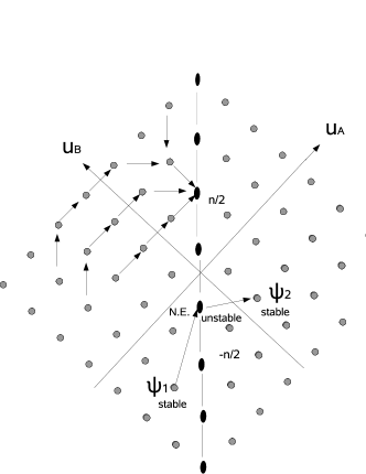
Figure 5: This is the payoff table which is rotated by $45$ degrees in clock wise direction. Each black dot represents a pair of payoff value, the elliptic black point in the middle represent the Nash-Equilibrium(N.E.) points. The game begins at an arbitrary pair of strategies, there is an imbalance between Alice’s payoff and Bob’s payoff in the begging. Then the losing player takes a better strategy to eliminate the imbalance in the next step, the winning player also choose his best response to keep his predominance. This game process is actually a renormalization group transformation, it finally converges at the Nash-Equilibrium point.

This self-characteristic vector of one player uniquely determined the probability he choose certain strategy. Thus when we introduce the mixed strategy for two players Alice and Bob,

$$|s_{A}\rangle=\sum_{k=1}^{q}\rho_{Ak}|e^{k}_{A}\rangle,\;\;\;\sum_{k}\rho_{Ak}=1,$$ (129)

$$|s_{B}\rangle=\sum_{k=1}^{p}\rho_{Bk}|e^{k}_{B}\rangle,\;\;\;\sum_{k}\rho_{Bk}=1.$$ (130)

the self-characteristic vector of Alice and Bob have been uniquely defined by $\{\rho_{Ak}\}$ and $\{\rho_{Bk}\}$. So every mixed state has an unique fixed point in the payoff matrix. In physics, payoff function or loss function corresponds to physical observables, such as Hamiltonian, angular momentum, the given mixed strategy is just the eigenfunction with the fixed point solution as the eigenvalue. We can define the density matrix using the strategy vector $|s\rangle$, $\rho=Tr(|s\rangle\langle{s}|)$. The von Neuman entropy $S(\rho(\gamma))=-Tr(\rho(\gamma)\lg{\rho(\gamma)})$ measures the entanglement between the strategy vectors.

Game theory of Hohenberg-Kohn theorem

A many electron system can be mapped into a $n$ player game, each player carries $\pm\frac{1}{2}$ spin. The ground state energy of an electronic system is completely determined by the minimization of the total energy as a functional of the density function. The external potential together with the number of electrons completely determines the Hamiltonian, these two quantities determine all properties of the ground state. Hohenberg-Kohn theorem states: the external potential $V$ is determined, within a trivial additive constant, by the electron density. This theorem insures the that there can not exist more than one external potential for any given density.

The electrons are players, the many body wave function are the strategy space. The external potential comes from external constrain. For example, in the prisoner dilemma, the police could put the two prisoners together or separate them. If the two prisoner are put together, they would conspire to remain silent so that both of spend less time in jail. If the police put them in separated rooms, they can not communicate with each other. Since they do not trust each other, they would confess. So we see external potential from police decided the behavior of the player, or in another point of view, the external potential transform the altruistic into the selfish by separating them, and transform the selfish into the altruistic by putting them together. Therefore there is only one self-characteristic vectors for a given external potential. This is Hohenberg-Kohn theorem in game theory.

V.3 Renormalization group transformation and quantum entanglement

In fact, the von Neuman entropy measures the entanglement between the self-characteristics vectors. Every self-characteristics states vector is a mixed states of altruistic and selfish. If the player is in a complex mixed states of altruistic and selfish, it is hard to predict where he ends. The Hohenberg-Kohn theorem told us the external potential uniquely determined the state vector of players, as shown in prisoner dilemma. This suggests us a possible way to operate entanglement state using external potential.

The entanglement states grows stronger and stronger following the step of renormalization group transformation. For example, in the bargain game, the seller first gave a price to see if the buyer take it. The buyer thought it too expensive, he feedback his price to the seller. Then the buyer and seller both know each other at the first step. As this bargain goes on, they know each other better and better. In other words, the entanglement between them grows stronger and stronger. When this entanglement reach a maximal point, a Nash equilibrium state is arrived. At this point, if the seller raise one penney, the buyer won’t buy it, on the other hand, if the buyer lower the price one penney, the seller will not sell his product. When the game passed over the Nash equilibrium, the entanglement decreased dramatically.

The entanglement in non-cooperative game is much stronger than the entanglement in cooperative game. In last section, we know if the self-character of players is determined, we can uniquely find an equilibrium solution. We call the altruistic player an angle player, while the selfish a devil player. The angel player who manifests goodness, purity, and selflessness, behaves like bosons. While the devil player are fermions.

The devil player do not trust each other, they most likely to betray in the game. So two devil players would try their best to bound them together and form a pair, they increase communication and cooperation to prevent his companion from betray. The entanglement between them is very strong, this entanglement would reach a maximal when the trial is around the corner.

But angle players always trust their companions. Everything they do is to increase the welfare of other players. The angel player does not need to communicate too much. They behave much like non-interacting, indistinguishable particles. So angle player is boson. An unlimited number of bosons may occupy the same state at the same time. At low temperatures, bosons can behave very differently than fermions; all the particles will tend to congregate together at the same lowest-energy state to warm each other, this is Bose-Einstein condensate.

For a given many particle system, the entanglement can be measured by the particle-particle correlation length. the longer correlation length there exist between particles, the stronger entanglement they have. we can read the entanglement out following Kadanoff block transformation. For example, in the two dimensional Ising model, the spins are players of game. They are mixed type of players between angle and devil. Their self-characteristic state vector $|\psi\rangle$ can be expanded by four entangled eigenstates of the Bell operators: $\psi^{\pm}=\frac{1}{\sqrt{2}}(|\downarrow\rangle|\uparrow\rangle\pm|\uparrow\rangle|\downarrow\rangle),\;\phi^{\pm}=\frac{1}{\sqrt{2}}(|\downarrow\rangle|\downarrow\rangle\pm|\uparrow\rangle|\uparrow\rangle).$ The density matrix, describing all the physical variables accessible to entanglement state $|\psi\rangle$, is given by $\rho=Tr(|\psi\rangle\langle\psi|)$. Then we can calculate von Neuman entropy $S^{0}(\rho(\gamma))=-Tr(\rho(\gamma)\lg{\rho(\gamma)})$ for the first order Kadanoff block transformation. Then we construct the entanglement states between two blocks and obtained the second order von Neuman entropy $S^{1}$. We can continue this renormalization group transformation, and finally derive an exact von Neuman entropy.

V.4 Topological phase in strategy space for multi-player game

We study the topological quantity in the strategy space of n-player game in this section. The total payoff function of the $n$ players could be view ed as Hamiltonian matrix.

$$\mathbb{H}=\{\hat{u}_{1},\hat{u}_{2},...,\hat{u}_{n}\}.$$ (131)

A strategy vector of the many players’s strategy space reads

$$s=\{s^{(1)}_{i},{s^{(2)}_{j}}\ldots{s^{(n)}_{k}}\},$$ (132)

$s^{(n)}_{k}$ is the $k$th strategy of the $n$th player. $\hat{u}_{n}$ maps this strategy vector into the payoff value of the $n$th player, i.e., $\hat{u}_{n}s=u_{n}$. When the Hamiltonian matrix of the payoff function operates on this vector, it produces the eigenvalues

$$\mathbb{H}\;s=\{{u}_{1},{u}_{2},...,{u}_{n}\}.$$ (133)

The players fight against each other to reduce the difference between their payoffs

$$\Delta_{1}=u_{1}-u_{2},\;\Delta_{2}=u_{2}-u_{3},\cdot\cdot,\;\Delta_{n}=u_{n}-u_{1}.$$ (134)

In a quantum system, $u_{p}$ could be interpreted as the $p$th energy level. The Nash equilibrium solution is governed by the coexistence equation

$$D({\Delta}/{s})=\{\Delta_{1},\Delta_{2},...,\Delta_{n}\}=0.$$ (135)

The war between energy levels breaks out in the degenerated eigenspace. The players take their strategy to decrease the energy gap between them. Those points at which the energy gap vanishes are the core center of vortex, they are the energy level crossing point. The $i$th player choose strategies according to other players’ strategy, thus his strategy vector is a map from the other players’s eigen-strategy to his own space $\psi_{i}(\gamma)$. In analogy with conventional Berry phase of quantum mechanics, we proposed a general topological quantity(See Appendix J). The topological phase of many players reads

$$\Omega_{i}=i\epsilon_{tj...kl}\langle\partial_{\gamma_{t}}\psi_{i}({\gamma})|\partial_{{\gamma}_{j}}\psi_{i}({\gamma})\rangle...\langle\partial_{{\gamma}_{k}}\psi_{i}({\gamma})|\partial_{{\gamma}_{l}}\psi_{i}({\gamma})\rangle.$$

$\Omega_{i}$ is actually the Riemannian curvature tensor in the strategy vector bundle. This quantity is equivalent to a topological current of the payoff functions

$$\Omega_{i}^{p}=\prod_{j\neq{i}}\delta(\Delta_{i}-\Delta_{j})d\Delta_{1}\wedge{d\Delta_{2}}\wedge\cdots{d\Delta_{n-1}}\wedge{d\Delta_{n}}.$$

From our general generalization of conventional Berry phase, the most general topological quantity is the Chern character. In this strategy vector bundle, the Chern character can be derived from the exponential map,

$$Ch(x)=Exp({d\langle\psi(\gamma)|\wedge{d|\psi(\gamma)\rangle}}).$$ (136)

These topological quantities are good candidate to measure the entanglement between different players in strategy space. One can see from Eq. (V.4), topological charges focused on the equilibrium solutions where all players get the same payoff, there is no difference among any two players. But remember these equilibrium point are isolated point, they are the center of vortex. A tiny deviation from these point would break the equilibrium.

VI game theory of many body physics

VI.1 Cooperative game and classical many body system

The particles of a physical is the players of a game. They act following the least principal, the aim of the players is to decrease the total energy. Some of them may united to form a subgroup due to local potential. Two subgroups may fuse into one when this fusion can make both of them more stable. It will be shown the many player cooperative game(see Appendix F) is just a physics system.

We consider a 3-person cooperative game $\{1,2,3\}$. We choose the payoff function of this game as the conventional Hamiltonian, the first step of the cooperative game is to find out all subgroups $\{\emptyset,1,2,3,(1,2),(1,3),(3,2),(1,2,3)\}$. The energy function maps each subgroup to a real number,

$$\varepsilon_{\emptyset}=0,\;\varepsilon_{1},\;\varepsilon_{2},\;\varepsilon_{3},\;\varepsilon_{12},\;\varepsilon_{23},\;\varepsilon_{13},\;\varepsilon_{123}.$$ (137)

This energy mapping may have various formulas. The total energy of the three particle is $E(N)=\varepsilon_{1}+\varepsilon_{2}+\varepsilon_{3}+\varepsilon_{12}+\varepsilon_{13}+\varepsilon_{23}+\varepsilon_{123}.$ The super-additivity requires $\varepsilon_{2}+\varepsilon_{3}\leq\varepsilon_{23}$. $e(23)=\varepsilon_{23}-\varepsilon_{2}-\varepsilon_{3}$ is the difference of payoffs called excess. In fact, this is a nuclear reaction in physics. In game theory, people are looking for optimal self-content energy vector of the n particles ${\varepsilon}^{\ast}$ and the excess value pair $\epsilon_{\ast}$. In the eyes of physicist, this is group expansion algorithm.

For a standard Hamiltonian system,

$$H=\sum_{i=1}^{N}\frac{1}{2}p^{2}_{i}+V(q_{1},...,q_{N}),$$ (138)

we take $N$ particles as players, their position $q_{i}$ and momentum $P^{i}$ as their strategy, the energy is the payoff. The target of this game is to find the stable ground states.

To investigate the phase transition of this game in the frame work of our topological phase transition theory, one only need to replace the output function $\hat{O}_{ut}(\gamma)$ with the Hamiltonian $H$, or any other independent integrals in the complete set $(\phi_{1}=H,\phi_{2},...,\phi_{n})$ which are in involution. The strategy vectors is taken as $\gamma=(q_{1},...,q_{N},p_{1},...,p_{N})$. Then all the conclusion on topological phase transition we obtained in the previous section holds here.

However the physical system we encountered always have a very larger number of particles, usually $N\sim 10^{23}$. It is impractical to control the position and momentum of particles. Therefore we take a different way to model the many body system. We focus on a few interaction parameters and integrate the configuration space out. For example, we choose the Hamiltonian,

$$H=\sum_{i=1}^{N}\frac{1}{2}p^{2}_{i}+\gamma^{1}V_{1}(q_{1},...,q_{N})+\gamma^{2}V_{2}(q_{1},...,q_{N})+....$$

The interaction potential relies on $n$ players above configuration space,

$$V(\vec{q})=\gamma^{1}V_{1}+\gamma^{2}V_{2}+...+\gamma^{n}V_{n}.$$ (139)

where $\{\gamma_{1},\;\gamma_{2},...,\}$ are physical parameters, and $V_{i}=V_{i}(q_{1},...,q_{N})$ is the potential functions. We integrate out all the uncontrollable position and momentum variables in the Helmoltz free energy on configuration space, then the effective output function for a finite player game is derived, $F(\gamma_{1},\gamma_{2},...)=-(2\beta)^{-1}Log(\pi/\beta)-f(\beta,\gamma_{1},\gamma_{2},...)/\beta$. with $f(\beta,\gamma_{1},\gamma_{2},...)=\frac{1}{N}Log\int{d^{N}q\;exp[-\beta{V(\vec{q},\gamma_{1},\gamma_{2},...)}]}$.

The free energy function is merely one special component of output vector field corresponding to Hamiltonian function. We can choose any output function $O_{ut}$ on the strategy manifold, and choose a arbitrary component of the compete set whose members are in involution as Hamiltonian function $\phi_{H}$, then we introduce the renormalization group transformation upon the output vector field. The basic tangent vector field $\vec{\phi}$ to characterize the topology of the extended strategy space is given by the variational principal

$$\frac{\delta^{p}[\hat{U}{O_{ut}}(\gamma_{1},\gamma_{2},...)]}{\delta{\theta}^{p}}=\frac{\int{d^{N}q{d^{N}p}\;\exp[-\beta{\phi_{H}}]}\delta^{p}[\hat{U}{O_{ut}}]}{N\int{d^{N}q{d^{N}p}\;\exp[-\beta{\phi_{H}}]}}.$$

A special subset of renormalization group transformation is Lie group $\hat{U}=e^{i\theta\hat{L}}$. Now we can apply the topological phase transition theory to study the phase transition on the strategy space extended by the interaction parameters $\gamma=(\gamma_{1},\gamma_{2},...)$. The conventional conjugate momentum and position variables have been integrated out, they are out of the set of players for the phase transition game. Of course, people can bring them in the game, in that case, the number of players is too large to manipulate, it does not tell us any practical information.

Generally a general dynamic system can be viewed as a non-cooperative game between players $\gamma_{1},\;\gamma_{2},...\;\gamma_{n}$. If we view the classical system as a cooperative game, we can divided the effective interaction parameters $\{\gamma_{1},\gamma_{2},...,\gamma_{n}\}$ into several groups $\{(\gamma_{1},\gamma_{2}),(...\gamma_{i}),...,\gamma_{n}\}$, and consider the interaction between these groups. Then we analyze their coalition, their excess value pair, their payoff, etc. We could get the most effective information about the system through the phase coexistence equation.

VI.2 Topological phase transition of quantum many body system

The topological phase transition theory in this paper aims at the most general systems, no matter they are classical physical systems or quantum physical systems, or biological system, or social system. For a quantum many body system, any output that responses corresponding to certain input can be used to detect a phase transition. The output $\hat{O}_{ut}$ could be any physical observable, such as the correction to ground state energy $\delta{E_{g}}$, the correction to thermal potential $\delta{\Omega}$, the single-particle current operator $\hat{J}=\int{d^{3}x}j$, the number density operator $<\hat{\rho}(x)>$, the spin density operator $<\hat{\sigma}(x)>$, the free energy $F$, susceptibility $\chi$, specific heat $C_{H}$, correlation length $\xi$, compressibility $\kappa_{T}$, $\cdots$, and so on. The input are any physical parameters, such as magnetic field, electric field, radiation, temperature, pressure, on-site repulsive interaction, chemical potential, density, potential, scattering length, neutral current, electron wave, probing laser beams, enzymes, …, and so forth. Our topological phase transition theory can be successfully applied to explain the quantum tunnelling of the magnetization vector in ferromagnetic nano-particlestieyan .

We take a specific model to demonstrate the application in the following. A gas of ultracold atoms in an optical lattice has provided us a very good experimental observation of superfluid-Mott-insulator phase transitiongreiner . The system is described by the Bose-Hubbard model

$$H=-J\sum_{{\langle}i,j\rangle}a_{i}^{{\dagger}}a_{j}+\frac{U}{2}\sum_{i}a_{i}^{{\dagger}}a^{{\dagger}}_{i}a_{i}a_{i}-\sum_{i}{\mu}a^{{\dagger}}_{i}a_{i},$$ (140)

where the sum in the first term of the right-hand side is restricted to nearest neighbors and $a^{{\dagger}}_{i}$ and $a_{i}$ are the creation and annihilation operators of an atom at site $i$ respectively. $J$ is the hopping parameter. $U$ corresponds to the on site repulsion between atoms, and $\mu$ is the chemical potential. This Hamiltonian admits two conflicting forces, $J$ and $U$, player $J$ drive the particles hoping from one site to another, but $U$ repulse any particles jumps to his sits, this prevent the particles from moving site by site. The quantum phase transition is governed by the two players, when the hoping player is dominated, the ultralcold atoms can easily hop in the optical lattice, this is the superfluid phase.When the on-site repulsive force is dominated, the particles is strongly repulsed by its neighbors, so it would be difficult for him to move to other house, then the ultralcold atoms have to stay at home, this is the Mott-insulator phase.

Using mean-field approaches, the ground state energy of Bose-Hubbard model can be generally expressed as the functional of $\varepsilon_{i}$, $J$ and $U$, i.e., $E_{g}=E_{g}(\varepsilon_{i},J,U).$ Following perturbation theory up to the second orderoosten , the variation of ground state energy $\delta{E_{g}}$ is

$$\delta{E_{g}}=[\frac{g}{{U}(g-1)-J}+\frac{g+1}{J-{U}g}+1],$$ (141)

From our definition of the first order phase transition, the boundary between the superfluid and the Mott insulator phases should be decided by the equation $\delta{E_{g}}=0$. We have plotted the phase diagram(FIG. 6).

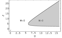
Figure 6: The phase diagram of the Bose-Hubbard Hamiltonian for g=1. Inside the curve is the Mott-insulating phase, outside the curve is the superfluid phase.

This phase diagram is in agrement with the familiar phase diagram of superfluid-Mott-insulator phase transitionoosten . It is also the same as the phase boundary obtained from the minimizing the free energychen , where they take the hopping term as perturbation.

In this phase diagram, each phase is assigned with a winding number. The winding number $\beta_{k}\eta_{k}=W_{k}$ is the generalization of the Morse index in Morse theory. Its absolute value $\beta_{k}$ measures the strength of the phase. $\eta_{k}=$sign$\{\phi^{1},\phi^{2}\}=\pm 1$, represents different phases. In the dark area circulated by the curve, $\eta_{k}=$sign$\{\phi^{1},\phi^{2}\}=+1$, it represents the Mott-Insulator phase, while outside the curve, $\eta_{k}=$sign$\{\phi^{1},\phi^{2}\}=-1$, it represents the superfluid phase. On the curve, $\{\phi^{1},\phi^{2}\}=0$, that is where a quantum phase transition takes place.

Most of the recent phase diagram of the quantum phase transition are focused on the first order. As for the $p$th-order quantum phase transition, it is characterized by a discontinuity in the $p$th derivative of the variation of ground state energy. The order parameter field of the $p$th order Quantum phase transition can be chosen as the (p-1)th derivative of $\delta{E}_{g}$ with respect to $U$ and $J$, i.e., $\phi^{1}=\partial^{p-1}_{J}\delta{E}_{g},\;\phi^{2}=\partial^{p-1}_{U}\delta{E}_{g}$. The equation of coexistence curve is given by $\{\phi^{1},\phi^{2}\}=D(\frac{\phi}{\gamma})=0$,

$$\{\phi^{1},\phi^{2}\}=\frac{\partial^{p}{\delta{E}_{g}}}{\partial{J}^{p}}\frac{\partial^{p}{\delta{E}_{g}}}{\partial{U}^{p}}-\frac{\partial\partial^{p-1}{\delta{E}_{g}}}{\partial{U}\partial{J}^{p-1}}\frac{\partial\partial^{p-1}{\delta{E}_{g}}}{\partial{J}\partial{U}^{p-1}}=0,$$ (142)

here we have taken $\gamma_{1}=U,\;\gamma_{2}=J$. From this equation, one can arrive the phase diagram of the $p$th order quantum phase transition from the equation above, and find some new quantum phases.

The above discussion is based on the correction to ground state energy, now let’s choose the output field as thermal potential, $\hat{O}_{ut}=\Delta{\Omega}$. One can do some perturbation calculation up to the second order, and derive the Green function,

$$G^{-1}(p,i\omega_{n})=\epsilon-\epsilon^{2}\sum_{\alpha}(\alpha+1)\{\frac{n_{\alpha}-n_{\alpha+1}}{i\omega_{n}-\alpha{U}+\mu}\}$$ (143)

The two parameters are $\{\mu.U\}$. The correction of the thermodynamic potential is

$$\Delta{\Omega}={\Omega}-\Omega_{0}=\frac{1}{\beta}\sum_{p,n}\ln[{-{\beta}G^{-1}(p,i\omega_{n})}].$$ (144)

The first order phase transition is given by $\Delta{\Omega}=0$. Put Eq. (143) into $\Delta{\Omega}=0$, we have $G^{-1}=-T.$ At zero temperature, $T=0$, it leads to $G^{-1}=0$. This is exactly the condition for the superfluid-mott-insulator phase transition in Ref. yuyue .

Now we see different physical observables are only different outputs, they lead to the same phase boundary.

VI.3 Elementary excitations and momentum space

One of the best merits of quantum many body theory on lattice is we do not need to consider canonical position coordination and its conjugate canonical momentum. The wave vector has only three spatial components. Although we can not manipulate them, they are very good candidates for the player of a game.

The inverse of the wave vector is wave length which is quantized due to boundaries in a finite solid state lattice. Like the string fixed at both ends, the wave vector of the standing wave modes only take a few discrete values. The standing wave patterns of the electron wave and atomic wave in lattice is viewed as elementary excitations, or quasi-particles. If we think the electrons as soldiers, the elementary excitation is the collective dancing of millions of soldiers. When the soldiers are confined in a square battlefield, they self-reorganized into certain dancing modes to avoid crashing each other. In fact, the independent spatial components of wave vector are their commanders, this is a war game between wave vectors. These oscillation modes, or elementary excitations, are the surviving strategies of the commanders in this battle.

In quantum many body system, the elementary excitations sit at the singular points of the green function. The external response can be derived from green function by linear response theory(see Appendix K). These responses are the output vector field of a quantum many body game. For the most general case, we set the Green function on a $m$ dimensional momentum space, $p\equiv(p_{0}=E,p_{1},p_{2},...,p_{m})$. In analogy the topological current of Riemannian curvature tensor on $m$ dimensional manifold, we introduce the topological current of $N$-point Green function $G$ in momentum space,

$$B_{G}=\epsilon_{tj...kl}\langle\partial_{p_{t}}G|\partial_{p_{j}}G\rangle...\langle\partial_{p_{k}}G|\partial_{p_{l}}G\rangle,$$ (145)

where we denote $|\partial_{p_{l}}G\rangle=\partial_{p_{l}}G(p)$ and $\langle\partial_{p_{k}}G|=\partial_{p_{l}}G^{{\dagger}}(p)$. The inner product between Bra $\langle|$and Ket $|\rangle$ is an integral, i.e., $\langle\partial_{p_{t}}G|\partial_{p_{j}}G\rangle=\int{dp}\partial_{p_{t}}G^{{\dagger}}_{N}(p)\partial_{p_{j}}G_{i}(p)$. Use this topological current, we can construct a more general topological action

$$Ch(M)=Tr(\exp\frac{i}{\pi}d{\langle}G(p)|\wedge{d}|G(p)\rangle).$$ (146)

This topological action measures the non-trivial topology of Green function which maps the momentum space to an external response. The Green function corresponding to the exactly solvable terms of hamiltonian can be exactly derived, the non-exactly solvable part is always calculated using perturbation theory. According to Dyson equation, the difference between the inverse of exact Green function and the exactly solvable Green function gave us the correction to energy,

$$\delta{{E}}=G(p,E)^{-1}-{G_{0}(P,E)}^{-1}=\Sigma(p,E).$$ (147)

usually people call it self-energy $\Sigma(p,E)$. In this case, the nontrivial topological current of the N-point Green function focus on

$$B_{p}=Tr[{d\langle{\Sigma}|\wedge{d|{\Sigma}\rangle}\cdots{\wedge}d\langle{\Sigma}|\wedge{d|{\Sigma}\rangle}}_{2p}],$$ (148)

again we have the holographic topological action

$$Ch(M)_{\Sigma}=Tr(\exp\frac{i}{\pi}d{\langle}{\Sigma(p,E)}|\wedge{d}|{\Sigma(p,E)}\rangle).$$ (149)

The self-energy here is the output vector field. The momentum vector and frequency are the strategies. The surviving strategies are where the stable elementary excitations arise. One may apply a Lie group transformation to self-energy to check if there the discontinuity exist. Usually we take $SO(4)$ whose element can be written as $U(\theta)=e^{\theta{\hat{L}}}=\sum_{0}^{n}\frac{1}{n!}(\hat{L}\theta)^{n},$ where $\hat{L}$ is the generator of $SO(4)$, it is operator constructed from the momentum vector $P$ and energy $E$. If there is discontinuity, we introduce the vector field $\vec{\phi}=\frac{\delta{U(\theta)\Sigma(p,E)}}{\delta\theta}$. Then we can use the phase coexistence equation $\{\phi^{i},\phi^{j},...,\phi^{k}\}=0$ to decide the phase boundary.

We always assume the periodic boundary condition in solid state physics, this boundary condition created a torus lattice manifold. This naturally leads to a topological constrain in momentum space. If we take the components of momentum as the player of a game, their strategy space is the momentum space. If the momentum space is noncompact, there is no topological constrain on strategies. If the momentum space is a compact manifold like sphere or torus, there is a nontrivial topological constrain on strategy manifold.

To avoid the non-figurative reasoning, we consider the superconducting pairing Hamiltonian schrieffer ,

$$H_{e}=\sum_{ij}(t_{ij}^{\sigma}c_{i\sigma}^{{\dagger}}c_{j\sigma}+\Delta_{ij}c^{{\dagger}}_{i\uparrow}c^{{\dagger}}_{j\downarrow}+\Delta_{ij}^{\ast}c_{j\downarrow}c_{i\uparrow})-\mu\sum_{i\sigma}c_{i\sigma}^{{\dagger}}c_{i\sigma}.$$ (150)

If the system is translationally invariant, then $t_{ij}^{\sigma}=t^{\sigma}(i-j)$ and $\Delta_{ij}=\Delta(i-j)$. We further require that hopping rate for the up-spin and down spin is the same, $t_{ij}^{\uparrow}=t_{ji}^{\downarrow}$, then the up-spin and down-spin have the same kinetic energy $\xi^{\uparrow}(k)=\xi^{\downarrow}(k)=\xi(k)=\sum_{j}e^{-ik\cdot{r_{j}}}t^{\sigma}(j)-\mu$. The momentum representation of Hamiltonian $H_{e}$ is simplified as

$$H_{e}(k)=\vec{R}(k)\cdot{\vec{\sigma}},$$ (151)

where $\vec{\sigma}=(\sigma_{x},\sigma_{y},\sigma_{z})$ are the Pauli matrices, and $\vec{R}=(R^{x},R^{y},R^{z})=[Re\Delta(k),-Im\Delta(k),\xi(k)]$ with $\Delta(k)=\sum_{j}e^{-ik\cdot{r_{j}}}\Delta(j)$ as the gap function. Using the Bogoliubov transformation, $\alpha_{k}=u_{k}c_{k}-v_{k}c_{-k}^{{\dagger}},\;\alpha_{k}^{{\dagger}}=u_{k}^{\ast}c_{k}^{{\dagger}}-v_{k}^{\ast}c_{-k}$ and considering $[\alpha_{k},H_{e}]=E_{k}\alpha_{k}$ for all $k$, the effective Hamiltonian becomes $H_{e}=\sum_{k}E_{k}\alpha_{k}^{{\dagger}}\alpha_{k}+const$ with $E_{k}\geq 0$. The effective energy of quasi-particle is $E_{k}=\sqrt{\xi_{k}^{2}+|\Delta_{k}|^{2}}.$ The Anderson’s pseudospin vectoranderson

$$\vec{n}=\frac{(Re\Delta_{k},\;-Im\Delta_{k},\;\xi_{k})}{E_{k}}.$$ (152)

The pseudospin vector $\vec{n}$ describes a mapping from k-space to a sphere $S^{2}$ in the pseudospin spacereadprb . This map defined a topological number to classify the topology of the momentum space.

As observed in the calculated results for the berry phase curvature in SrRu$O_{3}$. It has a very sharp peak near the $\Gamma$-point and ridges along the diagonalsmonom . The origin for this sharp structure is the degeneracy and band crossing. The transverse conductivity $\sigma_{xy}$ is given bythouless

$$\sigma_{xy}=\sum_{k}\frac{1}{e^{{\beta}(\varepsilon_{k}-\mu)}+1}\Omega_{xy}(k).$$ (153)

We applied the topological current theoryDuanSLAC to the momentum space of this pairing Hamiltonian, and proved that the curvature only exist at the solutions of $\vec{R}=0$, i.e.,

$$\Omega_{xy}=\sum_{k}W_{l}\delta(k^{\mu}-k^{\mu}_{l})$$ (154)

While $W_{l}$ is just the winding number of $\vec{{R}}$ around the $l$-th solution $\vec{R}(k_{l})=0$.

If we take the whole two dimensional system as a war, the soldiers are the two momentum components $\vec{k}=(p_{l},p_{2})$. Each $p_{i}$ has a strategy space which is his available value across the whole momentum space. $p_{i}$ fights against each other to steer the navigation of quasi-particle. If the whole system is homogeneous and external potential is not anisotropic, $p_{l}$ and $p_{2}$ are exchangeable. In real space, the electrons in a homogeneous system has no bias direction, they circular around each other. Two dimensional system is rather special, the electrons have to dance around each other to avoid crashing. When the external magnetic field is present, the electrons change their pattern of motion in real space, they are adjusting their wavelength and oscillation modes in the mean time. The electrons are spontaneous organized into collective oscillating modes in which any two of them form pairs.

The interference of the electron wave forms periodic distribution in the two dimensional momentum plane. Generally speaking, $p_{1}$ and $p_{2}$ are much like coworkers, they balance their inner conflicting profits to fit the environment. The best surviving strategy focused on the extremal point of the external potential, at these points, the quasi-particle or collective oscillation modes do not cost energy any more. Those solutions are given by $\vec{R}=0$. These periodically distributed extremal points are the basic channels through which the electron like to travel. Each of these channels may be view as the center of cyclone, they carry a winding number. The sum of the winding numbers of all these channels is under a topological constrain which comes form the topology of momentum manifold.

The topology of momentum manifold strongly depend on boundary condition. It seems strange for a brick of material with a rough surface to have some periodic or other boundary condition for the wave function of electrons. In fact, like the droplet of water in vacuum without gravitational field, their surface are spontaneously compact sphere. Compact boundary is one way for a system to fit the environment under certain environment. In other worlds, compact boundary condition is the result of evolution following the Principal of Least Action(The principal we talked bout here is the generalized principal of least action in the first several sections of this paper).

Therefore he electrons are organized into certain compact boundary condition by themselves in order to save energy or to form a more stable state. The topology of their momentum space is modified according to external inputs, such as chemical potential, magnetic field, et al. Anyway, if the Hamiltonian relies on many physical parameter $\{\gamma^{i},i=1,2,...\}$, i.e., $H=H(\gamma^{1},\gamma^{2},...)$, the coexisting boundary at which they reach a balance is given by

$$D(\hat{\phi}/{\gamma})=[\hat{\phi}_{1},\hat{\phi}_{2},...,\hat{\phi}_{n}]=0.$$ (155)

If one of the operator is taken as Hamiltonian itself, $\hat{\phi}=\hat{H}$, this is nothing but the complete set of dynamic system in parameter space.

VI.4 Quantum many body theory of game

The player of war consists of a large number of soldiers which act like identical particles. The soldiers split into several subgroups, inside every subgroup there is a common agreement constituted and obeyed by all the members of the association. Thus we may take mean field approach inside the subgroup whose member move in a mean-field potential formed by all the other members.

Generally speaking, the subgroup consists of angel players is stronger than that of devil players. Angle players are bosonic players. The collective strategy is the symmetric combination of the personal strategy,

$$|S_{Bos}(1,2,...,n)\rangle=\sqrt{\frac{\prod{m!}}{n!}}P(|s^{(1)}\rangle|s^{(2)}\rangle....|s^{(n)}\rangle).$$

The devil payer are fermionic players. Their collective strategy is a totally anti-symmetric strategy, which can be written as Slater determinant,

$$|S_{Fer}\rangle=\sum\frac{1}{n!}\varepsilon_{ij...k}\varepsilon^{\alpha_{1}\alpha_{2}...\alpha_{n}}(|s_{\alpha_{1}}^{(i)}\rangle|s_{\alpha_{2}}^{(j)}\rangle....|s_{\alpha_{n}}^{(n)}\rangle).$$

The above discussion is only suitable for some oversimplified system. When it comes to a general multi player game, we do not distinguish which one is angel player and which one is devil player. They are all rational players. In every round of the game, the player choose one strategy from his strategy space, so do other players. When they check their payoffs, what someone win is what someone lose. We may call the individual loser an angel player, and call the individual winner a devil player.

In fact, the players share the same strategy space. A wining player takes good strategies, a losing player takes those bad ones. It does not make any sense to talk about the good or the bad of the strategy itself, the same strategy may bring different results in different situations for a certain layer. Every combinatorial series of strategies corresponds to a payoff distribution to individual players. If we take particles as player, a physics system always contain millions of particles, it is impossible to calculate every particle’s payoff. That is why we need statistics physics through which we summarize the information of payoffs into a few statistical observables, but we lost the information on individual payoffs. We choose a more practical way to grab the key information of many particle system. The player of game is taken as the different interactions that govern the microscopic behavior of particle.

A vacuum state $|0\rangle$ is defined by a state that no player confirm his strategy. When the $i$th player has chosen his strategy $|s_{\alpha_{1}}^{(i)}\rangle$, and place his card on the table, it means that a strategy $s_{\alpha}$ is generated from vacuum, i.e., $|s_{\alpha}^{(i)}\rangle=\hat{s}_{i\alpha}^{{\dagger}}|0\rangle$. One player’s strategy is not isolated, it is always entangled with other players’s strategy, since whenever he makes the decision he must reflects other player’s choice, the collective strategy is highly entangled states. The anti-strategy of the $i$th player comes from the combination strategy he received from the rest players, we denote it as

$$\langle{S}^{i}|=\langle 0|\hat{F}(\hat{s}_{\alpha_{1}},\hat{s}_{\alpha_{2}},...,\hat{s}_{\alpha_{k}},...\hat{s}_{\alpha_{n}}),\;(k\neq{i}).$$

When the $i$th player encounter the $j$th player, his payoff is $u_{ij}=Tr_{k\neq{j}}[\langle{S}^{i}|s_{\alpha}^{(i)}\rangle]$. We can further define the density matrix $\rho=\sum_{j}p_{j}|S_{j}\rangle\langle{S}_{j}|$, and introduce the familiar Von Neumann entropy to measure the entanglement.

Pairing mechanism in the war game

As shown in the prisoner dilemma, two altruistic players can get their best payoff without communication and cooperate, they trust each other and both choose the strategy for the welfare of other people. But two selfish player can not get the best payoffs unless they communicate and cooperate, in order to prevent the other player’s betray, they would like to bound into a pair so that any betray would damage himself, this increases the entanglement between them. in physics, two spin in magnetic field is a perfect physical system to realize a prisoner dilemma. A direct physical observation is that the particles with spin is lean to form pairs, and the magnetic field would strengthen the entanglement between two particles with opposite spins.

Figure 7: Two spins in magnetic field is a good demonstration of prisoner dilemma in physics.

A physical system to demonstrate the Prisoner’s dilemma is two spins in magnetic field. Two players are the two particles: Alice and Bob, they both carry magnetic dipole momentum $\mu$. The strategies: confession and accusation corresponds to spin up and spin down, the external magnetic field is external law. Their loss function is their energy in this system. They fight to minimize their loss function. The payoff matrix is

Bob Bob

  $$\downarrow$$   

Alice   

Alice   

$\Delta$ is the energy shift due to the interaction between the two particles. This is the classical picture of two-particle game. There was experimental realization of prisoner dilemma on nuclear magnetic resonance quantum computer jfdu .

A general $n$-player prisoner dilemma may be summarized into a $n$-spin Hamiltonian. A player has two strategies: spin-up and spin-down. The payoff function is the Hamiltonian,

$$H=\sum_{i}h_{i}\sigma_{z}^{i}+J^{ij}\sum_{ij}\sigma_{z}^{i}\sigma_{z}^{j}.$$ (156)

If we take the local coupling $J^{ij}=J$ and consider only the nearest neighbor interaction, this Hamiltonian becomes traditional Ising model. The payoff matrix of this $n$-player prisoner dilemma game for Ising model is diagonal block. A group of soldiers in a war also encounter prisoner dilemma. Two soldiers helping each other is stronger than the two that they do not help each other.

We consider a war on two dimensional lattice. The soldiers are particles, they are divided into two equal groups, ${A}$ and ${B}$. The particles of $A$ is the anti-particle of $B$ and vice versa. In the beginning, $A$ and $B$ are separated two parts on the lattice. When the war break out, they rush to each other and began the combat. A particle only fight against his nearest antiparticles and help his nearest friend neighbors. If the soldiers are identical particles at the same level, the interaction between particles does not go too far, it is confined in a local region. If we assume all the soldiers only fight against enemy soldiers for his own survival, they do help friend neighbors, the dynamic process only includes

$$\{\varepsilon_{ij}\;\hat{s}_{A_{i}}^{{\dagger}}\hat{s}_{B_{j}},\;\;\;\varepsilon_{ji}\;\hat{s}_{B_{j}}^{{\dagger}}\hat{s}_{A_{i}},\;\;\;A_{i}\in{A},B_{j}\in{{\bar{B}}}\},$$ (157)

where $s$ represents the soldiers. This is a system composed of free particle and antiparticles. In fact, some soldiers of $G$ may help each other, they grouped into pairs to fight. So does the soldiers of ${\bar{G}}$. Then we have to consider the pair interactions. The war now contains three solders interaction and four soldiers interaction,

$$\varepsilon_{ij}\;\hat{s}_{A_{i}}^{{\dagger}}\hat{s}_{B_{j}},\;\;\;\varepsilon_{ji}\;\hat{s}_{B_{j}}^{{\dagger}}\hat{s}_{A_{i}},$$

$$V^{3}\;\hat{s}_{A_{i}}^{{\dagger}}\hat{s}_{A_{k}}^{{\dagger}}\hat{s}_{B_{j}},\;...\;\;,\varepsilon_{ji}\;\hat{s}_{B_{j}}^{{\dagger}}\hat{s}_{B_{k}}^{{\dagger}}\hat{s}_{A_{i}},$$

$$V^{4}\;\hat{s}_{{A_{i}}}^{{\dagger}}\hat{s}_{{A_{j}}}^{{\dagger}}\hat{s}_{{B_{k}}}\hat{s}_{{B_{l}}},\;\;V^{4}\;\hat{s}_{{B_{i}}}^{{\dagger}}\hat{s}_{{B_{j}}}^{{\dagger}}\hat{s}_{{A_{k}}}\hat{s}_{{A_{l}}}.$$

If we recall the BCS pairing mechanism in superconductor theory, the war between electrons does not have three-particle interaction. Even two electrons separated far from each other, they can act as one pair. They do not even know each other, since identical particle are indistinguishable. This interesting phenomena in the quantum world may found some naive analogy in war. During the war game, we can assume a pair of soldier are confined in the lattice, they kept running from one place to anther, but helping each other all the time. They shot any enemy that try to kill his partner. This is a long range interaction.

There are two types of pairs, angle pair and devil pair. The angle pair is more powerful than the devil pair as a whole. They love each other and trust each other, so they can separated from each other in a longer distance. But devil player have to stay closer to prevent his partner from betraying him for his own survival, their correlation length is shorter.

There are hierarchical structure in army. The soldiers are organized into different groups in which a large number of them fight as a whole. These hierarchical structure are well kept in the region far from the coexistence boundary, but when combat begins in one battlefield, all these hierarchical structure becomes meaningless, the general or the captain at high plays no different role as an ordinary soldier at the lowest level, they are just the same individual fighters with arm. It is the hierarchical structure or inner structure of a system that differs it from others. When the phase transition occurs, all these hierarchical structure are broken, men are born to equal, men are also died to equal. This is the origin of universality class.

For a further consideration of war game, we have to take into count of different hierarchical structures. The commanders are the critical players, they are dressed up by a group soldiers, and fight as a whole around the battlefield. We may take Kadanoff block procedure to summarize all the many player interaction to the commander. The many body interactions, such as

$$V^{n}\;\hat{s}_{{B_{i}}}^{{\dagger}}\;...\;\hat{s}_{{B_{j}}}^{{\dagger}}\;...\;\hat{s}_{{A_{k}}}\;...\;\hat{s}_{{A_{l}}},\\$$

are renormalized into partition function. The war is going on between the renormalized commanders, ${S}_{B}$ and ${S}_{A}$, where

$$(\hat{s}_{{B_{i}}}^{{\dagger}}\;...\;\hat{s}_{{B_{j}}}^{{\dagger}})\rightarrow{\hat{S}}_{B},\;\;(\hat{s}_{{A_{i}}}^{{\dagger}}\;...\;\hat{s}_{{A_{j}}}^{{\dagger}})\rightarrow{\hat{S}}_{A}.$$ (159)

Again we may consider the pairing interactions among these commanders,

$$V^{3}_{S}\;\hat{S}_{A_{i}}^{{\dagger}}\hat{S}_{A_{k}}^{{\dagger}}\hat{S}_{B_{j}},\;...\;\;,\varepsilon_{ji}\;\hat{S}_{B_{j}}^{{\dagger}}\hat{S}_{B_{k}}^{{\dagger}}\hat{S}_{A_{i}},$$

$$V^{4}_{S}\;\hat{S}_{{A_{i}}}^{{\dagger}}\hat{S}_{{A_{j}}}^{{\dagger}}\hat{S}_{{B_{k}}}\hat{S}_{{B_{l}}},\;\;V^{4}\;\hat{S}_{{B_{i}}}^{{\dagger}}\hat{S}_{{B_{j}}}^{{\dagger}}\hat{S}_{{A_{k}}}\hat{S}_{{A_{l}}}.$$

Repeating this renormalization group transformation, we transform the sophisticate many body problems into something we can handle. This is the fundamental spirit of various numerical renormalization group method developed in quantum many body system.

The phase boundary appears when the fighting groups reach a balance at certain frontiers regions. Friend and enemy are maximally entangled in the coexistence state. One can not tell who is who. In order to study the symmetry transformation at the coexistence boundary, we introduce the position displacement operator and its conjugate momentum operator,

$$X_{j}=\frac{\hat{S}_{j}^{{\dagger}}+\hat{S}_{j}}{\sqrt{2}},\;\;\;P_{j}=\frac{i(\hat{S}_{j}^{{\dagger}}-\hat{S}_{j})}{\sqrt{2}}.$$ (161)

Then the angular momentum operator is given by $L_{ij}=(X_{i}P_{j}-X_{j}P_{i})$. The generator of the symmetry transformation may be denoted as $\hat{L}={i\sum_{ij}\theta{L}_{ij}}$, through which we derived the Lie group element

$$U=e^{i\theta\hat{L}}=e^{{-i\sum_{ij}\theta(\hat{S}_{i}^{{\dagger}}\hat{S}_{j}^{{\dagger}}-\hat{S}_{i}\hat{S}_{j})}}.$$ (162)

The quantum output vector $\hat{O}_{ut}(\hat{S}_{i},\hat{S}_{j},...)$ is expressed by the operator of renormalized soldiers. Then we can detect the phase transition by the transformation

$$U_{(p)}\hat{O}_{ut}{U}_{(p)}^{-1}=e^{i\theta\cdot{\hat{L}}}\hat{O}_{ut}e^{-i\theta\cdot{\hat{L}}}$$ (163)

This transformation equation determined the evolution of the quantum output in the vicinity of phase coexistence region. Inside one phase, or inside one army, this transformation is continuous up to infinite order. When never the symmetry lost, an enemy popped out and initiated the revolution.

The uncertainty principal shows up across the whole phase diagram. In the phase diagram, the war game is in different squeeze state for different stage of combat. The transformation operator (162) is a special squeeze operator. A general squeeze statescully generated from vacuum is

$$|\psi\rangle=e^{{-i\sum_{ij}(\theta\hat{S}_{i}^{{\dagger}}\hat{S}_{j}^{{\dagger}}-\theta^{\ast}\hat{S}_{i}\hat{S}_{j})}}|0\rangle.$$ (164)

When the two players began rushing toward each other but still do not touch each other, their fluctuation of spacial position is much higher than that of their force. When they meet in the phase coexistence boundary, the fluctuation of spatial position is around the boundary, it is much lower than the conflicting force. At the Nash equilibrium state, the phase boundary is almost stationary, but both of the two players summon up their maximal force to against each other, they reach a dangerous equilibrium state on the boundary. This is an extremal squeezed state, the fluctuation of position is highly squeezed, but the fluctuation of conflicting force is very strong.

So we may take two Hermitian operators $\gamma$ and $P_{\gamma}$, $\gamma$ denotes the position in phase diagram, $P_{\gamma}$ represents the corresponding force. The commutation relation derive from the second quantization is $[\gamma,P_{\gamma}]=iC$. We can calculate the uncertainty of an operator $A$ by $(\Delta{A})^{2}={\langle\psi|A^{2}|\psi\rangle-(\langle\psi|A|\psi\rangle)^{2}}$. According to Heisenberg uncertainty principal, $\Delta{\gamma}\Delta{P_{\gamma}}\geq\frac{1}{2}|C|$. The uncertainty of the position operator is

$$\Delta{\gamma}\ll\frac{1}{2}|C|$$ (165)

at the coexistence state. While the uncertainty of corresponding momentum is much stronger $\Delta{P_{\gamma}}\gg\frac{1}{2}|C|$.

The angel pairing and devil pairing are two stable squeezed states. The angle pairing has less uncertainty about their trustworthiness, so they have larger uncertainty on their spatial connection. But the devil pair has larger uncertainty on his partner’s trustworthiness, so they strengthen their spatial connection, this reduced their spatial uncertainty. No matter which kind of pairing it is, the total information in the two pairing states should be conserved. If we can make sure a system doe not lose information, we can maintain the pairing to a stable level. Superconductor is such a system, below the critical temperature, no chaos invades into it, no information escapes out of it. There is a constant electric flow.

According to quantum field theory, symmetry means conserved quantity, a loss of symmetry indicates a loss of conserved quantity. What the old phase lost becomes the generator of the new phase. The squeeze transformation on output field is a way to detect the loss of information. Imbalance is the original engine of development. For physicist, the physical measurement always affect the output state itself. We can not detect a state without changing it, this minor change is neglectable when it is done in a stable phase. But at critical region, the minor effect of detection might induce significant effect. In other words, when a war is going on, once the spy step into the frontier, he is force to fight for his own survival, it would be too hard for him to sent out any information.

VII summary

(1)game theory of general phase transition and  Renormaization group transformation

Phase transition is a much more universal phenomena than the conventional phase transitions in physics. Similar sudden changes arise from evolution of biomolecule, self-organization in nanoscale systems, cosmic evolution, and so forth. The general phase transition breaking the envelop of physics can be viewed as a non-cooperative game of many players. The players try different strategies to win. Whenever a winning player fails and becomes a loser, a phase transition would occur.

When the players represent different interactions between the elements of a complex system, a winning player is a dominant interaction which governs one stable phase of the system, the other phases represented by loser’s interaction are suppressed. When we tune the interaction parameters, we are changing the strategies of the players, the winning interaction may becomes weaker and weaker. There is a critical point at which the losing players grows stronger enough to balance the previous winning player, then we arrived the Nash equilibrium point. At this point , no one wins, and no one losses, it is the coexistence point of the new phase and old phase. The Nash equilibrium point is an unstable saddle point, any tiny deviation would decided the fate of the coexisting new phase and old phase, there is only one winner left to dominate the phase structure of the system.

Usually the Nash equilibrium of a war game is not derived in one round of combat. The players have to play many rounds of negotiation to find the optimal strategy. The renormalization group transformation theory is actually one theoretical description of this kind of game process in physics. In physics, the players are the interaction parameter or physical parameter. For example, we take the Ising model as a game, the two players are the spin coupling interaction and external magnetic field. The stable phase is determined by the dominant interaction.

At the first round of renormalization group transformation, the two player accomplished the first round of combat, they made an agreement on the most part of boundary between their domains. But the unsettled part is occupied by the winner. So the loser initiated the second round of renormalization group transformation to get some of his losing back. As this transformation goes on, the unsettled boundary between the players becomes less and less. Finally, they reach the Nash equilibrium point, that is the fixed point of the renormalization group transformation. This point is where the phase transition occurs.

Usually to obtain the exact critical point, one has to perform the renormalization group transformation to infinite order. However, it is too far to reach in reality, we always cut it off at certain order. It inevitably gives birth to a loser and a winner to certain order. Although the players at that order maybe are fighting for only one thousandth of a penny, but the loser is loser, winner is winner, the title is fixed. The order of cutoff is the order of phase transition. we can take renormalization group transformation on output function to observe different order of phase transition. When we apply this definition to thermodynamics physics, it naturally unified Ehrenfest definition.

(2)Universal coexistence equation and topological conjecture of scaling laws in fractal space

The game is played on the strategy base manifold, so a phase transition is related to the topology of the strategy base manifold. If the strategy space is noncompact, we do not need to consider topology at all, in that cases, the phase transition governed by game dynamics. We may call it a non-topological phase transition. When the strategy manifold is compact, there would be a topological constrain on the player’s strategies, then the topological effect would appear in phase transition, we call it a topological phase transition.

The topology is intimately related to the fixed points of renormalization group transformation flow on strategy manifold. We introduced the general flow vector field, and showed that the sum of the winding number around the surviving strategies is a topological number. These surviving strategies with opposite charges annihilate at the universal coexistence curve, whose equation is $\{\phi^{1},\phi^{2},...,\phi^{2}\}=0$, $\phi^{i}$ are the component of the flow vector field of output field. In the thermodynamics physics, the output field may be chosen as free energy, the players are temperature and pressure, one can verify that this coexistence equation unified all the coexistence equations at different order classical phase transition. The phases separated by the coexistence curve are assigned with different winding number of opposite sign.

The strategy space is a fractal dimensional space. It is easy to see this point from a war game. We focus on the battlefield, it is a war between two armies. If we look closer, it is the war between corps. We may continue the magnify the battle field, one would see, it is a war at all different scales, it is the combat between two individual soldiers at any local region. A war game may be summarized into the war between two commanders by Kadanoff-block procedure. There is an intrinsic fractal structure around the critical point. So we make the hypothesis that a local neighborhood on the strategy base manifold is homeomorphic to a fractal dimensional space. Then the output field may be expanded by the polynomial of power functions with fractal dimension index. In analogy with the observables defined in the statistical mechanics, we introduce the tangent vector field of the output field as observables. These tangent vector field may be approximated by fractal polynomials in the vicinity of Nash equilibrium solution. By substituting these fractal polynomials into the universal coexistence equation, one can derive the scaling relations. As we shown, the coexistence operator has a degenerated subspace, the coexistence equation bear a topological origin, so these scaling relations are universal.

(3)Many body physics of games

Game theory is actually one different way to see many body system. For example, a collection of millions of ultralcold atoms trapped in optical lattice can be described by Bose-Hubbard model. There are two key parameter, the hopping parameter $J$ and the on site repulsive interaction $U$. We can model this system as a game between $U$ and $J$. Player $J$ command the particles hoping from one site to another, drive them into superfluid phase. While $U$ direct the soldiers to stick to the lattice site. If $J$ wins, the ultracold atoms becomes superfluid. If $U$ wins, the ultracold atoms are confined in the lattice, they form Mott-insulator phase. The transition point is the Nash equilibrium point of this game. The two phases coexist at the critical point. Another way to model the millions of ultracold atoms is to take every atom as a player, and their states at lattice sites are strategy space, this reproduced the standard quantum many body theory.

A practical approach to a given many body system is first to find out the main different interactions that are players of the game. Secondly, we choose some output quantity to measure the states. Physicist usually take the external response function, these output field are the payoff function of the game. The tangent vector field established on the hypersurface of these response function is the fundamental vector field to study the topological effect of the strategy space. Applying the universal coexistence equation, we can find out the basic structure of different phases. This scheme holds both for classical systems and quantum systems.

Game theory only provide us a mathematical frame work to understanding the general property of a system. The topological phase transition theory developed in this paper is a general mathematical results, it does not depend on any specific model in physics, biology or social system. When it comes to some specific physical system, we may apply the conventional theory for that special system to derive the specific relation between input parameters and output field, or one may directly conduct some experiments to find some approximated relation. As long as one derived the specific relation between output and input, just substitute it into the universal coexistence equation, one can get basic phase diagram.

In fact, quantum many body theory may provide us new understanding to many player games. We developed the density matrix theory of many player game, it was shown there is a one-to-one correspondence between fixed point of many player game and the self-character vector of the player. Every quantum phase may be represented by a state function, these state functions are the players of multi-player game. A player’s strategy must take into account of the other players’s strategy. So game theory is born to be an entangled theory. This may help us to understand the entanglement among coexistence phases. We find a new quantity to measure the entanglement of different phases. The maximal point of entanglement is the Nash equilibrium point at which different phases coexist. The maximal entanglement between phases is controlled by interaction parameter instead of time, so the quantum entanglement between different quantum phases are good candidates for quantum computation.

Further more, if we take two particles as the two players of prisoner dilemma, it would be found that there are two types of entangled pairs: the angel pair and devil pair, the angel pair love each other, their entanglement is a little bit weaker. While the devil players do not trust each other, they inclined to bounded together to prevent the other from betray, it is a strong entangled pair. This may help us to understand pairing mechanism in superconductor.

VIII Acknowledgment

The author expresses his gratitude to professor Yue Yu for his support. This work was supported by the National Natural Science Foundation of China.

Appendix A Ehrenfest’s definition about order of phase transition

The zeroth order phase transition defines that the free energy of the two phases $F(T,P)$ are not equal,

$$F_{A}(T,P){\neq}F_{B}(T,P).$$ (166)

For the first order phase transition, the free energy of the two phases $F_{A}$ and $F_{B}$ is continuous, but the first order derivative is not continuous,

$$F_{A}(T,P)=F_{B}(T,P),\;\;\;\frac{dF_{A}}{dT}\neq\frac{dF_{B}}{dT},\;\;\frac{dF_{A}}{dP}\neq\frac{dF_{B}}{dP}.$$ (167)

The second order phase transition is defined by the discontinuity of the compressibility, susceptibility,

$$C_{p}^{A}\neq{C_{p}^{B}},\;\;\alpha^{A}\neq\alpha^{B},\;\;\kappa^{A}\neq\kappa^{B},$$ (168)

in which the specific heat $C_{p}$, $\alpha,\kappa$ are defined as:

$$C_{p}=T(\frac{dS}{dT})_{P}=-T\frac{\partial^{2}F}{dT^{2}},$$

$$\alpha=\frac{1}{V}(\frac{\partial{V}}{\partial{T}})_{P}=\frac{1}{V}\frac{\partial^{2}F}{\partial{T}\partial{P}},$$

$$\kappa=-\frac{1}{V}(\frac{\partial{V}}{\partial{P}})_{P}=-\frac{1}{V}\frac{\partial^{2}F}{\partial{P}^{2}}.$$ (169)

The higher order of phase transition is defined from the discontinuity of higher order derivative of free energy. We rewrite Ehrenfest’s definition into more compact formulism. The $p$th-order quantum phase transition is characterized by a discontinuity in the $p$th derivative of difference of free energy $\delta{F}$,

$$\partial^{p-1}_{\gamma_{1}}\delta{F=0},\;\;\partial^{m}_{\gamma_{1}}\partial^{p-m-1}_{\gamma_{2}}\delta{F=0},(m=1,2,...,p-1),$$

$$\partial^{p-1}_{\gamma_{2}}\delta{F=0}.$$

$$\partial^{p}_{\gamma_{1}}\delta{F\neq 0},\;\;\partial^{m}_{\gamma_{1}}\partial^{p-m}_{\gamma_{2}}\delta{F\neq 0},(m=1,2,...,p),$$

$$\partial^{p}_{\gamma_{2}}\delta{F\neq 0}.$$ (170)

If the $p$th derivative of $\delta{F}$ becomes continuous, the phase transition jumps to the $p+1$th order.

Appendix B Differential geometry of free energy

We demonstrate the basic conception of differential geometry on the free energy manifold expanded by two thermal variables temperature $T$ and pressure $P$.

In differential geometry, the open set $\delta{F}(T,P)$ in a manifold may be mapped to an open set in three dimensional Euclidean space through the homeomorphic mapping $f_{\delta{F}}:\delta{F}(T,P)\rightarrow\textbf{X}_{\delta{F}}$, $\textbf{{X}}=X_{1}(\gamma_{1},\gamma_{2})i+X_{2}(\gamma_{1},\gamma_{2})j+X_{3}(\gamma_{1},\gamma_{2})k$, At each point $\gamma^{0}$ in $\delta{F}$ there exist a set of tangent vectors. The two basis of the tangent vector space on this manifold are

$$e_{1}=\frac{\partial}{\partial{\gamma_{1}}}=\frac{\partial}{\partial{T}},\;\;\;\;e_{2}=\frac{\partial}{\partial{\gamma_{2}}}=\frac{\partial}{\partial{T}},$$ (171)

here we have defined $\gamma_{1}=T$(temperature) and $\gamma_{1}=P$(pressure). An arbitrary tangent vectors may be expressed as

$${\textbf{X}}_{\gamma_{i}}=\frac{\partial{\textbf{{X}}}}{\partial{\gamma_{i}}},\;\;{\textbf{X}}_{\gamma_{i}\gamma_{j}}=\frac{\partial^{2}\textbf{{X}}}{\partial{\gamma_{i}}\partial{\gamma_{j}}}$$ (172)

All the tangent vectors to the surface $\delta{F}$ at x denoted form a tangent vector space denoted by $T_{x}\delta{F}$, it is parallel to the tangent plane to $\delta{F}$ at x.

The metric tensor is given in a bilinear form by the inner product of two basis vectors, $g_{ij}=<e_{i},e_{j}>$. Then the first fundamental form is

$$E={\textbf{X}}_{\gamma_{1}}\cdot{\textbf{X}}_{\gamma_{1}},\;\;\;F^{\prime}={\textbf{X}}_{\gamma_{1}}\cdot{\textbf{X}}_{\gamma_{2}},\;\;G={\textbf{X}}_{\gamma_{2}}\cdot{\textbf{X}}_{\gamma_{2}},$$

$$g_{11}=E,\;\;\;g_{12}=g_{21}=F^{\prime},\;\;\;g_{22}=G.$$ (173)

The second fundamental form is

$$L={\textbf{X}}_{\gamma_{1}\gamma_{1}}\cdot{\textbf{n}}=-{\textbf{X}}_{\gamma_{1}}\cdot{\textbf{n}_{\gamma_{1}}}$$

$$M={\textbf{X}}_{\gamma_{1}\gamma_{2}}\cdot{\textbf{n}}=-{\textbf{X}}_{\gamma_{1}}\cdot{\textbf{n}_{\gamma_{2}}}$$

$$N={\textbf{X}}_{\gamma_{2}\gamma_{2}}\cdot{\textbf{n}}=-{\textbf{X}}_{\gamma_{2}}\cdot{\textbf{n}_{\gamma_{2}}}.$$ (174)

with n as the normal vector of the surface,

$$\textbf{n}=\frac{{\textbf{X}}_{\gamma_{1}}\times{\textbf{X}}_{\gamma_{1}}}{|{\textbf{X}}_{\gamma_{1}}\times{\textbf{X}}_{\gamma_{1}}|}.$$ (175)

Considering the second order of phase transition, the first fundamental form and the second fundamental form includes more information about the variation of the free energy than Ehrenfest’s definition. It is more reasonable to choose the Gaussian curvature,

$$\Omega=\frac{LN-M^{2}}{EG-{F^{\prime}}^{2}},$$ (176)

It is positive for spheres, negative for one sheet hyperbolic surface and zero for planes. The principal curvatures, $\kappa_{1}(\gamma^{0})$ and $\kappa_{2}(\gamma^{0})$, of X at ${\textbf{X}(\gamma^{0})}$ are defined as the maximum and the minimum normal curvatures at ${\textbf{X}(\gamma^{0})}$, respectively. The directions of the tangents of the two curves that are the result of the intersection of the surface ${\textbf{X}(\gamma^{0})}$ and the planes containing ${\textbf{n}(\gamma^{0})}$. Then

$$\Omega({\gamma_{1},\gamma_{2}})=\sum_{p}\Omega({\gamma_{1},\gamma_{2}})|_{p}=\sum_{p}\kappa_{1}({\gamma_{1},\gamma_{2}})\kappa_{2}({\gamma_{1},\gamma_{2}})|_{p}.$$ (177)

The cross section of the curvature X at $\gamma^{0}$ may be expanded as parabola by ignoring the higher order,

$$X=\frac{\kappa_{1}}{2}r_{1}^{2}+\frac{\kappa_{2}}{2}r_{2}^{2}.$$ (178)

where $r_{i}=(d\gamma_{1}+\frac{1}{2}\Gamma_{ij}^{1}d\gamma_{i}d\gamma_{j})\sqrt{g_{ii}}+\cdots$. When $\kappa_{1}>0$ and $\kappa_{2}>0$, it is a elliptic surface, when $\kappa_{1}>0$ and $\kappa_{2}=0$, it is parabolic, for $\kappa_{1}>0$ and $\kappa_{2}<0$, it is hyperbolic.

The covariant derivative may be defined as

$$D_{\gamma_{i}}\phi^{j}=\partial_{\gamma_{i}}\phi^{a}+\Gamma_{ik}^{j}\phi^{k},$$ (179)

here we have introduced the Christoffel-Levi-Civita connection $\Gamma_{ij}^{k}$, which is defined as

$$\Gamma_{ij}^{k}=\frac{1}{2}g^{kl}(\frac{\partial{g_{il}}}{\partial\gamma_{j}}+\frac{\partial{g_{jl}}}{\partial\gamma_{i}}+\frac{\partial{g_{ij}}}{\partial\gamma_{l}}).$$ (180)

Appendix C Definition of game theory

A game is an abstract formulation of an interactive decision situation with possibly conflicting interests, it involves of a number of agents or players, who are allowed a certain set of moves or actions. The payoff function specifies how the players will be rewarded after they have performed their actions. Let $n=1,\ldots,N$ denote the players; The $i$th player’s strategy, $S_{i}$, is her procedure for deciding which action to play, depending on her information. The strategy space of the $i$th player $\mathcal{S}_{i}$=$\{e_{i1},e_{i2},\ldots,e_{im}\}$ is the set of strategies available to her. A strategy profile $(s_{1},s_{2},\ldots,s_{N})$ is an assignment of one strategy to each player. $u_{i}(s_{1},\ldots,s_{N})$ is player $i$’s payoff function (utility function), i.e., the measure of her satisfaction if the strategy profile $(s_{1},\ldots,s_{N})$ gets realized.

The strategy assigned to each player could be pure state or mixed state. A mixed strategy is a probability distribution over pure strategies. Playing a mixed strategy means, the players come up with one of her feasible actions with a pre-assigned probability. Each mixed strategy corresponds to a point P of the mixed strategy simplex.

$$M_{\textbf{p}}=\{\textbf{P}=(p_{1},\ldots,p_{m})\in{\mathbb{R}^{m}}:p_{q}\geq 0,\sum_{q=1}^{m}p_{q}=1\},$$ (181)

whose corners are the pure strategies. For the case of two players, a strategy profile is a pair of probability vector $(\textbf{p},\textbf{q})$ with $\textbf{p}\in{M_{\textbf{p}}}$ and $\textbf{q}\in{M_{\textbf{q}}}$. The expected payoffs of player 1 and 2 are expressed as

$$u_{1}(\textbf{p},\textbf{q})=\textbf{p}\cdot{\textbf{A}}\textbf{q}={\sum^{m}_{ij}}p_{i}A_{ij}q_{j},$$ (182)

$$u_{2}(\textbf{p},\textbf{q})=\textbf{p}\cdot{\textbf{B}}\textbf{q}={\sum^{m}_{ij}}p_{i}B_{ij}q_{j}.$$ (183)

This payoffs function relies on the entangled strategies of the two players.

The essence of a game is the payoff function defined over different strategy profile of the players. In the language of quantum statistics, the strategy space of the $i$th player $S_{A}$ is the Hilbert space of the $i$ particle.

Appendix D Differential game

The differential game is applied to model dynamic conflictslewin , such as the labor-employers relations in economic processes, the bull and fighter in bull-fighting. The labor and employer are called players in differential game. We take the two player game as an example. There are two players, one is called Alice, the other player is Bob. Alice has a strategy space ${S}_{A}(s_{1},s_{2},\ldots,s_{N})$, and Bob’s strategy space is ${S}_{B}$. We introduce the state vector $\vec{x}$ which characterize the conflict to convert a real life conflict to a differential game model. For example, Alice and Bob are concerned with the motion of a point in a plane, the state vector denotes the location of the point $x(t)$ at the time t. All possible state vector is a subset of a $n$-dimensional Euclidean space.

The influence of the decisions of the evolution of the state is described by the equations of motion,

$$\dot{x}=f(\textbf{{x}},\textbf{{s}}_{A},\textbf{{s}}_{B}).$$ (184)

When the two players realize their strategy $(\textbf{{s}}_{A},\textbf{{s}}_{B})$ at time $t$, the outcome of the differential game is functional on the state space, $U[\textbf{{x}},\textbf{{s}}_{A},\textbf{{s}}_{B}]$. If the outcome satisfies for a pair of strategy $(\textbf{{s}}^{\ast}_{A},\textbf{{s}}^{\ast}_{B})$ satisfies,

$$U[\textbf{{x}},\textbf{{s}}^{\ast}_{A},\textbf{{s}}^{\ast}_{B}]\leq{U[\textbf{{x}},\textbf{{s}}^{\ast}_{A},\textbf{{s}}^{\ast}_{B}]}\leq{U[\textbf{{x}},\textbf{{s}}_{A},\textbf{{s}}^{\ast}_{B}]},$$ (185)

then this strategy pair is the optimal play for the two players, ${U[\textbf{{x}},\textbf{{s}}^{\ast}_{A},\textbf{{s}}^{\ast}_{B}]}$ is called the optimal outcome at x. The optimal outcome is a function in the Euclidean space, it is called the value function,

$$J(\textbf{{x}})={U[\textbf{{x}},\textbf{{s}}^{\ast}_{A},\textbf{{s}}^{\ast}_{B}]}.$$ (186)

There is a theorem states that if the value function of a differential game exists it is uniquelewin . The saddle relation implies that a solution of a differential game is a Nash equilibrium. Neither player Alice nor player Bob can improve their guaranteed results.

Appendix E The continuous-time infinite dynamic game

We present the basic conception of the continuous-time infinite dynamic game in this section. Suppose for a given many-body system, there are $n$ player which are denoted as $N=\{{1},{2},...,{n}\}$, $\psi$ is the state function of this game, the state space is an entangled space of many Hilbert space. The evolution equation of this game is governed by the differential equation,

$$i\frac{d\psi}{dt}=f(t,\psi,\gamma_{1}(t),\gamma_{2}(t),...,\gamma_{n}(t)).$$ (187)

$\gamma_{1},\gamma_{2},...,\gamma_{n}$ is the strategy profile of the $n$ players. $\gamma_{i}$ are real or complex numbers. A cost function of the game is a map from the strategy space $\Gamma=\Gamma_{1}\otimes\Gamma_{1}\otimes...\otimes\Gamma_{n}$ to a real number, $E^{i}:\Gamma\rightarrow{\textbf{R}}(i\in{N})$ for each fixed initial strategy profile $\gamma^{0}_{1},\gamma^{0}_{2},...,\gamma^{0}_{n}$. The minimum cost-to-go from any initial state and any initial time is described by the so-called value function which is defined by

$$V(t,\psi)=\min_{\gamma(t)}[\int_{t}^{T}g(s,\psi(t),\gamma(t))ds+q(T,\psi(T))],$$ (188)

satisfying the boundary condition $V(T,\psi)=q(T,\psi)$, $g$ is a map from $g:(t,\psi(t),\gamma(t))\rightarrow{\textbf{R}}$. The application of the principal of optimality leads to the Hamilton-Jacobi-Bellman equation,

$$-\frac{\partial{V(t,\psi)}}{\partial{t}}=\min_{\gamma}[\frac{\partial{V(t,\psi)}}{\partial{\psi}}f(t,\psi,\gamma)+g(t,\psi,\gamma)].$$ (189)

A theorem states that, if a continuously differentiable function $V(t,\psi)$ can be found that satisfies the Hamilton-Jacobi-Bellman equation, with corresponding boundary condition $V(T,\psi)=q(T,\psi)$, then it generates the optimal strategy through the static minimization problem defined by the right hand side of Eq. (189). We introduce the Hamilton function

$$\mathcal{H}(t,\psi,\gamma)=\frac{\partial{V(t,\psi)}}{\partial{\psi}}f(t,\psi,\gamma)+g(t,\psi,\gamma),$$ (190)

the minimizing $\gamma$ will be denoted by $\gamma^{\ast}$, then

$$\mathcal{H}(t,\psi,\gamma^{\ast})+\frac{\partial{V(t,\psi)}}{\partial{t}}=0,$$ (191)

The conjugate momentum of $\psi$ is $p(T)=\frac{\partial{V(T,\psi^{\ast})}}{\partial{\psi}}$. For a stochastic differential game, the Hamilton function is

$$\mathcal{H}_{s}(t,\psi,\gamma)={\nabla_{\psi}{V(t,\psi)}}f(t,\psi,\gamma)+g(t,\psi,\gamma),$$ (192)

the Hamilton-Jacobi-Bellman equation reads

$$\frac{\partial{V(t,\psi)}}{\partial{t}}+\frac{1}{2}\sigma^{ij}\frac{\partial^{2}V}{\partial\psi_{i}\partial\psi_{j}}+\min{\mathcal{H}_{s}(t,\psi,\gamma)}=0.$$ (193)

For a given two person game, suppose that the strategy pair $(\gamma_{1}^{\ast},\gamma_{2}^{\ast})$ provides a saddle-point solution, and $\psi^{\ast}(t)$ denoting the corresponding state trajectory, then the Hamilton function satisfies,

$$\mathcal{H}(t,\psi^{\ast},\gamma_{1}^{\ast},\gamma_{2})\leq\mathcal{H}(t,\psi^{\ast},\gamma_{1}^{\ast},\gamma_{2}^{\ast})\leq\mathcal{H}(t,\psi^{\ast},\gamma_{1},\gamma_{2}^{\ast}),$$ (194)

$(\gamma_{1}^{\ast},\gamma_{2}^{\ast})$ is the solution of the Issac equation $\min\max\mathcal{H}=-{\partial{V}}/{\partial{t}}$, $V(\psi)$ is the value function. It represents the coexistence hyper-surface extended in $\psi$ space.

Appendix F Brief introduction to cooperative game

Coalition is a crucial ingredient in a $n$-person cooperative game. When a subset $g$ of the $n$ player forms a coalition and all its members act together, we assign a real number $E(g)$ to each possible coalition, $E(g)$ measures the payoff when this coalition acts together. If we can find an imputation vector $\varepsilon=(\varepsilon_{1},\varepsilon_{2},...,\varepsilon_{n})$ with real components, which satisfies $\varepsilon_{i}\geq{E(\{i\})},\forall{i\in{N}}$ and $\varepsilon_{1}+\varepsilon_{2}+...+\varepsilon_{n}=E(N)$, it is the Pareto optimality. An imputation $x$ represents a realizable way that the $n$ player can distribute the total payoff $E(N)$.

Usually, two coalitions $S$ and $T$ are inclined to united, if their union brings them better payoffs, this is the superadditivity of a game, $E(S\cup{T})\geq{E(S)+E(T)}$. Suppose a coalition $S$ has $m$ players, usually there is a difference between the payoff of the coalition and the sum of payoff of each individual in this coalition, the excess is defined by,

$$e(S,\vec{\varepsilon}_{a})=E(S)-\sum_{i\in{S}}\varepsilon_{i},$$ (195)

A $n$-person cooperative game has $2^{n}$ subsets, i.e., it has $2^{n}$ coalitions. Let $D_{2^{n}-2}:\mathbb{R}^{2^{n}-2}\rightarrow\mathbb{R}^{2^{n}-2}$ be a mapping which arranges elements of a ${2^{n}-2}$-dimensional vector in order of decreasing magnitude. For a certain set $\vec{\varepsilon}$ of payoff vector, the nucleolus over $\vec{\varepsilon}$ is the solution minimizing the vector of the excesses,

$$N_{c}(N,E,\vec{\varepsilon})=\{\varepsilon_{a}\in\vec{\varepsilon}|D_{2^{n}-2}(e(S_{1},\varepsilon_{a}),...,e(S_{2^{n}-2},\varepsilon_{a})){\leq}D_{2^{n}-2}(e(S_{1},\varepsilon_{b}),...,e(S_{2^{n}-2},\varepsilon_{b}))\},\;\forall{b\in{n}}.$$ (196)

In a game $(N,E)$, the $\epsilon$-core $C_{\epsilon}(N,E)$ is the set of all pre-imputations ${\varepsilon}$, satisfying that all the excess function are not greater than $\epsilon$, i.e.,

$$C_{\epsilon}(N,E)=\{\vec{\varepsilon}_{a}\in\varepsilon(N,E)|e(S,\vec{\varepsilon}_{a})\leq\epsilon,\forall{S\subset{N}}\}.$$ (197)

where the set of pre-imputations $\varepsilon(N,E)$ is $\varepsilon(N,E)=\{\vec{\varepsilon}_{a}\in{R^{n}}|\sum_{i}{\varepsilon}_{ai}=E(N),\varepsilon_{ai}\geq 0\}.$

The most important quantity we want to find is the ground state payoff vectors $\vec{\varepsilon}_{g}$, i.e., the least core $C_{\epsilon_{g}}(N,E)$, which satisfies $e(S,\vec{\varepsilon}_{g})\leq\epsilon_{g}=\min\max{e(S,\vec{\varepsilon})}$. In fact, this is equivalent to the self-content mean field theory. The ground state payoff vector can be obtained by solving the following linear programming problem, which minimizes the maximal excesses:

$$minimize\;\;\;\;\epsilon_{g}$$ (198)

$$subject\;\;to\;\;\;\;E(S)-\sum_{i}{\varepsilon}_{i}\leq\epsilon_{g},\forall{S\subset{N}},$$ (199)

$${\varepsilon}_{1}+{\varepsilon}_{2}+...+{\varepsilon}_{n}=E(N),$$ (200)

$${\varepsilon}_{i}\geq 0,i=1,2,...,n.$$ (201)

There is a lemma says the unique payoff vector ${\varepsilon}^{\ast}$ minimizing ${\varepsilon}$ can always be determined by at most $n$ steps in algorithm computationlewin .

Appendix G Prisoner dilemma

The Prisoner’s dilemma is the most famous paradigm to study game theory. It occurs between two prisoners: Alice and Bob, who are accomplices to a crime which leads to their imprisonment. Each has to choose between the strategies of confession or accusation. If neither confesses, moderate sentences (a years in prison) are handed out. If Alice confesses and Bob accuses him, Bob is free (0 years in prison) and Alice is sentenced to $c>a$ years in prison. If both confess, they will each have to serve $b$ years in prison, where $a<b<c$.

		Bob	Bob
		Not Confesses	Confesses
Alice	Not Confesses	(a, a)	(c, 0)
Alice	Confesses	(0, c)	(b, b)

If there is no cooperation and communication between the players, each of the players choose the strategies to minimize his losses as far as possible. We suppose the players Alice and Bob choose their strategies using their loss function $u_{A}$ and $u_{B}$ from ${S_{A}\times{S_{B}}}$ to $\mathbb{R}$. The two players choose the strategies to minimize the biloss mapping

$$\textbf{u}(s_{A},{s_{B}}):=(u_{A}(s_{A},{s_{B}}),u_{B}(s_{A},{s_{B}}))\in\mathbb{R}^{2}.$$ (202)

A consistent pair of strategies following the constrain

$$\bar{f}_{A}({s_{B}}):=\{\bar{s}_{A}\in{S_{A}}|u_{A}(\bar{s}_{A},{s_{B}})=inf\;u_{A}(s_{A},{s_{B}})\}.$$

$$\bar{f}_{B}({s_{A}}):=\{\bar{s}_{B}\in{S_{B}}|u_{B}(\bar{s}_{B},{s_{A}})=inf\;u_{B}(s_{A},{s_{B}})\}.$$ (203)

is called a non-equilibrium (Nash equilibrium). In the prisoner’s dilemma, the Nash equilibrium is that both Alice and Bob confesses, they both spend $b$ years in prison.

Besides the Nash equilibrium, there is still a better strategies for them. If Alice and Bob communicate and cooperate with each other, they would not confess so that they only serve $a<b$ years in prison.

Appendix H Cournot duopoly

A market comprised of two sellers and many competitive buyers is know as a duopoly. The buyers can not influence the price or quantities offered, it is assumed that the collective behavior of the buyers is fixed and known. The competitive and cooperative behavior between the sellers determines the price.

Two players are each manufacturers of the same single commodity, the loss functions are cost function which depends on the production of the two players. We denote the quantities of this commodity produced by the two players by $x\in\mathbb{R}_{+}$ and $y\in\mathbb{R}_{+}$. The price $p(x,y)$ is an affine function of the total production $x+y$,

$$p(x+y):=\alpha-\beta(x+y),$$ (204)

and the cost function $u_{A}$ and $u_{B}$ of each manufacturer are affine functions of the production $f_{A}x=ax+b,\;f_{B}(y)=ay+b.$ Alice’s net cost is equal to $f_{A}(x,y):=f_{A}-p(x+y)x,f_{A}(x,y):=f_{B}-p(x+y)y$. Eliminating the constant terms which does not modify the game, the loss function reduced to

$$u_{A}(x,y):=x(x+y-u),$$ (205)

$$u_{B}(x,y):=y(x+y-u).$$ (206)

The non-cooperative equilibrium may be attained algorithmically following the scenario of two payer’s game.

Appendix I The Atiyah-Singer index theorem

The Atiyah-Singer index theorem is concerned with the existence and uniqueness of solutions to linear partial differential equations of elliptic type. The Fredholm index is a topological invariant of elliptic equations. By computing a small number of fundamental examples and by showing that both functions have similar algebraic properties, Atiyah and Singer proved that the Fredholm index and the topological index are both topological invariants of elliptic equations, they are equal.

According to the Atiyah-Singer index theorematiyah1 ; atiyah2 the analytic index of the operator $D$ is defined aswang

$$IndexD=dimKerD-dimCokerD,$$ (207)

where Ker D is the kernel of the operator, which is defined to be the space of zero-modular solutions. i. e., on the entire space $\Gamma$

$$KerD=\{\xi\in\Gamma(E)|D\xi=0\}.$$ (208)

On a real oriented compact smooth $n=2l$-manifold $M$, the Atiyah-Singer index theorem states that the Euler’s characteristic $Ch{(M)}$ is the sum of the Betti number,

$$Ch(M)=Index(\Lambda,d)=\sum_{p}(-1)^{p}dim_{R}H_{dR}^{p}(T(M),R).$$ (209)

It is just the Gauss-Bonnet-Chern theorem. on the four dimensional manifold, there are more interesting case. Such as the Dirac operator, there are k zero modes of fermions coupled to the k-instanton gauge field in the fundamental representation. Atiyah-Singer index theorem which states that the the index of the Dirac operator is minus the first Chern class, where $\nu_{+}$ is the number of positive chirality zero-modes and $\nu_{-}$ is the number of negative chirality zero-modes. i.e.,

$$IndexD=Ch=\nu_{+}-\nu_{-}=\frac{1}{2\pi}\int_{M}{\Omega}.$$ (210)

Appendix J Topological quantity

Chern character
For a complex vector bundle on the base space-time manifold $M$, whose structure group is the general $k$ dimensional complex linear group $GL(k,c)$, there exists the Chern character, which is an invariant polynomial of the group $GL(k,c)$,

$$Ch(M) = Tr(\exp\frac{i}{\pi}\Omega)$$ (211)

$$= k+\frac{i}{2\pi}Tr\Omega+\frac{1}{2!}\frac{i^{2}}{(2\pi)^{2}}Tr(\Omega\wedge\Omega)+\cdots.$$

While this invariant polynomial may be expressed into a more familiar generalized Berry phase,

$$Ch_{B}(M) = B_{0}+B_{1}+\frac{1}{2!}B_{2}+\cdots.$$ (212)

My Generalization of Berry Phase
In this section, we generalize the conventional Berry phase to Chern character. We define the 1-form of the eigenfunction as

$$d|\psi(R(t))\rangle=\partial_{R_{k}}|\psi(R(t))\rangle{d}{R_{k}},$$ (213)

the wedge product of two one form corresponds to the conventional Berry phase, i.e., the first Chern character,

$$B_{1}=d\langle\psi(R(t))|\wedge{d|\psi(R(t))\rangle}$$ (214)

$$= \epsilon_{ijk}\langle\partial_{R_{j}}\psi(R(t))|\partial_{R_{k}}\psi(R(t))\rangle{d^{2}}{R}.$$

Then the second order generalization is

$$B_{2}=d\langle\psi|\wedge{d|\psi\rangle}{\wedge}d\langle\psi|\wedge{d|\psi\rangle}$$

$$=\epsilon_{tjkl}\langle\partial_{R_{t}}\psi_{i}|\partial_{R_{j}}\psi_{i}\rangle\langle\partial_{R_{k}}\psi_{i}|\partial_{R_{l}}\psi_{i}\rangle{d^{4}R}.$$

It is natural to arrive at the $p$th order generalization,

$$B_{p}=\underbrace{d\langle\psi|\wedge{d|\psi\rangle}\cdots{\wedge}d\langle\psi|\wedge{d|\psi\rangle}}_{2p}.$$ (216)

In mind of our new definition of the general Berry phase, the p-form expression of Eq. (216) is

$$B_{i}^{1}=\prod_{j\neq{i}}\delta(E_{j}-E_{i}){d\delta{E_{i}}}\wedge{d\delta{E_{i}}}$$ (217)

$$B_{i}^{p}=\prod_{j\neq{i}}\delta(E_{j}-E_{i})d\delta{E_{i}}\wedge{d\delta{E_{i}}}\wedge\cdots{d\delta{E_{i}}}\wedge{d\delta{E}_{i}}$$ (218)

According to Eq. (212), the complete Chern character can be expressed into beautiful form,

$$Ch(M) = Tr[\exp(\frac{i}{\pi}\delta(E_{j}-E_{i})d\delta{E_{i}}\wedge{d\delta{E_{i}}})]$$ (219)

$$= k+\frac{i}{2\pi}B_{1}+\frac{1}{2!}\frac{i^{2}}{(2\pi)^{2}}(B_{2})+\cdots.$$

When the correction to the $i$th energy level $\delta{E_{i}}$ is expanded up to the $p$th order, in mind of Eq. (LABEL:delEn-1,2,3,...), it is easy to verify that

$$\underbrace{d\delta{E}{\wedge}d\delta{E}{\wedge}\cdots{\wedge}d\delta{E}{\wedge}d\delta{E}}_{m}$$

$$=d\delta{E}^{(m)}{\wedge}d\delta{E}^{(m)}{\wedge}\cdots{\wedge}d\delta{E}^{(m)}{\wedge}d\delta{E}^{(m)}.$$ (220)

This equation suggests that if we want to find out the $p$th order of phase transition, the highest order of perturbation to the $i$th energy level must be extended to the $p$th order.
Berry Phase
For the time dependent Hamiltonian operator $\hat{H_{i}}(R(t))$, the eigenvalues and eigenvectors at time t can be expressed as a function of t, $E_{i}(R(t))$ and $\psi_{i}(R(t))$.

$$\hat{H_{i}}(R(t))|\psi_{i}(R(t))\rangle={E_{i}}(R(t))|\psi_{i}(R(t))\rangle.$$ (221)

According to Berry’s definitionberry , there was a induced gage potential

$$\vec{A}(\vec{R(t)})=i\langle\psi_{i}(R(t))|\nabla_{\vec{R}}|\psi_{i}(R(t))\rangle.$$ (222)

The first Chern number of Berry phase can be rewritten by these coordinates in R space as

$$Ch_{1} = \frac{1}{2i\pi}\int_{R}\nabla\times\vec{A}({R(t)}),$$ (223)

$$= i\epsilon_{ijk}\langle\partial_{R_{j}}\psi(R(t))|\partial_{R_{k}}\psi(R(t))\rangle.$$

The Chern number is actually the topological quantization of the magnetic field

$$B^{1} = \nabla\times\vec{A}=i\epsilon_{tjk}\langle\partial_{R_{j}}\psi_{i}|\partial_{R_{k}}\psi_{i}\rangle$$

$$= i\epsilon_{tjk}\sum_{p\neq{i}}\frac{\langle\psi_{i}|\partial_{R_{t}}H|\psi_{p}\rangle\langle\psi_{p}|\partial_{R_{j}}H|\psi_{i}\rangle}{(E_{p}-E_{i})^{2}}$$

$$= -Im\epsilon_{tjk}\sum_{p\neq{i}}\frac{\langle\psi_{i}|\partial_{R_{t}}H|\psi_{p}\rangle\langle\psi_{p}|\partial_{R_{j}}H|\psi_{i}\rangle}{(E_{p}-E_{i})^{2}}.$$

There has been some evidences pointing out that the Berry curvature is singular at the points where the energy bands touchesniuqian .

Appendix K Linear response and Green function

Let $H_{0}$ be the full Hamiltonian describing the system in isolation. One way to test its properties is to couple the system to a weak external perturbation and to determine how the ground state and the excited states are affected by the perturbation. The Hamiltonian H for the system weakly coupled to an external perturbation, which we will represent by a Hamiltonian $H_{e}$, is $H=H_{0}+H_{e}.$ Let $\hat{O}(x,t)$ be a local observable, such as the local density, the charge current, or the local magnetization. The expectation value of the observable in the exact ground state $|0\rangle$, under the action of the weak perturbation $H_{e}$, is modified as

$$\langle 0|\hat{O}|0\rangle_{e}=\langle 0|\hat{O}|0\rangle+i\hbar^{-1}\int_{t_{0}}^{t}dt^{\prime}\langle 0|[H_{e},\hat{O}]|0\rangle+\cdots.$$ (225)

If we only retain the linear term in $H_{e}$, the first-order change in a matrix element arising from the external perturbation is expressed in terms of Heisenberg operator of the interacting, $\delta{\langle 0|\hat{O}|0\rangle}\equiv\langle 0|\hat{O}|0\rangle_{e}-\langle 0|\hat{O}|0\rangle$, i.e.

$$\delta{\langle 0|\hat{O}|0\rangle}=i\hbar^{-1}\int_{t_{0}}^{t}dt^{\prime}\langle 0|[H_{e},\hat{O}]|0\rangle.$$ (226)

This change represents the linear response of the system to the external perturbation. It is given in terms of the ground state expectation value of the commutator of the perturbation and the observable. If $\hat{O}$ is a local observable, $H_{e}(t)$ represents an external source which couples linearly to the observable, $H_{e}=\int{\hat{O}f(x,t)}$. The coefficient of proportionality between the change in the expectation value $\langle 0|O(x,t)|0\rangle$ and the force $f(x,t)$ defines a generalized susceptibility

$$\chi=-\frac{i}{\hbar}\int_{-\infty}^{0}d\tau{e^{i\omega\tau}}\langle 0|[\hat{O}(x^{\prime},t^{\prime}),\hat{O}(x,t)]|0\rangle.$$ (227)

$G(x^{\prime},x)_{o}=[\hat{O}(x^{\prime},t^{\prime}),\hat{O}(x,t)]$ is the retarded Green function. Under Fourier transforms, this Green function can be mapped into its momentum space,

$$G(k,\omega)=\int{d(x-x^{\prime})}{\int}dte^{ik(x^{\prime}-x)}e^{i\omega{t}}G(x^{\prime},x)_{o}$$ (228)

In fact, the correction to the ground state energy can also be expressed by Green function in momentum space. Usually, it is easy to get $\delta{E_{g}}$ from the familiar formula,

$$\delta{E_{g}}=\langle 0|H_{e}|0\rangle+\sum_{n\neq 0}\frac{\langle 0|H_{e}|n\rangle\langle{n}|H_{e}|0\rangle}{E_{0}-E_{n}}+\cdots.$$ (229)

We can write the Hamiltonian with a variable coupling constant $\lambda$ as $\hat{H}(\lambda)=\hat{H}_{0}+\lambda\hat{H}_{e},$so that $\hat{H}(1)=\hat{H}$ and $\hat{H}(0)=\hat{H}_{0}$. Then the correction to the ground state energy is,

$$\delta{E_{g}}=\pm\frac{1}{2}i\frac{V}{(2\pi^{4})}\int_{0}^{1}\frac{d\lambda}{\lambda}\int{d^{3}k}\int_{-\infty}^{\infty}d\omega{e^{i\omega}\eta}$$

$$(\hbar\omega-\frac{\hbar^{2}k^{2}}{2m})TrG^{\lambda}(k,\omega).$$ (230)

Therefore, the topological quantum phase transition is intimately related to the topology of momentum space. In fact, the correction to the ground state energy is not the only physical quantity that can be used to study the quantum phase transition, other physical observables also present a sudden change at the phase transition point. The thermal dynamic potential is another good candidate,

$$\delta{\Omega}=\Omega-\Omega_{0}=\pm\int_{0}^{1}\frac{d\lambda}{\lambda}$$ (231)

$$\int{d^{3}x}\lim\lim\frac{1}{2}[-\hbar\frac{\partial}{\partial\tau}+\frac{\hbar^{2}k^{2}}{2m}+\mu]TrG^{\lambda}(x\tau,x^{\prime}\tau^{\prime}).$$

There also exist many other physical observables, such as the single-particle current operator, $\hat{J}=\int{d^{3}x}j$, $j_{\alpha\beta}=\sum_{\alpha\beta}\psi^{{\dagger}}_{\alpha}J_{\alpha\beta}\psi_{\beta}$, whose expression in terms of Green function is $<j>=\pm{i}\lim\lim{Tr}[J(x)G(xt,x^{\prime}t^{\prime})].$ The number density operator of particles is $<\hat{\rho}(x)>=\pm{i}Tr{{\rho}G(xt,x^{\prime}t^{\prime})}.$ The spin density operator $<\hat{\sigma}(x)>=\pm{i}Tr{{\sigma}G(xt,x^{\prime}t^{\prime})}.$

Appendix L Green function

We first show that the Green function follows a similar Schr${\ddot{o}}$dinger equation. For a system described by a Hamiltonian $H$ which can not be solved exactly, the usual approach is to set, $H=H_{0}+V,$ where $H_{0}$ is the unperturbed part which may be solved exactly. The term $V$ represents all the interactions. The wave function is governed by the interaction,

$$i\partial_{t}\psi(t)=\hat{V}(t)\psi(t).$$ (232)

The wave functions of the Schr$\ddot{o}$dinger equation, $i\partial_{t}\psi=H\psi$, are time dependent, $\hat{\psi}(t)=U(t)\psi(0)=e^{iH_{0}t}e^{-iHt}\psi(0).$The operator $U(t)$ obeys a differential equation which can written in the interaction representation, $i\partial_{t}U(t)=\hat{V}(t)U(t).$ The operator $U(t)$ in the interaction representation has a expansion, $U(t)=1+\sum_{n=1}^{\infty}\frac{(-i)^{n}}{n!}\int_{0}^{t}dt_{1}\int_{0}^{t}dt_{2}{\cdots}dt_{n}\int_{0}^{t}T[\hat{V}(t_{1})\hat{V}(t_{2})\cdots\hat{V}(t_{n})],$ $T$ is the time-ordering operator. $U(t)$ may be abbreviated by writing it as $U(t)=T\exp[-i\int_{0}^{t}dt_{1}\hat{V}(t_{1})].$. The $S$ matrix changes the wave function $\psi(t^{\prime})$ into $\psi(t)$ may be defined from $U(t)$, $\hat{\psi}(t)=S(t,t^{\prime})\hat{\psi}(t^{\prime}).$ The time-ordered operator also obeys $S(t,t^{\prime})=U(t)U(t^{\prime})$. It is easy to verify $S(t,t^{\prime})$ obeys

$$i\partial_{t}S(t,t^{\prime})=\hat{V}(t)S(t,t^{\prime}).$$ (233)

This equation is intimately related to the computation of ground state (or vacuum) expectation values of time ordered products of field operators in the Heisenberg representation

$$G^{N}(x_{1},x_{2},...,x_{N})=\langle 0|T[\hat{\phi}(x_{1})\hat{\phi}(x_{2})...\hat{\phi}(x_{N})]|0\rangle,$$ (234)

In particular the 2-point Green function, $G^{2}(x_{1},x_{2})=\langle 0|T[\hat{\phi}(x_{1})\hat{\phi}(x_{2})]|0\rangle,$ is known as the Feynman Propagator. For an interacting case, the Green function readsmahan

$$G^{12}(x_{1},x_{2})=\frac{\langle 0|T[\hat{\phi}(x_{1})\hat{\phi}(x_{2})S(+\infty,-\infty)]|0\rangle}{\langle 0|S(+\infty,-\infty)|0\rangle}.$$ (235)

The Green function of energy is defined by the usual Fourier transformation with respect to the time invariable:

$$G(\textbf{p},E)=\int_{-\infty}^{+\infty}dte^{iE(t-t^{\prime})}G(\textbf{p},t-t^{\prime}).$$ (236)

According to the Goldstone’s theorem,

$${\delta}E=E-E_{0}=\frac{\langle 0|H_{e}S(+\infty,-\infty)|0\rangle}{\langle 0|S(+\infty,-\infty)|0\rangle}.$$ (237)

The terms in the series for ${\langle 0|S(+\infty,-\infty)|0\rangle}$ are called $vacuum$ polarization terms. There was theorem states that the vacuum polarization diagrams exactly cancel the disconnected diagrams in the expansions for $G(p,t-t^{\prime})$.

A great simplification is that we sum over only linked (connected) distinct graphs. It turn out that this corresponds exactly to cancelling the factor of ${\langle 0|S(+\infty,-\infty)|0\rangle}$ in the denominator. From the discussions above, one can that the unperturbed part of the Hamiltonian $H_{0}$ plays a trivial role in the quantum phase transition, it is the interaction part $H_{e}$ that decide the orientation of the evolution of a physical system. If we introduce the self-energy function $\Sigma(p,E)$ to absorb all the interaction, the exact Green function can obtained from the Dyson’s equation,

$$G(p,E)^{-1}={G^{-1}_{0}(P,E)}[{1-G_{0}(p,E)\Sigma(p,E)}].$$ (238)

we expand $G$ in the power series $G(p,E)={G_{0}}+{G_{0}}^{2}\Sigma+{G_{0}}^{3}\Sigma^{2}+\cdots.$ The self-energy is a summation of an infinite number of distinct diagrams in the series. However it is impossible to get $\Sigma(p,E)$ exactly, one must be contend with an approximation results. Usually, the higher order of phase transition means the higher order of self-energy terms must be included. The Green function of an interacting electron system is $G_{r}(p,\omega)=[{\omega-E_{k}-\Sigma}]^{-1}.$ The corresponding spectra function is $A(p,\omega)=-\frac{1}{\pi}ImG_{r}$,

$$A(p,\omega)=\lim_{Im\Sigma_{r}\rightarrow 0}\frac{-1/{\pi}Im\Sigma_{r}}{(\omega-E_{q}^{\prime})^{2}+Im\Sigma^{2}_{r}}=\delta(\omega-E_{q}^{\prime}).$$ (239)

where $E_{q}^{\prime}=E_{q}-Re\Sigma_{r}(p,\omega)$. The spectra function represents a resonance peak with width $2\Gamma_{q}$. One can associate each peak with a quasi-particle. The lifetime of quasiparticle is infinite for a vanished $Im\Sigma_{r}$, $\tau_{q}=\lim_{Im\Sigma_{r}}[{2Im\Sigma_{r}}]^{-1}\rightarrow\infty.$ So the quasiparticles on the fermi surface is a kind of topological excitation, the external perturbation does not shorten its life. As all know, $E_{0}={G_{0}(P,E)}^{-1}$ is the unperturbed part of the system. Therefore it is the self-interacting part $\Sigma(p,E)$ that determines a phase transition, in the frame work of out theory, one can denote the self-energy as the perturbation part to exactly solved part,

$$\delta{{E^{\prime}}}=G(p,E)^{-1}-{G_{0}(P,E)}^{-1}=\Sigma(p,E).$$ (240)

Usually $\Sigma(p,E)$ is a complex matrix, it may be rewritten in the Dirac’s bra and ket representation, $\Sigma(p,E)=|\Sigma(p,E)\rangle$ and $\Sigma(p,E)^{{\dagger}}=\langle\Sigma(p,E)|$.

References

- (1) M. Greiner , nature(London) 415,39 (2002).
- (2) H. E. Stanley, Introduction to phase transition and Critical Phenomena, Oxford, 2nd ed. (1983).
- (3) M. kastner, Phase transitions and configuration space topology, Rev. Mod. Phys. 80, 167 (2008).
- (4) X. G. Wen, Quantum Field Theory of Many-Body Systems-From the Origin of Sound to an Origin of Light and Electrons (Oxford Univ. Press, Oxford, 2004).
- (5) G. E. Volovik, Acta. Phys. Slov. 56 049 (2005).
- (6) P. Ehrenfest, Proc. R. Acad. Sci. Amsterdam, 36, 153 (1933); edited by M. J. Klein(North Holland, Amsterdam, 1959), P. 628.
- (7) K. G. Wilson, Rev. Mod. Phys. 55, 583 - 600 (1983).
- (8) L. P. Kadanoff, Ann. Phys. (N.Y.) 100, 359 (1976).
- (9) Jean-Pierre Aubin, Optima and Equilibria—An Introduction to Nonlinear Analysis Springer-verlag, (1991).
- (10) S. J. Wang, H. Zhang, Science in China, Ser. G Physics, Mechanics and Astronomy, 35(6) 573, (2005).
- (11) S. Nash and S. Sen, Topology and Geometry for physicists(Academic, London, 1983).
- (12) Y. S. Duan, SLAC-PUB-3301 (1984). Y. S. Duan and X. H. Meng, J. Math. Phys. 34, 1149 (1993). Y. S. Duan and L. B. Fu, J. Math. Phys., 41, 4379 (2000). Y. S. Duan and H. Zhang, Phys. Rev. E 60, No. 3, (1999) 2568. Y. S. Duan, P. M. Zhang, Mod. Phys. Lett. A 16, (2001) 2483.
- (13) E. Goursat, A Course in Mathematical Analysis, vol. I, translated by E. R. Hedrick, Dover, New York, 1904.
- (14) J. A. Schouten, Tensor Analysis for Physicists, Clarendon, Oxford, 1951.
- (15) Y. Nambu, Phys. Rev. D 7, 2405 (1973); Phys. Rev. 160, 1171 (1967).
- (16) P. Kunmar, Phys. Rev. B 68, 064505 (2003).
- (17) Brian. G. Wybourne, Classical Groups for Physicists, A Wiley-interscience Publication, (1974).
- (18) H. Kleinert, Pathe Integrals in Quantum Mecanics and Polymer Physics, World Scientific Publishing Co. Pte. Ltd. (1995).
- (19) A. A. Belavin, A. M. Polyakov, A. S. Schwarz, Yu. S.Tyupkin, Phys. Lett. B, 59 85 (1975).
- (20) J. Q. Chen, M. J. Gao and G. Q. Ma, Rev. Mod. Phys. 57, 211 (1985).
- (21) J. Wang and S. Kais, Phys. Rev. A, 70, 022301 (2004).
- (22) T. Si, J. Phys. A: Math. Gen. 39, 637 (2006).
- (23) D. Van Oosten, P. van der Straten, and H. T. C. Stoof, Phys. Rev. A 63, 053601 (2001).
- (24) G. H. Chen and Y. S. Wu, Phys. Rev. A 67, 013606 (2003).
- (25) Y. Yu, S. T. Chui, Phys. Rev. A 71, 033608 (2005); X. C. Lu, J. B. Li and Y. Yu, Phys. Rev. A 73, 043607. (2006)(cond-mat/0504503).
- (26) J. R. Schrieffer, Theory of superconductivity (Addision-Wesley, Reading, MA, 1964).
- (27) P. W. Anderson, Phys. Rev. 110, 827 (1958).
- (28) N. Read and D. Green, Phy. Rev. B. 61, 10267 (2000).
- (29) Z. Fang, Science. Vol. 302, 92 (2003).
- (30) D. J. Thouless, M. Kohmoto, M. P. Nightigale M. Denijs, Phys. Rev. Lett. 49, 405 (1982).
- (31) J. Du, H. Li, X. Xu, M. Shi, J. Wu, X. Zhou, and R. Han, Phys. Rev. Lett. 88, 137902 (2002).
- (32) M. V. Berry, Proc. R. Soc. London, Ser. A 392, 45 (1984).
- (33) A. M. Dudarev, R. B. Diener, I. Carusotto and Q. Niu, Phys. Rev. Lett. 92, 153005 (2004).
- (34) M. Atiyah and I. Singer, Bull. Amer. Math. Soc. 69, 422 (1963).
- (35) M. Atiyah and I. Singer, Ann. Math. 87, 596 (1968).
- (36) R. Wang and Y. Chen, An intriduction to differential Geometry and Topology in Mathematical Physics, World Scinetific, (1998).
- (37) M. O. Scully and M. S. Zubairy, Quantum Optics, Cambridge University Press, (1997).
- (38) J. Lewin, Differential Game—Theory and Methods for Solving Game Problems with Singular Surface, Springer-Verlag, (1994).
- (39) G. D. Mahan, Many Particle Physics, Plenum Press, (1990).