Theory of phonon-induced spin relaxation in laterally coupled quantum dots

Abstract

Phonon-induced spin relaxation in coupled lateral quantum dots in the presence of spin-orbit coupling is calculated. The calculation for single dots is consistent with experiment. Spin relaxation in double dots at useful interdot couplings is dominated by spin hot spots that are strongly anisotropic. Spin hot spots are ineffective for a diagonal crystallographic orientation of the dots with a transverse in-plane field. This geometry is proposed for spin-based quantum information processing.

Understanding spin relaxation in coupled quantum dots is important for setting the efficiency of spin-based applications of information processing, such as spin quantum computing Loss and DiVincenzo (1998) or controlled generation of spin entanglement Fabian and Hohenester (2005). Phonon-induced spin relaxation has already been studied theoretically in single dots for electrons Khaetskii and Nazarov (2000, 2001); Woods et al. (2002); Golovach et al. (2004); Cheng et al. (2004); Destefani and Ulloa (2004); Bulaev and Loss (2005a); Falko et al. (2005); Sherman and Lockwood (2005); Calero et al. (2005), holes Bulaev and Loss (2005b), and excitons Tsitsishvili et al. (2005), and in one-dimensional coupled dots Romano et al. (2005). Recently, spin relaxation of electrons in single dots has been measured Elzerman et al. (2004).

Here we present a realistic calculation of phonon induced spin relaxation in single and coupled lateral quantum dots formed over a depleted two dimensional electron gas in GaAs grown along [001], the most typical growth direction. We show that our calculation is consistent with the single-dot experiment Elzerman et al. (2004). We predict that: (i) Spin relaxation in coupled dots is strongly anisotropic with respect to the orientation of both an in-plane magnetic field (due to the interplay of the Bychkov-Rashba and Dresselhaus spin-orbit terms) and the dots’ axis. The anisotropy is limited by the in-plane inversion symmetry only. (ii) The spin relaxation rate varies strongly with the inter-dot coupling, having a giant enhancement at a significant range of useful tunneling amplitudes due to spin hot spots (anticrossings caused by spin-orbit coupling Fabian and Das Sarma (1998, 1999); Bulaev and Loss (2005a); Stano and Fabian (2005)). This variation, which is over several (four to five) orders of magnitude, should be included in any realistic modeling of spin coherence phenomena in coupled quantum dots with controlled temporal evolution of the coupling. (iii) Fortunately, the effects of (ii) are absent at specific configurations. The most robust (with respect to materials parameters) such a configuration is with dots oriented along [110] (or $[1\bar{1}0]$) with the in-plane magnetic field along $[1\bar{1}0]$ ($[110]$). We propose to use this configuration for spin-based quantum information experiments.

Our single-electron Hamiltonian is $H=T+V+H_{SO}+H_{Z}$. Here $T$ is the operator of the kinetic energy with the magnetic field ${\bf B}$ introduced by minimum coupling, and $V$ is the double-dot confinement potential,

$$V({\bf r})=(1/2)m\omega_{0}^{2}\min\{({\bf r}-{\bf d})^{2},({\bf r}+{\bf d})^{2}\}.$$ (1)

The plane radius vector is ${\bf r}=(x,y)$, where $x=[100]$ and $y=[010]$ are the crystallographic axes, while ${\bf d}$ defines the distance (as well as tunneling energy at $B=0$) and the orientation of the dots; the angle between ${\bf d}$ and $\hat{x}$ is denoted below as $\delta$. The conduction electron mass is $m$ and the single-dot ($d=0$) confining energy is $\hbar\omega_{0}$. The spin-orbit coupling comprises three contributions Žutić et al. (2004): $H_{SO}=H_{BR}+H_{D}+H_{D3}$, where

$$H_{BR} = \alpha_{BR}\left(\sigma_{x}K_{y}-\sigma_{y}K_{x}\right),$$ (2)

$$H_{D} = \gamma_{c}\langle\hat{K}_{z}^{2}\rangle\left(-\sigma_{x}K_{x}+\sigma_{y}K_{y}\right),$$ (3)

$$H_{D3} = (\gamma_{c}/2)\left(\sigma_{x}K_{x}K_{y}^{2}-\sigma_{y}K_{y}K_{x}^{2}\right)+{\rm h.c.},$$ (4)

are the Bychkov-Rashba, linear Dresselhaus, and cubic Dresselhaus couplings. Kinematic wave vector operators are ${\bf K}=-i\nabla+(e/\hbar){\bf A}$, where $\bf A$ is the vector potential to ${\bf B}$. While both $\alpha_{BR}$ and the quantum average, $\langle\hat{K}_{z}^{2}\rangle$, in the growth direction $\hat{z}$, are tunable by a top gate, $\gamma_{c}$ is a band parameter. Below we use $l_{BR}=\hbar^{2}/2m\alpha_{BR}$ and $l_{D}=\hbar^{2}/2m\gamma_{c}\langle\hat{K}_{z}^{2}\rangle$ as effective spin-orbit lengths. The last term in the Hamiltonian is the Zeeman splitting $H_{Z}=-(g/2)\mu_{B}\boldsymbol{\sigma}\cdot{\bf B}$, expressed by the band g-factor $g$ and the Bohr magneton $\mu_{B}$.

Single electron states are obtained by numerically diagonalizing Hamiltonian $H$ using the Lanczos algorithm. The GaAs materials parameters are used: $m=0.067m_{e}$ ($m_{e}$ is the free electron mass), $g=-0.44$, and $\gamma_{c}=27.5$ eV$\cdot\AA^{3}$Žutić et al. (2004). The linear Dresselhaus coupling is chosen to be $\gamma_{c}\langle K_{z}^{2}\rangle=4.5$ meV$\cdot\AA$, corresponding to a 11 nm wide ground state of a triangular confining potential de Sousa and Das Sarma (2003). The Bychkov-Rashba parameter $\alpha_{BR}$ is 3.3 meV$\cdot\AA$, in line with experiments Miller et al. (2003); Knap et al. (1996). The above $\gamma_{c}\langle K_{z}^{2}\rangle$ and $\alpha_{BR}$ are selected to be both generic and consistent with the experiment of Ref. Elzerman et al. (2004) (see Fig. 1). Our confining energy $\hbar\omega_{0}$ is $1.1$ meV, corresponding to the confining length of $l_{0}=32$ nm, describing the experimental system of Ref. Elzerman et al. (2004). Finally, the magnetic vector potential is given in Landau’s gauge, ${\bf A}=(B_{\perp}/2)(-y,x,0)$ for the case of a perpendicular magnetic field ${\bf B}=B_{\perp}{\hat{z}}$; if the field is in plane, ${\bf B}=B_{||}(\cos\gamma,\sin\gamma,0)$, where $\gamma$ is the angle between the field and $\hat{x}$, cyclotron effects are neglected. This is justified here for fields up to about 10 T, for which the magnetic length is greater than the confining length in the $z$-direction.

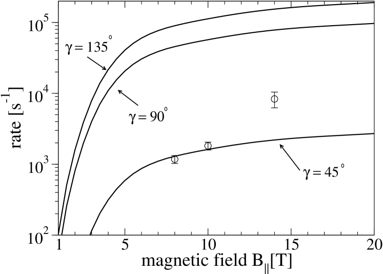
Figure 1: Calculated spin relaxation rate for a single quantum dot as a function of $B_{||}$ applied along $[110]$, $[010]$, and $[\bar{1}10]$. The symbols are experimental data from Ref. Elzerman et al., 2004. The calculated curves for $B_{||}\gtrsim 10$ T are not realistic since they do not incorporate cyclotron effects in the $z$ direction.

While spin-orbit terms couple opposite spin states, electron-phonon coupling enables transitions between such states. Here we include the most relevant terms—deformation and piezoelectric acoustic electron-phonon potentials (direct spin-dependent electron-phonon couplings appear inefficient Khaetskii and Nazarov (2000, 2001)),

$$H_{\rm ep}=\sum_{{\bf Q}\lambda}\sqrt{\frac{\hbar Q}{2\rho Vc_{\lambda}}}\Big{(}\sigma_{e}\delta_{l\lambda}-\frac{ieh_{14}M_{\lambda}}{\sqrt{Q}}\Big{)}(b_{{\bf Q}\lambda}+b^{\dagger}_{-{\bf Q}\lambda})e^{i{\bf q}\cdot{\bf r}}.$$ (5)

The summation is over phonon wave vectors ${\bf Q}=({\bf q},Q_{z})$ and polarizations $\lambda$ (two acoustic, $t$, and one longitudinal, $l$). The phonon creation and annihilation operators are denoted by $b^{\dagger}$ and $b$, respectively. For GaAs the mass density is $\rho=5.3\times 10^{3}$ kg/$m^{3}$, the phonon velocities are $c_{l}=5.3\times 10^{3}$ m/s and $c_{t}=2.5\times 10^{3}$ m/s, the deformation potential $\sigma_{e}=7.0$ eV, and the piezoelectric constant $eh_{14}=1.4\times 10^{9}$ eV/m; $V$ is the unit cell volume and $N$ is the number of unit cells. The geometric factors $M_{\lambda}$ depend only on the direction of ${\bf Q}$ Mahan (2000).

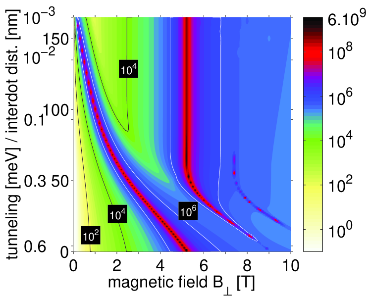
Figure 2: (Color online) Calculated spin relaxation, in s^-1, for a double quantum dot along [100] as a function of a perpendicular magnetic field $B_{\perp}$ and tunneling energy/interdot distance. The labeled contours are equirelaxational lines. Three spin hot spot “ridges” are visible with spin relaxation as large as $10^{9}$ s^-1. The granular pattern at spin hot spots is due to the finite resolution of the graphics.

We calculate the rate of spin relaxation as the transition probability (given by the Fermi golden rule) due to $H_{\rm ep}$, from the upper Zeeman split ground state (denoted as $\Gamma^{\downarrow}_{S}$ in Stano and Fabian (2005)) to all lower states (which have necessarily opposite spin). If the Zeeman splitting is smaller than the orbital excitation energy, the spin relaxes to the ground state ($\Gamma_{S}^{\uparrow}$) only. If, however, more orbital states are present below the upper Zeeman split state, transitions to all lower states contribute to spin relaxation. This is particularly relevant for spin relaxation in single dots at large magnetic fields and in coupled dots at weak couplings. The spin direction of a state is given by the sign of the expectation value of $\boldsymbol{\sigma}$ in the direction of ${\bf B}$.

In order to predict the spin relaxation rate in coupled dots, we first discuss a single dot case and compare it with experiment. This is shown in Fig. 1, where spin relaxation as a function of $B_{||}$ applied at different angles $\gamma$ is calculated. The experiment specific value of $g=-0.35$ is taken. Spin-orbit parameters could be adjusted from a fit to the experimental data. However, such a fit is presently not possible since the calculated rates depend strongly on $\gamma$, reflecting the reduced symmetry ($C_{2v}$) of the GaAs interface, while the experimental data are taken for a single diagonal crystallographic direction, undetermined whether [110] or $[1\overline{1}0]$ with respect to $C_{2v}$) Van . These two directions are not equivalent, which is reflected by the anisotropy shown in Fig. 1. For the purposes of demonstration we assume ad hoc that the experiment is done for [110]; the spin-orbit parameters used in this paper are selected (the selection is by no means unique) to quantitatively describe the experiment with this $\gamma$ foo . This is to demonstrate that the experiment is consistent with the phonon-induced spin relaxation model for reasonable values of spin-orbit parameters. We disagree with the experiment at 14 T in which cyclotron effects (beyond the scope of our theory) in the growth direction become important.

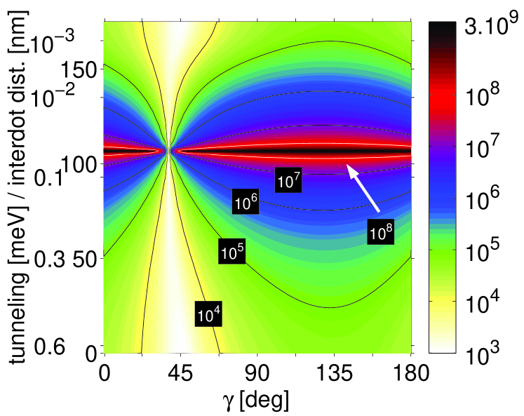
Figure 3: (Color online) Calculated spin relaxation rate, in s^-1, of a double quantum dot as a function of $\gamma$ and tunneling energy, for $B_{||}=5$ T. The dots are oriented along [100]. The weakest relaxation is for $\gamma\approx 35^{\circ}$. Spin hot spots strongly influence spin relaxation at tunneling energies from 0.001 to 0.1 meV.

The calculated anisotropy in Fig. 1 appears due to the reduced symmetry in the presence of both Bychkov-Rashba and Dresselhaus terms Stano and Fabian (2005). Using a unitary transformation that eliminates the linear spin-orbit terms in a confined system Aleiner and Fal’ko (2001); Stano and Fabian (2005) the Zeeman term due to $B_{||}$ transforms to an effective Zeeman term with magnetic field $B^{\rm eff}_{z}(x,y)\hat{z}$ along $z$:

$$B^{\rm eff}_{z}=-B_{||}\left[x\left(\frac{\cos\gamma}{l_{BR}}-\frac{\sin\gamma}{\l_{D}}\right)+y\left(\frac{\sin\gamma}{l_{BR}}-\frac{\cos\gamma}{l_{D}}\right)\right].$$ (6)

The spin-flip probability is proportional to the square of the transition matrix element of $B^{\rm eff}_{z}$. Since the single dot (Fock-Darwin) upper and lower Zeeman ground states are coupled through the first excited orbital states which can be chosen to have a definite $x$ or $y$ symmetry, the spin relaxation rate is proportional to the sum of the squares at $x$ and $y$ in Eq. 6. The spin-flip probability is then proportional to the inverse of the square of the effective anisotropic spin-orbit length ${\cal L}_{SO}(\gamma)$,

$${\cal L}^{-2}_{SO}(\gamma)=1/l_{BR}^{2}+1/\l_{D}^{2}-2\sin(2\gamma)/l_{BR}l_{D}.$$ (7)

The period of $\pi$ reflects the $C_{2v}$ symmetry of the interface Stano and Fabian (2005). The minimum spin relaxation is at $\gamma=45^{\circ}$, while the maximum is at $135^{\circ}$, consistent with the numerics in Fig. 1. The anisotropy is absent if one of the spin-orbit couplings dominates. Experimental observation of such an anisotropy would be a clear signal of a phonon-induced spin relaxation and could be used to extract the ratio of $l_{D}$ and $l_{BR}$. If $l_{BR}=l_{D}$, the anisotropy is strongest—the spin relaxation rate due to the linear spin-orbit terms vanishes for $\gamma=45^{\circ}$. Details of the analytical derivations will be published in a longer version of this article Sta . The anisotropy of Eq. 7 has been found earlier Golovach et al. (2004), while related anisotropies in g-factors has been predicted for extended two-dimensional systems Valin-Rodriguez and Nazmitdinov (2005).

We now move to double quantum dots described by the confining potential $V$ in Eq. 1. We have already predicted that spin hot spots in these systems appear whenever the Zeeman splitting equals the tunneling energy (difference between symmetric and asymmetric orbital levels) Stano and Fabian (2005). At weak coupling ($d\gg l_{0}$) the Zeeman splitting dominates and spin relaxation proceeds through at least two channels, one to the symmetric ($\Gamma_{S}^{\uparrow}$), the other to the asymmetric ($\Gamma_{A}^{\uparrow}$) orbital state. At large coupling spin relaxation is, in general, a single channel process, except at very large magnetic fields in which Landau levels form. The two regimes are separated by a spin hot spot in which spin relaxation is as large as orbital relaxation. This regime is common—typical values for the tunneling energy and the Zeeman splitting are of order 0.1 meV.

Consider first double dots with a perpendicular magnetic field $B_{\perp}$ which contributes both the Zeeman splitting as well as cyclotron effects. The calculated spin relaxation as a function of tunneling energy and $B_{\perp}$ is shown in Fig. 2. The profile is rather complex. Spin relaxation is dominated by the presence of spin hot spots which enhance spin relaxation in most regimes of the control parameters. For tunneling energies below 0.2 meV the weakest spin relaxation is for magnetic fields from 2 to 5 T. At $d=0$ the calculated rate is that of single quantum dots. There is a characteristic cusp structure as a function of $B_{\perp}$ at a spin hot spot at $B_{\perp}\approx 5$ T (such a cusp is not seen for the in-plane field case in Fig.1 since due to the absence of cyclotron effects the spin-hot spots appear at large fields of $B_{||}\approx 54$ T). Our calculation for this single-dot case is in quantitative agreement with perturbative calculationsBulaev and Loss (2005a).

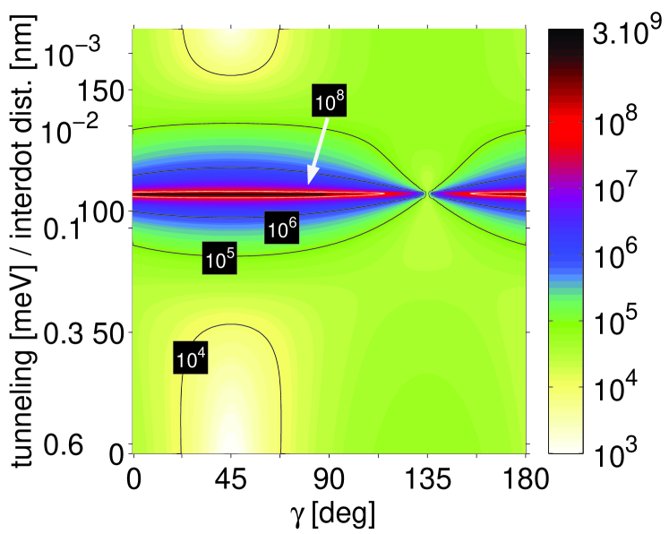
Figure 4: (Color online) Calculated spin relaxation, in s^-1, of a double dot as a function of $\gamma$ and the tunneling energy, for $B_{||}=5$ T. The dots are oriented along [110]. The weakest spin relaxation is for $\gamma=135^{\circ}$, while at $\gamma=45^{\circ}$ spin hot spots do appear.

Let us now look at spin relaxation in an in-plane field $B_{||}$, a situation interesting for spin qubit experiments, since cyclotron effects are inhibited. Two important cases are shown for $B_{||}=5$ T and different orientations $\delta$. The first case, in which the dots are along [100], is shown in Fig. 3, and the second case, in which the dots are along [110], is shown in Fig. 4. At small and large couplings, the spin relaxation rate is strongly anisotropic, similar to the single-dot case in Fig. 1. This anisotropy is greatly enhanced in the intermediate coupling by spin hot spots. In fact, spin hot spots dominate this useful regime: spin relaxation is several orders of magnitude higher than in the single dot case (limits of either very strong or very weak coupling on the graph) at virtually all $\gamma$. The exceptions are $\gamma\approx 35^{\circ}$ in Fig. 3 and $\gamma=135^{\circ}$ in Fig. 4. At smaller (larger) $B_{||}$, the strong relaxation regime moves towards smaller (larger) coupling, while the two angles of “easy passage” remain.

The anisotropy in both $\gamma$ and $\delta$ can be explained by transforming the effective Zeeman field $B^{\rm eff}_{z}$, Eq. 6, into the rotated coordinate system in which the $x$ axis lies along ${\bf d}$:

$$\tilde{B}^{\rm eff}_{z} = -B_{||}x\left[l_{BR}^{-1}\cos(\gamma-\delta)-l_{D}^{-1}\sin(\gamma+\delta)\right]$$ (8)

$$+ B_{||}y\left[l_{BR}^{-1}\sin(\gamma-\delta)-l_{D}^{-1}\cos(\gamma+\delta)\right].$$

Unlike in single dots, the relevant states in double dots are coupled by $x$ and $y$ differently. At weak coupling the dominant term is the one containing $x$ (which is the symmetry of the first excited orbital state $\Gamma_{A}$ Stano and Fabian (2005)). This term leads to anisotropic spin hot spots and giant spin relaxation seen in Figs. 3 and 4. Spin hot spots vanish if $l_{BR}^{-1}\cos(\gamma-\delta)-l_{D}^{-1}\sin(\gamma+\delta)=0$, which, for $\delta=0$, gives $\tan\gamma=l_{D}/l_{BR}$. For our parameters the corresponding angle is about 35^∘, consistent with the numerical calculation shown in Fig. 3. Unfortunately, this angle depends on the spin-orbit coupling and is thus not robust against materials and growth details. On the other hand, for $\delta=45^{\circ}$, the spin hot spots vanish if $\gamma=135^{\circ}$, which is a universal value independent of spin-orbit coupling. This is confirmed numerically in Fig. 4. In the special case of $l_{BR}=l_{D}$, the condition for the weakest spin relaxation would be $\gamma=45^{\circ}$, as in single dots.

In GaAs single dots spin hot spots, which appear at large magnetic fields, are due to the Bychkov-Rashba coupling only Bulaev and Loss (2005a); Stano and Fabian (2005). On the other hand, as can be read from Eq. 8, in double dots spin hot spots appear at arbitrary small magnetic fields and are caused by both the Bychkov-Rashba and Dresselhaus couplings Stano and Fabian (2005), whose interference causes spin hot spot anisotropy.

Similar results apply for other growth directions. In [111] $H_{D}\sim H_{BR}$ Žutić et al. (2004) and the above results in the limit $\l_{D}\to\infty$ apply (with $l_{BR}$ being a combination of both coupling strengths). The spin hot spots are inhibited for any orientation of double dots and a perpendicular in-plane field [$\cos(\gamma-\delta)=0$]; such a configuration can also be used in applications. In the [110] case a unique easy passage exists for $\gamma=0$ and $\delta=90^{\circ}$ Sta .

In conclusion, we have performed realistic calculations of phonon-induced spin relaxation in double quantum dots in the presence of magnetic field. The spin relaxation rate is dominated by spin hot spots in the useful regime of interdot couplings. The spin hot spot anisotropy allows an inhibited spin relaxation for the dots oriented along a diagonal of the [001] plane with a transverse in-plane magnetic field.

We thank U. Rössler for useful discussions. This work was supported by the US ONR.

References

- Loss and DiVincenzo (1998) D. Loss and D. P. DiVincenzo, Phys. Rev. A 57, 120 (1998).
- Fabian and Hohenester (2005) J. Fabian and U. Hohenester, Phys. Rev. B 72, 201304 (2005).
- Khaetskii and Nazarov (2000) A. V. Khaetskii and Y. V. Nazarov, Phys. Rev. B 61, 12639 (2000).
- Khaetskii and Nazarov (2001) A. V. Khaetskii and Y. V. Nazarov, Phys. Rev. B 64, 125316 (2001).
- Woods et al. (2002) L. M. Woods, T. L. Reinecke, and Y. Lyanda-Geller, Phys. Rev. B 66, 161318 (2002).
- Golovach et al. (2004) V. N. Golovach, A. Khaetskii, and D. Loss, Phys. Rev. Lett. 93, 016601 (2004).
- Cheng et al. (2004) J. L. Cheng, M. W. Wu, and C. Lü, Phys. Rev. B 69, 115318 (2004).
- Destefani and Ulloa (2004) C. F. Destefani and S. E. Ulloa (2004), eprint cond-mat/0412520.
- Bulaev and Loss (2005a) D. V. Bulaev and D. Loss, Phys. Rev. B 71, 205324 (2005a).
- Falko et al. (2005) V. I. Falko, B. L. Altshuler, and O. Tsyplyatyev, Phys. Rev. Lett. 95, 076603 (2005).
- Sherman and Lockwood (2005) E. Y. Sherman and D. J. Lockwood, Phys. Rev. B 72, 125340 (2005).
- Calero et al. (2005) C. Calero, E. M. Chudnovsky, and D. A. Garanin, Phys. Rev. Lett. 95, 166603 (2005).
- Bulaev and Loss (2005b) D. V. Bulaev and D. Loss, Phys. Rev. Lett. 95, 076805 (2005b).
- Tsitsishvili et al. (2005) E. Tsitsishvili, R. v. Baltz, and H. Kalt, Phys. Rev. B 72, 155333 (2005).
- Romano et al. (2005) C. L. Romano, P. I. Tamborenea, and S. E. Ulloa (2005), eprint cond-mat/0508303.
- Elzerman et al. (2004) J. M. Elzerman, R. Hanson, L. H. Willems van Beveren, B. Witkamp, L. M. K. Vandersypen, and L. P. Kouwenhoven, Nature 430, 431 (2004).
- Fabian and Das Sarma (1998) J. Fabian and S. Das Sarma, Phys. Rev. Lett. 81, 5624 (1998).
- Fabian and Das Sarma (1999) J. Fabian and S. Das Sarma, Phys. Rev. Lett. 83, 1211 (1999).
- Stano and Fabian (2005) P. Stano and J. Fabian, Phys. Rev. B 72, 155410 (2005).
- Žutić et al. (2004) I. Žutić, J. Fabian, and S. Das Sarma, Rev. Mod. Phys. 76, 323 (2004).
- de Sousa and Das Sarma (2003) R. de Sousa and S. Das Sarma, Phys. Rev. B 67, 033301 (2003).
- Miller et al. (2003) J. B. Miller, D. M. Zumbühl, C. M. Marcus, Y. B. Lyanda-Geller, D. Goldhaber-Gordon, K. Campman, and A. C. Gossard, Phys. Rev. Lett. 90, 076807 (2003).
- Knap et al. (1996) W. Knap, C. Skierbiszewski, A. Zduniak, E. Litwin-Staszewska, D. Bertho, F. Kobbi, J. L. Robert, G. E. Pikus, F. G. Pikus, S. V. Iordanskii, et al., Phys. Rev. B 53, 3912 (1996).
- Mahan (2000) G. D. Mahan, Many-particle Physics (Kluwer, New York, 2000).
- (25) L. M. K. Vandersypen, private communication.
- (26) If we took the direction to correspond to the experimental situation, the spin-orbit parameters would need to have values at the lower limit of what appears to be realistic for GaAs systems.
- Aleiner and Fal’ko (2001) I. L. Aleiner and V. I. Fal’ko, Phys. Rev. Lett. 87, 256801 (2001).
- (28) P. Stano and J. Fabian, unpublished.
- Valin-Rodriguez and Nazmitdinov (2005) M. Valin-Rodriguez and R. G. Nazmitdinov (2005), eprint cond-mat/0512231.