Alternate solitons: Nonlinearly-managed one- and two-dimensional solitons in optical lattices

Abstract

We consider a model of Bose-Einstein condensates which combines a stationary optical lattice (OL) and periodic change of the sign of the scattering length (SL) due to the Feshbach-resonance management. Ordinary solitons and ones of the gap type being possible, respectively, in the model with constant negative and positive SL, an issue of interest is to find solitons alternating, in the case of the low-frequency modulation, between shapes of both types, across the zero-SL point. We find such alternate solitons and identify their stability regions in the 2D and 1D models. Three types of the dynamical regimes are distinguished: stable, unstable, and semi-stable. In the latter case, the soliton sheds off a conspicuous part of its initial norm before relaxing to a stable regime. In the 2D case, the threshold (minimum number of atoms) necessary for the existence of the alternate solitons is essentially higher than its counterparts for the ordinary and gap solitons in the static model. In the 1D model, the alternate solitons are also found only above a certain threshold, while the static 1D models have no threshold. In the 1D case, stable antisymmetric alternate solitons are found too. Additionally, we consider a possibility to apply the variational approximation (VA) to the description of stationary gap solitons, in the case of constant positive SL. It predicts the solitons in the first finite bandgap very accurately, and does it reasonably well in the second gap too. In higher bands, the VA predicts a border between tightly and loosely bound solitons.

I Introduction

Photonic lattices, i.e., effective periodic potentials created by the interference of counter-propagating laser beams in quasi-linear modes, provide for a powerful tool for the study of nonlinear dynamics in other, nonlinear, modes in the same media. A well-known example is a photonic lattice in a photorefractive medium, where the beams launched in the ordinary polarization are nearly linear, while the bias electric field applied to the crystal makes the orthogonal extraordinary polarization strongly nonlinear. This technique has made it possible to predict prediction and create Photorefr various one- and two-dimensional (1D and 2D) lattice solitons, including localized vortices PhotorefrVortex , in the extraordinary polarization, supported by a harmonic photonic lattice in the ordinary one.

Another physically significant example is provided by solitons in Bose-Einstein condensates (BECs), that were predicted in the presence of optical lattices (OLs) created by laser beams illuminating the condensate (while the mean-field dynamics of the BEC wave function is nonlinear due to effects of collisions between atoms, the medium is completely linear for the optical beams). In particular, 2D BBB1 -BBB3 and 3D BBB1 ; BBB2 OLs were shown to stabilize solitons in BECs with attractive interactions between atoms BBB1 -BBB3 (without the lattice, the corresponding soliton solutions exist too, but they are unstable against the spatiotemporal collapse Berge ). Moreover, it has been demonstrated that low-dimensional OLs, i.e., 1D and 2D lattice in the 2D BBB2 ; BBB3 and 3D BBB2 ; BBB3 ; Barcelona  case, respectively, can also stabilize fully localized multi-dimensional solitons, giving them the freedom to move in the unrestricted directions and thus collide BBB3 . A related result is the demonstration of the stability of 2D Bessel and 3D Dumitru solitons in the models with a cylindrical OL, that can be induced by a diffraction-free Bessel beam (see Ref. Bessel and references therein).

If inter-atomic interactions in the BEC are repulsive (which is the most common case Pethik ), solitons cannot exist in the free space, but they can be created and supported, in the form of gap solitons, by the periodic OL potential Konotop ; Ostrovskaya . The 1D gap solitons have been recently observed in the ⁸⁷Rb condensate Oberthaler . Besides the fundamental solitons of the gap type, stable vortical solitons have also been predicted in the 2D self-repulsive BECs trapped in the square OL BBB2 ; Sakaguchi ; Ostrovskaya2 .

Another mechanism which is was theoretically shown to be an effective tool for the stabilization of 2D solitons in BECs (but not of their 3D counterparts) is periodic temporal modulation of the nonlinearity coefficient, which is possible through the ac Feshbach resonance. In this case, external magnetic field alters the scattering length (SL) of the atomic collisions, and the application of the ac field can periodically change the sign of the interaction. This mechanism is the basis of the so-called Feshbach-resonance-management (FRM) technique FRM (which may be regarded as an implementation of a general concept of the nonlinearity management). A possibility to employ the FRM for the stabilization of 2D solitons – in principle, without any trapping field – has been recently demonstrated Fatkhulla ; Japan ; VPG (in fact, this mechanism follows the pattern of the one proposed earlier for the stabilization of cylindrical optical solitons in a layered medium with the periodically alternating sign of the Kerr coefficient Isaac ). It is also relevant to mention that, while the 1D OL, unlike its 2D and 3D counterparts, cannot stabilize 3D solitons BBB3 , and the FRM technique per se does not make it possible either, a combination of the FRM and one-dimensional OL readily stabilizes single- and multi-peaked solitons in the 3D space Michal .

Thus, two distinct kinds of solitons are possible in BECs, under stationary conditions: ordinary ones in the case of self-attraction, and gap solitons in the case of repulsion. The OL is necessary for the existence of the gap solitons in any dimension, and for the stability of the ordinary ones, except for the 1D case, where ordinary solitons are stable without the lattice (only in this case ordinary solitons have been already observed in the experiment experiment ). Solitons of the two kinds differ not only by their existence and stability conditions, but also in the shape: ordinary solitons normally have a single-peak structure without zeros, while the gap solitons feature oscillatory tails with many zero-crossings.

The possibility of the application of the above-mentioned FRM technique suggests to consider a “mixed” situation, when the sign of the nonlinearity periodically changes between the attraction and repulsion. In the case of the high-frequency “management”, the application of the averaging method makes this situation tantamount to that in an effective static model Fatkhulla . However, in the quasi-adiabatic (low-frequency) case, one may expect time-periodic alternation between solitons of the two types. Such alternate solitons, which were not considered before, is the subject of the present work. In particular, an issue is whether they are able to survive periodic passage of the zero-SL point, as no soliton can exist in the static model without nonlinearity. In this work, we chiefly focus on the 2D case, which is the most interesting one; however, the 1D model is considered too – in particular, with the objective to compare conclusions concerning the stability of alternate solitons in the different dimensions, and the necessary conditions (threshold) for their existence.

Besides that, we also consider a more specific issue that was not studied before, viz., a possibility to apply the well-known technique of the variational approximation (VA) Progress to stationary gap solitons in OLs. Nevertheless, the main results reported in this work are based on direct numerical simulations, as the VA technique for the alternate solitons in the time-modulated system is too cumbersome.

The paper is organized as follows. In Section 2, we formulate the model, including the consideration of its linear spectrum, and present results generated by the VA for static 2D gap solitons on the square lattice. The most essential results for the 2D alternate solitons are reported in Section 3, and respective results for the 1D model are given in Section 4. The paper is concluded by Section 5. Some technical details of the VA are presented in the Appendix.

II The model, linear spectrum, and variational approximation

In the mean-field approximation, the evolution of the BEC single-atom wave function $\psi$ in the presence of the 2D square-shaped OL and a tight trap in the transverse (third) direction obeys an effective two-dimensional Gross-Pitaevskii equation. Its normalized form is well known Pethik :

$$i\frac{\partial\psi}{\partial t}+\frac{\partial^{2}\psi}{\partial x^{2}}+\frac{\partial^{2}\psi}{\partial y^{2}}+\varepsilon\left[\cos(2x)+\cos(2y)\right]\psi+\lambda(t)|\psi|^{2}\psi=0,$$ (1)

where $\varepsilon$ is the strength of the square lattice, its spatial period scaled to be $\pi$. In this work, we focus on solitons which may exist in a large-area domain without the support from an external parabolic-potential trap, therefore Eq. (1) does not include the latter term. The nonlinear coefficient $\lambda(t)$ in Eq. (1) is proportional to the SL of atomic collisions, which is controlled by the ac magnetic field through the Feshbach resonance. The positive and negative signs of $\lambda$ correspond to the self-attractive and repulsive condensate, respectively. The only dynamical invariant of Eq. (1) (with the time-dependent $\lambda(t)$) is the norm, which is proportional to the number of atoms in the condensate,

$$N=\int\int\left|\psi(x,y,t)\right|^{2}dxdy.$$ (2)

In case of $\lambda=\mathrm{const}$, stationary solutions are sought as $\psi(x,y,t)=u(x,y)\exp(-i\mu t)$ with a real chemical potential $\mu$ and a real function $u$ satisfying the equation

$$\mu u+\frac{\partial^{2}u}{\partial x^{2}}+\frac{\partial^{2}u}{\partial y^{2}}+\varepsilon\left[\cos(2x)+\cos(2y)\right]u+\lambda u^{3}=0$$ (3)

The search for soliton solutions should be preceded by consideration of the spectrum of the linearized version of Eq. (3), as solitons may only exist at values of $\mu$ belonging to gaps in the spectrum. The linearization of Eq. (3) leads to a separable 2D eigenvalue problem,

$$\left(\hat{L}_{x}+\hat{L}_{y}\right)u(x,y)=-\mu u(x,y),$$ (4)

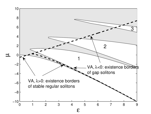
Figure 2: The band-gap structure and regions of the existence of regular ($\lambda>0$) and gap ($\lambda<0$) solitons, as predicted by the variational approximation based on the Gaussian ansatz. Shaded and unshaded zones are, respectively, the Bloch bands (where solitons cannot exist) and gaps (where solitons are possible). Dashed lines are borders of the soliton existence regions.

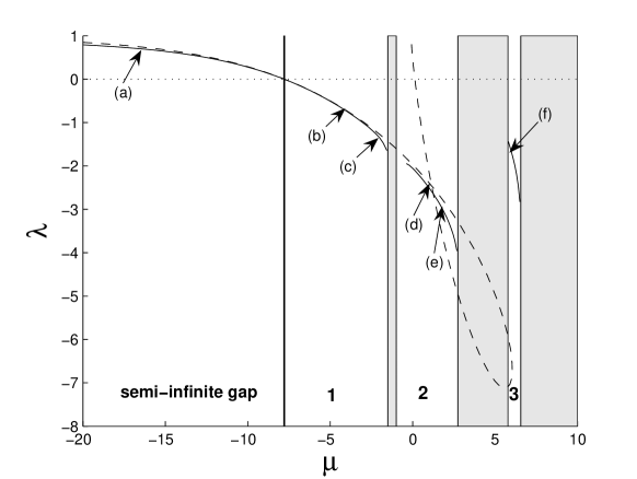
Figure 3: Comparison of the numerically generated soliton family and the one predicted by the variational approximation (solid and dashed lines, respectively) for the fixed value of the optical-lattice’s strength, $\varepsilon=7.5$. Shaded and unshaded zones are the Bloch spectral bands and gaps, respectively.

where we have defined the 1D linear operator $\hat{L}_{x}\equiv\partial^{2}/\partial x^{2}+\varepsilon\cos(2x)$. The corresponding eigenstates can be built as $u_{kl}(x,y)=g_{k}(x)g_{l}(y)$, with the eigenvalues $\mu_{kl}=\mu_{k}+\mu_{l}$, where $g_{k}(x)$ and $g_{l}(y)$ is any pair of quasi-periodic Bloch functions solving the Mathieu equation, $\hat{L}_{x}g_{k}(x)=-\mu_{k}g_{k}(x)$, $\mu_{k}$ and $\mu_{l}$ being the corresponding eigenvalues. The band structure of the 2D linear equation (4) constructed this way was already investigated in detail (see, e.g., Refs. Ostrovskaya and DemetriMoti ). It includes, as usual, a semi-infinite gap which extends to $\mu\rightarrow-\infty$, and a set of finite gaps separated by bands that are populated by quasiperiodic Bloch-wave solutions, see Figs. 2 and 3 below.

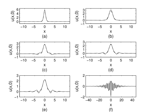
Figure 4: Comparison of the soliton profiles found numerically and those generated by the variational approximation (solid and dashed lines, respectively) for the same fixed value of the optical-lattice’s strength as in Fig. 3, $\varepsilon=7.5$. Plots (a) to (f) correspond to points in the parameter plane ($\mu$, $\lambda$) labeled by the same symbols in Fig. 3. This figure and Fig. 5 show cross sections of the two-dimensional solitons along the axis $y=0$.

With the self-attractive nonlinearity ($\lambda>0$), a family of stable stationary 2D solitons was found in the semi-infinite gap BBB1 ; Yang ; DemetriMoti . With the repulsive nonlinearity, $\lambda<0$, stable 2D gap-soliton solutions can be found in finite gaps Konotop ; Ostrovskaya ; BBB2 ; Sakaguchi . In either case, a necessary condition for the existence of the stationary 2D solitons is that their norm (see Eq. (2)) exceeds a certain minimum (threshold) value, $N_{\mathrm{thr}}$ DemetriMoti (see some details below). Further, both the ordinary and gap-mode solitons generated by Eq. (3) with $\lambda>0$ and $\lambda<0$, respectively, can be categorized (following Ref. Sakaguchi ) as tightly-bound (TB) and loosely-bound (LB) ones. TB solitons are essentially confined to a single cell of the OL potential, with weak tails extending into adjacent cells (for this reason, similar solutions were called single-cell solitons in Ref. BBB1 ). On the contrary, LB solitons (alias multi-cell ones BBB1 ) extend over many lattice cells; examples of both types of the soliton’s shape are given below in Fig. 4.

The TB solitons are well approximated by a Gaussian ansatz, which is a basis for the application of the variational approximation (VA) to them, as it was done in Refs. BBB1 ; BBB2 ; BBB3 for the self-attraction case (the VA was first applied to BEC models in Refs. VA ). The Lagrangian corresponding to the stationary equation (3) is

$$L=\int_{-\infty}^{+\infty}\left\{\mu u^{2}-\left[\left(\frac{\partial u}{\partial x}\right)^{2}+\left(\frac{\partial u}{\partial y}\right)^{2}\right]+\frac{1}{2}\lambda u^{4}+\varepsilon\left[\cos(2x)+\cos(2y)\right]u^{2}\right\}dx.$$ (5)

The Gaussian ansatz is taken in the form of

$$u(x,y)=A\exp\left(-\frac{x^{2}+y^{2}}{2a^{2}}\right),$$ (6)

which assumes that the soliton’s center is pinned at a local potential minimum, $x=y=0$ (it is a minimum provided that we set $\varepsilon>0$). Substitution of the ansatz in the expression (5) yields the effective Lagrangian,

$$L_{\mathrm{eff}}=\pi A^{2}\left[\mu a^{2}-1+\frac{\lambda}{4}A^{2}a^{2}+2\varepsilon a^{2}\exp\left(-a^{2}\right)\right].$$ (7)

This effective Lagrangian was already found in Ref. BBB1 and used, as said above, to predict TB solitons in the case of the attractive nonlinearity, with $\lambda=+1$ . Here, we do not fix $\lambda$; instead, we fix the solution’s norm (2),

$$N_{\mathrm{sol}}=\pi A^{2}a^{2}\equiv 4\pi.$$ (8)

The variational equations following from the Lagrangian (7), $\partial L_{\mathrm{eff}}/\partial\left(A^{2}\right)=\partial L_{\mathrm{eff}}/\partial\left(a^{2}\right)=0$, along with the normalization condition (8), lead to relations $A=2/a$ and

$$\lambda = 1-2\varepsilon a^{4}\exp\left(-a^{2}\right),~{}$$ (9)

$$\mu = -a^{-2}-2\varepsilon\left(1-2a^{2}\right)\exp\left(-a^{2}\right),$$ (10)

Equation (9) with $\varepsilon>0$ generates two physical solutions (ones with $a^{2}>0$) in the interval

$$1-8e^{-2}\varepsilon\leq\lambda\leq 1$$ (11)

BBB1 (in the case of $\varepsilon=0$, the interval shrinks to the single point $\lambda=1$, which precisely corresponds to the (unstable) Townes soliton of the free-space 2D nonlinear Schrödinger equation Berge ).

In the case of self-attraction, $\lambda>0$, the existence interval (11) is present for any $\varepsilon$ BBB1 , and, for a relatively weak OL, with $\varepsilon<\varepsilon_{\mathrm{cr}}=e^{2}/8\approx 0.92$, Eq. (11) predicts a threshold condition for the existence of the 2D soliton, $\lambda>\lambda_{\mathrm{thr}}\equiv 1-8e^{-2}\varepsilon$. The latter implies the existence of the above-mentioned threshold value of the norm, if $N$ is allowed to vary while $\lambda$ is fixed. For a strong lattice, with $\varepsilon>\varepsilon_{\mathrm{cr}}$, Eq. (11) formally predicts zero threshold; however, as was shown in Ref. BBB1 , the latter prediction is an artifact of the VA. In reality, a finite $\lambda_{\mathrm{thr}}$ for fixed $N$, or, equivalently, finite $N_{\mathrm{thr}}$ for fixed $\lambda$ is always present. A delocalization transition which happens beneath the threshold was investigated in detail (including the three-dimensional case) in Ref. Salerno . Moreover, a threshold necessary for the formation of solitons was also found in the discrete version of the 2D model Kim . Actually, the threshold is found in the 2D model with any nonlinearity which can support solitons, in combination with the lattice potential DemetriMoti (including 2D models with a quasi-1D potential BBB2 ; BBB3 ), while in the 1D models the threshold is absent.

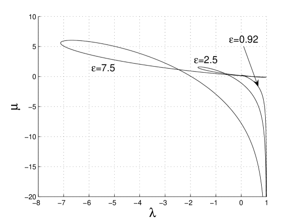
Figure 1: The chemical potential $\mu$ vs. the nonlinearity coefficient $\lambda$ for the soliton family, as given by the variational approximation for different values of the optical-lattice strength $\varepsilon$.

For $\varepsilon>\varepsilon_{\mathrm{cr}}\equiv e^{2}/8$, Eq. (11) predicts too that the solitons may exist in the case of the repulsive nonlinearity, $\lambda<0$, as the expression on the left-hand-side of Eq. (11), $1-\varepsilon/\varepsilon_{\mathrm{cr}}$, is negative in this case. Unlike the above-mentioned formally predicted zero threshold for $\varepsilon>\varepsilon_{\mathrm{cr}}$ and $\lambda>0$, this effect is a real one, as confirmed by numerical results displayed below (in Figs. 3 and 4). Figure 1 shows the chemical potential $\mu$ versus the nonlinearity coefficient $\lambda$, as found from Eqs. (9) and (10). As is seen, the solution curve indeed extends to negative $\lambda\$for $\varepsilon>\varepsilon_{\mathrm{thr}}$, forming a loop.

The existence region for the 2D solitons, as predicted by the VA, is shown in Fig. 2, against the backdrop of the band structure of the 2D model. According to what was said above, two existence borders of the gap solitons, both pertaining to the self-repulsion, $\lambda<0$, meet and terminate, forming a cusp, at the above-mentioned value, $\varepsilon=\varepsilon_{\mathrm{thr}}\approx 0.92$. The lower border very accurately follows a narrow Bloch band separating the first finite gap from the semi-infinite one, in which the ordinary solitons (corresponding to the self-attraction, $\lambda>0$) are predicted to exist. On the other hand, the upper existence border predicted by the VA for the gap solitons cannot be accurate since, in higher finite gaps, the actual soliton’s shape (see examples in Fig. 4 below) is very far from the Gaussian ansatz adopted above. However, comparison with numerically found shapes of the solitons demonstrates that this upper border gives, as a matter of fact, quite an accurate approximation for a separatrix between regions of tightly and loosely bound (TB and LB) solitons in the repulsion case.

Fixing the OL’s strength at $\varepsilon=7.5$, we solved the stationary equation (3) numerically and compared the results with the VA prediction, as shown in Figs. 3 and 4. We observe that, in the semi-infinite and first finite gaps, the accuracy of the prediction for both $\lambda>0$ and $\lambda<0$ (attraction and repulsion) is very good, and in the second finite gap it is fair. The third finite gap is located just above the VA-predicted upper border of the existence region for the gap solitons (the upper dashed line in Fig. 2). The solitons found numerically in the third gap, see panel (f) in Fig. 4, are definitely of the LB type, and they cannot be approximated by the Gaussian ansatz.

We tried to apply the VA to loosely bound (LB) solitons, introducing an ansatz that allows oscillatory tails, cf. Fig. 4(f):

$$u(x,y)=\left[A+B\left(\cos x+\cos y\right)\right]\exp\left(-\frac{x^{2}+y^{2}}{2a^{2}}\right).$$ (12)

Cumbersome variational equations generated by the substitution of this ansatz in the Lagrangian (5) are given in the Appendix. In Fig. 5 we compare the LB-solitons’ shapes, as predicted by the extended ansatz and found from the direct numerical solution of Eq. (3). As is seen in panel (a), the new ansatz fails to adequately describe sidelobes of a soliton which is intermediate between the TB and LB types. For the LB soliton proper, panel (b) shows that three central peaks are correctly approximated by the modified VA, but the discrepancy is large farther from the center.

III Dynamics of two-dimensional solitons under the Feshbach-resonance management

In this section we address the main issue of the work, viz., solitons driven by the FRM. The consideration is based on direct simulations of Eq. (1) with the norm fixed as per Eq. (8) and the time-dependent nonlinear coefficient,

$$\lambda(t)=\lambda_{0}+\lambda_{1}\cos(\omega t).$$ (13)

We begin with the case of the vanishing dc part, $\lambda_{0}=0$. At $t=0$, we use the initial profile corresponding to a numerically found soliton solution of the stationary equation (3) with $\lambda=\lambda_{1}$ (we set $\lambda_{1}>0$). Systematic simulations demonstrate that it is possible to achieve stable periodic adiabatic alternations between two quasi-stationary soliton shapes, one corresponding to an ordinary soliton belonging to the semi-infinite gap in the case of the attractive nonlinearity, and the other being a gap soliton in one of the finite gaps, which exists with the repulsive nonlinearity. Relaxation of this alternate soliton to a stable regime is accompanied by very weak radiation loss. In the simulations of the 2D case, we incorporated absorbers near boundaries of the integration domain, in order to emulate an infinite space.

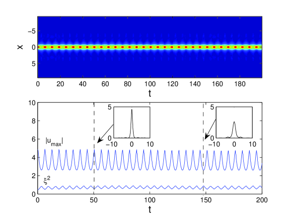
Figure 6: An example of an almost completely stable alternate soliton, for $\varepsilon=5$, $\lambda_{1}=0.7$, $\omega=1$, and $\lambda_{0}=0$; it corresponds to point (a) in Fig. 7 (for $\lambda_{1}=0.7$). The upper panel shows the soliton evolution in terms of contour plots. The lower panel shows the time dependence of the amplitude and mean squared width of the soliton. Two insets are cross-sections of instantaneous profiles of the soliton taken at moments of time ($t=50$ and $t=150$, respectively) when it is very close, respectively, to a regular soliton and one of the gap type.

An example of a robust alternate soliton is given in Fig. 6. In particular, sidelobes in the soliton’s profile, characteristic of the gap-soliton shape, periodically appear and disappear. It is noteworthy that periodic crossings of the zero-SL point, $\lambda=0$, at which no stationary soliton may exist, do not destroy the alternate soliton. The spatially-averaged squared width of the soliton, the temporal evolution of which is shown in the lower panel of the figure, is defined as

$$\xi^{2}(t)\equiv\frac{\int\int x^{2}|u(x,y,t)|^{2}dxdy}{\int\int|u(x,y)|^{2}dxdy}.$$ (14)

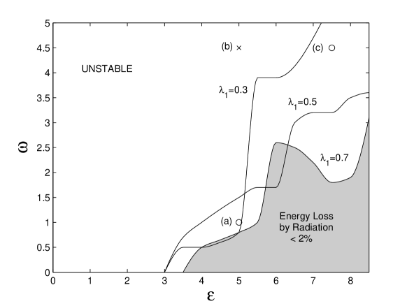
Figure 7: The stability diagram of the alternate solitons in the ($\varepsilon$,$\omega$) plane for $\lambda_{0}=0$ and different fixed values of the Feshbach-resonance-management amplitude $\lambda_{1}$. The region of complete stability (it is shaded for $\lambda_{1}=0.7$) is defined so that the total radiation loss of the soliton’s initial norm is less than $2\%$ in this region.

Results of systematic simulations are summarized in stability diagrams for the alternate solitons, which are displayed in Fig. 7 for $\lambda_{0}=0$ and several different values of the FRM amplitude $\lambda_{1}$. Naturally, the solitons may be stable in the case of the quasi-adiabatic FRM driving, i.e., at sufficiently low frequencies. In the stability region, the total radiation loss is less than $2\%$ of the initial norm (number of atoms), which is our definition of complete robustness of the alternate solitons. In particular, the example shown in Fig. 6 corresponds to the point (a) in Fig. 7 (for $\lambda_{1}=0.7$); in this case, the total loss is almost exactly $2\%$.

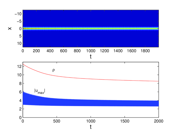
Figure 8: An example of a “semi-stable” soliton, for $\varepsilon=7.5$, $\lambda_{1}=0.7$, $\omega=4.5$, and $\lambda_{0}=0$, which corresponds to point (c) in Fig. 7 (for $\lambda_{1}=0.7$). After 1400 oscillation periods, the soliton definitely survives.

As the driving frequency $\omega$ increases, the soliton emits more radiation. For moderately high frequencies, the initial solitary-wave pulse prepared as said above (i.e., as a numerically exact stationary soliton corresponding to the initial value of $\lambda$) sheds off a conspicuous share of its norm; then, the emission of radiation ceases, and the remaining part of the pulse self-traps into a robust alternate soliton. An example of a such a semi-stable dynamical regime is displayed in Fig. 8. To additionally illustrate the relaxation to the stable regime, the lower panel of the figure includes a plot showing the evolution of the norm,

$$\rho(t)=\int\int|u(x,y,t)|^{2}dxdy,$$ (15)

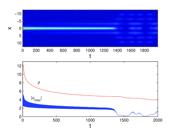
Figure 9: An example of an unstable soliton, for $\varepsilon=5$, $\lambda=0.7$, $\omega=4.5$, and $\lambda_{0}=0$, which corresponds to point (b) in Fig. 7 (for $\lambda_{1}=0.7$). The radiative energy loss almost ceases, but then the soliton gets finally destroyed after about 1000 oscillation periods.

cf. Eq. (14). In this case, the resulting alternate soliton oscillates between near-stationary shapes corresponding to points (a) and (b) in Fig. 3, which belong to the semi-infinite and first finite gaps, respectively. In general, the stronger the OL is, the more robust the alternate soliton will be. In Fig. 7, the semi-stable regimes are not marked separately from completely unstable ones, as the border between them is fuzzy (in particular, it is not quite clear whether the semi-stable solitons would not very slowly decay on an extremely long time scale, unavailable to simulations that we could run). In any case, a broad area adjacent to the one marked as completely stable one in Fig. 7 is actually a region of semi-stability. At still higher driving frequencies, the soliton is definitely destroyed, see a typical example in Fig. 9.

It is not quite clear either if the stability region of the alternate solitons is limited on the side of very small frequencies. Indeed, one may expect that, in the latter case, the soliton spending long time around the zero-SL point, $\lambda=0$, must spread out, and may thus decay; on the other hand, if the soliton is very broad by itself, it may survive this temporary spreading out. The lowest frequency checked in our simulations was $\omega=0.1$, the solitons being unequivocally stable at this value of $\omega$. Still lower frequencies require impractically long simulation times (and extremely large simulation domains). Accumulation of numerical error could impede to draw certain conclusions in this case. Extremely long evolution and very large domains are not relevant either from the viewpoint of experiments with BECs.

It is also relevant to address the issue of the existence of the threshold necessary for the formation of the soliton, which, as explained above, exists for both $\lambda>0$ and $\lambda<0$ in the static 2D models. In the nonstationary (FRM-driven) model with the fixed norm (see Eq. (8)), the threshold manifests itself in the fact that persistent alternate solitons cannot be found if the nonlinearity coefficient is too small, $\lambda_{1}<\left(\lambda_{1}\right)_{\mathrm{thr}}$. Identifying the threshold directly from simulations of Eq. (1) is difficult (as well as locating other precise borders of the existence and stability regions for the alternate solitons, see above). For instance, for the strong lattice with $\varepsilon=7.5$ (cf. the situation for the same value of $\varepsilon$ in the stationary model, as illustrated by Fig. 3), the threshold exists but is so small that its accurate value cannot be identified. This is possible for smaller $\varepsilon$. In particular, for $\varepsilon=4$ we have found $\left(\lambda_{1}\right)_{\mathrm{thr}}\approx 0.15$, which should be compared to the the thresholds found, with the same $\varepsilon=4$ and the same fixed norm (8), for the ordinary and gap solitons in the corresponding static 2D models: $\lambda_{\mathrm{thr}}^{\mathrm{(ord)}}\approx 0.04$, and $\lambda_{\mathrm{thr}}^{\mathrm{(gap)}}\approx-0.04$, respectively. Quite naturally, the dynamical threshold is much higher than its static counterparts; at $\lambda_{1}<\left(\lambda_{1}\right)_{\mathrm{thr}}$, the alternate soliton clearly demonstrates a delocalization transition.

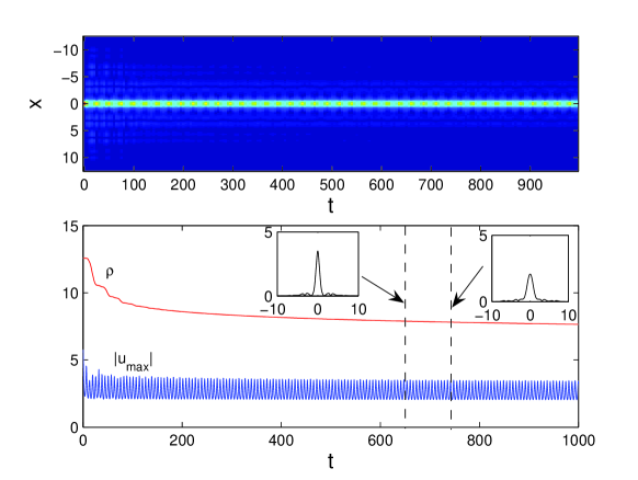
Figure 10: A stable alternate soliton for $\epsilon=7.5$, $\lambda_{0}=-0.9$, $\lambda_{1}=1.6$, and $\omega=1$. The soliton survives while the nonlinear coefficient periodically traverses both the $\lambda=0$ point and two Bloch bands between the semi-infinite and first two finite bands. Insets show cross-sections of instantaneous soliton’s profiles with the largest (left) and smallest (right) amplitudes.

Next, we consider the FRM-driven soliton dynamics with a negative nonzero dc part in Eq. (13), $\lambda_{0}<0$, which corresponds to repulsion. To this end, we consider an example with $\lambda_{0}=-0.9$ and $\lambda_{1}=1.6$. The interaction being repulsive on the average, one may expect the existence of gap solitons in the high-frequency limit. In the simulations, we started with the initial profile corresponding to point (a) in Fig. 3, as the initial value of the nonlinearity coefficient, $\lambda(0)=0.7$, pertains to this point. The minimum instantaneous value of the oscillating nonlinear coefficient is $\lambda_{\min}=-2.5$ in the present case, the stationary solution with $\lambda=-2.5$ pertaining to point (d) in Fig. 3, which belongs to the second finite band. In this regime, the oscillating nonlinear coefficient $\lambda(t)$, in addition to cycling across the point $\lambda=0$ and a very narrow Bloch band separating the semi-infinite and first finite gaps, periodically passes the wider Bloch band between the first and the second finite gaps, where stationary solitons cannot exist. Nevertheless, a stable alternate soliton, found in this case, survives all the traverses of the “dangerous zones”, as shown in Fig. 10. A small amount of radiation is emitted at an initial stage of the evolution, and then a robust alternate soliton establishes itself, cf. Fig. 8. It is noteworthy that, as seen in the insets, this soliton develops sidelobes that actually do not oscillate together with its core, and do not disappear either as $\lambda$ takes positive values. The latter feature distinguishes this stable regime from the one shown in Fig. 6, where the sidelobes periodically disappear.

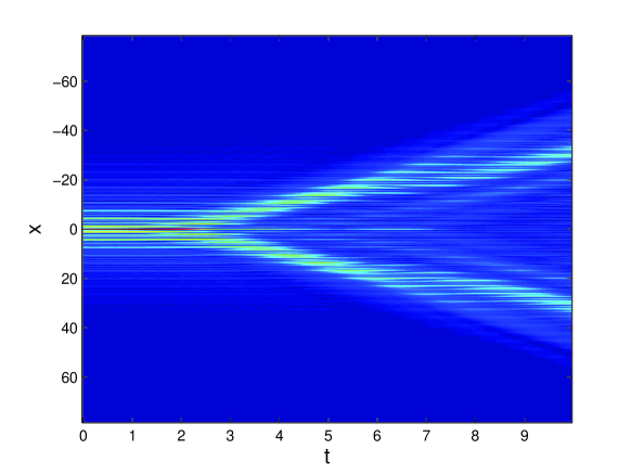
Figure 11: Instability of a loosely bound soliton (with the initial shape similar to that shown in Fig. 4(f)), for $\varepsilon=7.5$, $\lambda_{1}=-1.7$, $\omega=1$, and $\lambda_{0}=0$.

We have also tried to apply the FRM mechanism to weakly localized LB solitons, such as the one in panel (f) of Fig. 4. However, no stable regime periodically passing through a shape of this type could be found for any combination of $\lambda_{0}$ and $\lambda_{1}$ in Eq. (13). A typical example of unstable evolution of FRM-driven LB solitons is displayed in Fig. 11.

IV Dynamics of one-dimensional solitons under the Feshbach-resonance management

The 1D case also deserves consideration, as the experiment may be easier in this case, and it is interesting to compare the results with those reported above for the 2D model. In particular, an issue is whether the existence of the 1D alternate soliton entails any threshold condition. It is well known that the effective 1D Gross-Pitaevskii equation is a straightforward reduction of Eq. (1),

$$i\frac{\partial\psi}{\partial t}+\frac{\partial^{2}\psi}{\partial x^{2}}+\varepsilon\cos(2x)\psi+\lambda(t)|\psi|^{2}\psi=0,$$ (16)

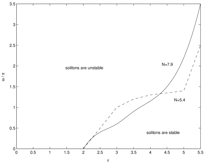
Figure 15: The stability diagram for one-dimensional alternate solitons (cf. the diagram for two-dimensional solitons in 7 ), for $\lambda_{1}=1$ and $\lambda_{0}=0$. The stability borders are shown for two different values of the fixed norm (normalized number of atoms) $N$, to illustrate the generality of the results.

which implies that a tight trap acts in the directions $y$ and $z$. Here we report results only for the (most fundamental) case without the dc component in $\lambda(t)$, i.e., $\lambda_{0}=0$, and fixing $\left|\lambda_{1}\right|=1$ in Eq. (13). The strategy is the same as in the 2D case: direct simulations of Eq. (16) start with a soliton profile that would be a numerically exact stationary soliton for the initial value of the nonlinearity coefficient, $\lambda=\lambda(0)$. In most cases, the solution’s 1D norm was fixed at $N\equiv\int_{-\infty}^{+\infty}\left|u(x)\right|^{2}dx=7.9$ (this normalization was chosen as it corresponds to an almost constant value of the chemical potential, $\mu\approx 2$, in the stationary version of the problem). However, the overall stability diagram will include different values of $N$, see Fig. 15 below.

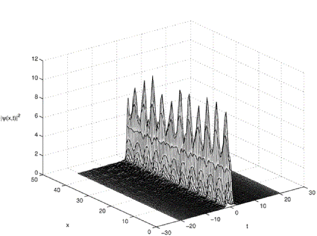
Figure 12: A typical example of a stable alternate soliton found in the one-dimensional model (16), for $\varepsilon=4.5$, $\lambda_{1}=1$, $\omega=\pi/2$, and $\lambda_{0}=0$.

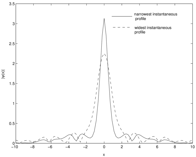
Figure 13: Two profiles between which the stable alternate soliton from the previous figure periodically oscillates.

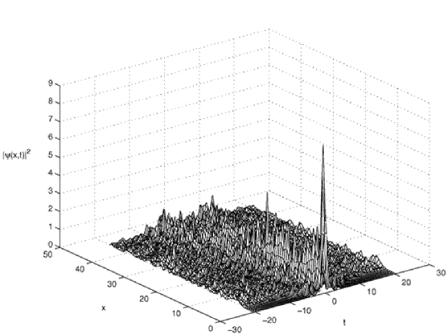
Figure 14: A typical example of the instability of a one-dimensional soliton, for $\varepsilon=3.5$, $\lambda_{1}=1$, $\omega=5\pi/2$, and $\lambda_{0}=0$.

In the 1D case, stable alternate solitons can be readily found, see an example in Fig. 12. The soliton periodically oscillates between the narrow and wide profiles, which are displayed in Fig. 13. Taking a smaller OL’s strength $\varepsilon$ and/or larger frequency $\omega$, we observe onset of strong instability of the soliton, as shown in Fig. 14.

Collecting results of the systematic simulations, we have generated a stability diagram for the 1D alternate solitons, which is displayed in Fig. 15. It is noteworthy that the shape of the stability area is qualitatively similar to that for the 2D case, cf. Fig. 7. The similarity suggest that the basic results for the stability of the alternate solitons are quite generic.

As is well known, in the static 1D models with both $\lambda>0$ and $\lambda<0$, the existence of the ordinary and gap solitons does not require any finite threshold (minimum norm). A principal difference of the dynamic (FRM-driven) 1D model is that persistent alternate solitons can be found only above a finite threshold, $N>N_{\mathrm{thr}}$. Accurate identification of $N_{\mathrm{thr}}$ is rather difficult but possible. For instance, we have found $N_{\mathrm{thr}}\approx 2.1$ for $\varepsilon=7.5$ and $\omega=\pi/2$. Thus, in this sense the 1D dynamic model is closer to the 2D one than to its static 1D counterparts. It remains to investigate the existence of the finite threshold in the 1D dynamic model with a nonzero dc component, i.e., $\lambda_{0}\neq 0$ in Eq. (13).

Besides the fundamental (single-peaked) 1D solitons considered above, stable higher-order (multi-peaked) alternate solitons have been found too. As concerns static higher-order solitons on lattices, a known example is the so-called intrinsic localized mode, i.e., an odd (antisymmetric) soliton in the discrete nonlinear Schrödinger equation ILM . A similar object is a bound state of two lattice solitons, which, too, is stable only in the anti-symmetric configuration, in the 1D Todd and 2D Bishop cases alike.

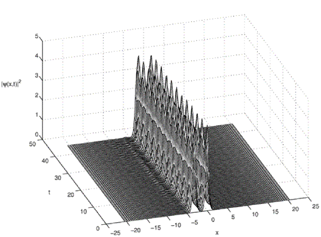
Figure 16: An example of a stable odd (antisymmetric) one-dimensional alternate soliton, for $\lambda_{1}=-1$, $\varepsilon=5$, $\omega=\pi/2$, and $\lambda_{0}=0$.

Following the pattern of the static lattice models, we prepared an antisymmetric initial state as a superposition of two separated solitons (stationary ones corresponding to the initial value of $\lambda$) with opposite signs, i.e., the phase difference of $\pi$. Direct simulations demonstrate that stable alternate antisymmetric solitons can be easily found this way, see a typical example in Fig. 16. Stable solitons of still higher orders, i.e., bound states of several fundamental solitons with the phase shift $\pi$ between them, were found too.

A 2D counterpart of the odd soliton would be a vortical soliton. Such stable vortices were found indeed in the static models with self-attraction BBB1 ; Yang and self-repulsion BBB2 ; Sakaguchi ; Ostrovskaya2 . However, our simulations have not produced stable solitons with intrinsic vorticity in the 2D FRM lattice model based on Eqs. (1) and (13), with $\lambda_{0}=0$.

V Conclusion

We have introduced a model of Bose-Einstein condensates in a system combining the optical lattice (OL) with the strength $\varepsilon~{}$and periodic modulation of the scattering length (SL) with the frequency $\omega$, which is provided by external ac magnetic field through the Feshbach resonance. As it was known before that stationary ordinary solitons and ones of the gap type are possible in the model with constant negative and positive SL, respectively, an issue of interest is to find a stable soliton periodically alternating, in the case of the low-frequency modulation, between shapes of both types. In both 2D and 1D cases, we have found such alternate solitons, and identified their stability regions in the $\left(\varepsilon,\omega\right)$ plane. As might be expected, the stability regions are limited to relatively low frequencies and sufficiently strong OL. A threshold necessary for the formation of the alternate solitons can be found in the 2D model, and also in its 1D counterpart (with the zero mean value of the SL); the latter result is especially interesting, as the 1D static models have no threshold. Dynamical regimes of three types were identified: stable, unstable, and semi-stable, the latter one implying that the initial soliton sheds off a conspicuous part of its norm before relaxing into a stable regime. In the 1D case, stable antisymmetric alternate solitons were additionally found, while stable vortical solitons were not generated by simulations of the 2D model with the zero average SL.

We have also considered a possibility to apply the variational approximation (VA) to the description of stationary gap solitons in the 2D model with a constant positive SL (self-repulsion). We have concluded that the Gaussian ansatz very accurately predicts the solitons in the first finite bandgap, and predicts them with a fair accuracy in the second gap. In higher gaps, the VA actually produces a border between tightly and loosely bound solitons. We also tried to apply a more sophisticated version of the VA, based on the ansatz combining the Gaussian and cosines, with the objective to describe the shape of loosely bound 2D gap solitons with oscillatory tails. It was found that the modified ansatz can correctly describe three central peaks in the soliton’s shape.

Appendix: The variational approximation with the extended ansatz

The effective Lagrangian generated by the substitution of the modified ansatz (12) in Eq. (5) is

$$L_{\mathrm{eff}}=\frac{\pi a^{2}}{16}e^{-4a^{2}}\left\{8B^{3}Ae^{23a^{2}/8}{\left(1+3e^{a^{2}/2}\right)}^{2}\lambda+B^{4}e^{2a^{2}}{\left(1+e^{a^{2}/4}\right)}^{4}{\left(1-2e^{a^{2}/4}+3e^{a^{2}/2}\right)}^{2}\lambda+\right.\\ 32BAe^{7a^{2}/4}\left[{\left(1+e^{a^{2}}\right)}^{2}\varepsilon+e^{2a^{2}}\left(A^{2}e^{a^{2}/8}\lambda+2\mu\right)\right]+4A^{2}e^{3a^{2}}\left[8\varepsilon+e^{a^{2}}\left(A^{2}\lambda+4\mu\right)\right]+\\ \left.8B^{2}\left({\left(1+2e^{3a^{2}/2}+e^{2a^{2}}\right)}^{2}\varepsilon+e^{3a^{2}}\left[3A^{2}e^{a^{2}/2}{\left(1+e^{a^{2}/4}\right)}^{2}\lambda+2{\left(1+e^{a^{2}/2}\right)}^{2}\mu\right]\right)\right\}.$$ (17)

The variation with respect to the parameters $B$, $a$ and $A$ yields the following equations:

$$B^{3}e^{2a^{2}}{\left(1+e^{a^{2}/4}\right)}^{4}{\left(1-2e^{a^{2}/4}+3e^{a^{2}/2}\right)}^{2}\lambda+\\ 6Ae^{23a^{2}/8}{\left(B+3Be^{a^{2}/2}\right)}^{2}\lambda+8Ae^{7a^{2}/4}\left[{\left(1+e^{a^{2}}\right)}^{2}\varepsilon+e^{2a^{2}}\left(A^{2}\lambda e^{a^{2}/8}+2\mu\right)\right]+\\ 4B\left\{{\left(1+2e^{3a^{2}/2}+e^{2a^{2}}\right)}^{2}\varepsilon+e^{3a^{2}}\left[3A^{2}e^{a^{2}/2}{\left(1+e^{a^{2}/4}\right)}^{2}\lambda+2{\left(1+e^{a^{2}/2}\right)}^{2}\mu\right]\right\}=0,$$ (18a)

$$-8\left(-1+4a^{2}\right)B^{2}\varepsilon-16\left(-2+5a^{2}\right)B^{2}e^{3a^{2}/2}\varepsilon-8\left(-4+9a^{2}\right)BAe^{7a^{2}/4}\varepsilon-\\ \left(-8+9a^{2}\right)B^{3}Ae^{23a^{2}/8}\lambda-6\left(-8+5a^{2}\right)B^{3}Ae^{27a^{2}/8}\lambda-\\ \left(-8+a^{2}\right)BA\left(9B^{2}+4A^{2}\right)e^{31a^{2}/8}\lambda-\left(-1+2a^{2}\right)B^{2}e^{2a^{2}}\left(16\varepsilon+B^{2}\lambda\right)-\\ 2\left(-4+5a^{2}\right)Be^{11a^{2}/4}\left(8A\varepsilon+B^{3}\lambda\right)-4\left(-2+a^{2}\right)B^{2}e^{7a^{2}/2}\left(4\varepsilon+2B^{2}\lambda+3A^{2}\lambda+4\mu\right)-\\ 2\left(-1+a^{2}\right)e^{3a^{2}}\left[16A^{2}\varepsilon+3B^{4}\lambda+8B^{2}\left(2\varepsilon+\mu\right)\right]-\\ 2\left(-4+a^{2}\right)Be^{15a^{2}/4}\left[3B^{3}\lambda+6BA^{2}\lambda+4A\left(\varepsilon+2\mu\right)\right]+\\ e^{4a^{2}}\left[9B^{4}\lambda+8B^{2}\left(\varepsilon+3A^{2}\lambda+2\mu\right)+4A^{2}\left(A^{2}\lambda+4\mu\right)\right]=0$$ (18b)

$$6B^{2}Ae^{7a^{2}/4}{\left(1+e^{a^{2}/4}\right)}^{2}\lambda+B^{3}e^{9a^{2}/8}{\left(1+3e^{a^{2}/2}\right)}^{2}\lambda+2Ae^{5a^{2}/4}\left[4\varepsilon+e^{a^{2}}\left(A^{2}\lambda+2\mu\right)\right]\\ +4B\left[{\left(1+e^{a^{2}}\right)}^{2}\varepsilon+e^{2a^{2}}\left(3A^{2}e^{a^{2}/8}\lambda+2\mu\right)\right]=0.$$ (18c)

Examples of results produced by the solution of these equations are displayed in Fig. 5.

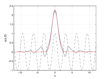
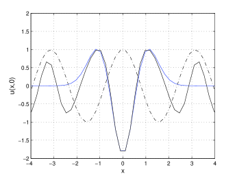
Figure 5: Comparison of profiles generated by the variational approximation for the stationary two-dimensional solitons based on the simple Gaussian ansatz (6) (red line), extended ansatz (12) (blue line), and direct numerical results (black line). The dashed-dotted curve shows the periodic potential. (a) A case intermediate between tightly- and loosely-bound solitons, corresponding to panel (e) in Fig. 4. (b) Zoom into the loosely-bound-soliton’s profile corresponding to panel (f) in Fig. 4 (in this case, the profile generated by the simple ansatz (6) is not included, as it is completely irrelevant).

References

- (1) N. K. Efremidis, S. Sears, D. N. Christodoulides, J. W. Fleischer, and M. Segev. Discrete solitons in photorefractive optically induced photonic lattices, Phys. Rev. E 66: 046602 (2002); N. K. Efremidis, J. Hudock, D. N. Christodoulides, J. W. Fleischer, O. Cohen, and M. Segev, Two-Dimensional Optical Lattice Solitons. Phys. Rev. Lett. 91: 213906 (2003).
- (2) J. W. Fleischer, T. Carmon, M. Segev, N. K. Efremidis, and D. N. Christodoulides. Observation of Discrete Solitons in Optically Induced Real Time Waveguide Arrays, Phys. Rev. Lett. 90: 023902 (2003); J. W. Fleischer, M. Segev, N. K. Efremidis, and D. N. Christodoulides. Observation of two-dimensional discrete solitons in optically induced nonlinear photonic lattices, Nature 422: 147-150 (2003).
- (3) D. N. Neshev, T. J. Alexander, E. A. Ostrovskaya, Y. S. Kivshar, H. Martin, I. Makasyuk, and Z. Chen. Observation of Discrete Vortex Solitons in Optically Induced Photonic Lattices, Phys. Rev. Lett. 92: 123903 (2004); J. W. Fleischer, G. Bartal, O. Cohen, O. Manela, M. Segev, J. Hudock, and D. N. Christodoulides. Observation of Vortex-Ring “Discrete” Solitons in 2D Photonic Lattices, Phys. Rev. Lett. 92: 123904 (2004).
- (4) B. B. Baizakov, B. A. Malomed and M. Salerno. Multidimensional solitons in periodic potentials, Europhys. Lett. 63: 642-648 (2003).
- (5) N. K. Efremidis, J. Hudock, D. N. Christodoulides, J. W. Fleischer, O. Cohen, and M. Segev. Two-Dimensional Optical Lattice Solitons, Phys. Rev. Lett. 91: 213906 (2003).
- (6) J. Yang and Z. H. Musslimani. Fundamental and vortex solitons in a two-dimensional optical lattice, Opt. Lett. 28: 2094-2096 (2003); Z. H. Musslimani and J. Yang. Self-trapping of light in a two-dimensional photonic lattice, J. Opt. Soc. Am. B 21: 973-981 (2004).
- (7) B. B. Baizakov, M. Salerno, and B. A. Malomed. Multidimensional solitons and vortices in periodic potentials. In: Nonlinear Waves: Classical and Quantum Aspects, ed. by F. Kh. Abdullaev and V. V. Konotop, pp. 61-80 (Kluwer Academic Publishers: Dordrecht, 2004); available online at http://rsphy2.anu.edu.au/~asd124/Baizakov_2004_61_NonlinearWaves.pdf.
- (8) B. B. Baizakov, B. A. Malomed and M. Salerno. Multidimensional solitons in a low-dimensional periodic potential, Phys. Rev. A 70, 053613 (2004).
- (9) L. Bergé. Wave collapse in physics: Principles and applications to light and plasma physics, Phys. Rep. 303: 259-372 (1998).
- (10) D. Mihalache, D. Mazilu, F. Lederer, Y. V. Kartashov, L.-C. Crasovan, and L. Torner. Stable three-dimensional spatiotemporal solitons in a two-dimensional photonic lattice, Phys. Rev. E 70: 055603(R) (2004).
- (11) Y. V. Kartashov, V. A. Vysloukh, and L. Torner. Rotary Solitons in Bessel Optical Lattices, Phys. Rev. Lett. 93: 093904 (2004).
- (12) D. Mihalache, D. Mazilu, F. Lederer, B. A. Malomed, Y. V. Kartashov, L.-C. Crasovan, and L. Torner. Stable spatiotemporal solitons in Bessel optical lattices, to be published.
- (13) C. J. Pethik and H. Smith, Bose-Einstein Condensation in Dilute Gases, Cambridge University Press, Cambridge, 2002.
- (14) B. B. Baizakov, V. V. Konotop and M. Salerno. Regular spatial structures in arrays of Bose–Einstein condensates induced by modulational instability, J. Phys. B: At. Mol. Opt. Phys. 35: 5105–5119 (2002).
- (15) E. A. Ostrovskaya and Yu. S. Kivshar. Matter-wave gap solitons in atomic band-gap structures, Phys. Rev. Lett. 90: 160407 (2003).
- (16) B. Eiermann, Th. Anker, M. Albiez, M. Taglieber, P. Treutlein, K.-P. Marzlin, and M. K. Oberthaler. Bright Bose-Einstein Gap Solitons of Atoms with Repulsive Interaction. Phys. Rev. Lett. 92: 230401 (2004).
- (17) H. Sakaguchi and B. A. Malomed, J. Phys. B: At. Mol. Opt. Phys. 37: 2225-2239 (2004).
- (18) E. A. Ostrovskaya and Yu. S. Kivshar. Photonic crystals for matter waves: Bose-Einstein condensates in optical lattices, Opt. Express 12: 19-29 (2004); Matter-Wave Gap Vortices in Optical Lattices, Phys. Rev. Lett. 93: 160405 (2004).
- (19) P. G. Kevrekidis, G. Theocharis, D. J. Frantzeskakis, and B. A. Malomed. Feshbach resonance management for Bose-Einstein condensates. Phys. Rev. Lett. 90: 230401 (2003).
- (20) F. Kh. Abdullaev, J. G. Caputo, R. A. Kraenkel, and B. A. Malomed. Controlling collapse in Bose-Einstein condensation by temporal modulation of the scattering length, Phys. Rev. A 67: 013605 (2003).
- (21) H. Saito and M. Ueda. Dynamically Stabilized Bright Solitons in a Two-Dimensional Bose-Einstein Condensate, Phys. Rev. Lett. 90: 040403 (2003).
- (22) G. D. Montesinos, V. M. Pérez-García, and P. J. Torres, Stabilization of solitons of the multidimensional nonlinear Schrödinger equation: matter-wave breathers, Physica D 191: 193-210 (2004).
- (23) I. Towers and B. A. Malomed. Stable (2+1)-dimensional solitons in a layered medium with sign-alternating Kerr nonlinearity, J. Opt. Soc. Am. B 19: 537-543 (2002).
- (24) M. Trippenbach, M. Matuszewski, and B. A. Malomed. Stabilization of three-dimensional matter-waves solitons in an optical lattice, Europhys. Lett., in press.
- (25) K. E. Strecker, G. B. Partridge, A. G. Truscott, and R. G. Hulet. Formation and propagation of matter-wave soliton trains, Nature 417: 150-153 (2002); L. Khaykovich, F. Schreck, G. Ferrari, T. Bourdel, J. Cubizolles, L. D. Carr, Y. Castin, and C. Salomon. Formation of a matter-wave bright soliton, Science 296: 1290-1293 (2002).
- (26) B. A. Malomed. Variational methods in nonlinear fiber optics and related fields, Progr. Optics 43: 71-193 (2002).
- (27) V. M. Pérez-García, H. Michinel, J. I. Cirac, M. Lewenstein, and P. Zoller. Low energy excitations of a Bose-Einstein condensate: A time-dependent variational analysis, Phys. Rev. Lett. 77: 5320-5326 (1996); Dynamics of Bose-Einstein condensates: Variational solutions of the Gross-Pitaevskii equations, Phys. Rev. A 56: 1424-1432 (1997).
- (28) B. B. Baizakov and M. Salerno. Delocalizing transition of multidimensional solitons in Bose-Einstein condensates, Phys. Rev. A 91: 213906 (2003).
- (29) G. Kalosakas, K. Ø. Rasmussen, and A. R. Bishop. Delocalizing Transition of Bose-Einstein Condensates in Optical Lattices, Phys. Rev. Lett. 89: 030402 (2002).
- (30) S. Darmanyan, A. Kobyakov, and F. Lederer. Stability of strongly localized excitations in discrete media with cubic nonlinearity, Zh. Eksp. Teor. Fiz. 113: 1253–1260 (1998) [JETP 86: 682-686 (1998)].
- (31) T. Kapitula, P. G. Kevrekidis, and B. A. Malomed. Stability of multiple pulses in discrete systems, Phys. Rev. E 63: 036604.
- (32) P. G. Kevrekidis, B. A. Malomed, and A. R. Bishop. Bound states of two-dimensional solitons in the discrete nonlinear Schrödinger equation, J. Phys. A Math. Gen. 34: 9615-9629 (2001).