Two-component gap solitons in two- and one-dimensional Bose-Einstein condensates

Abstract

We introduce two- and one-dimensional (2D and 1D) models of a binary BEC (Bose-Einstein condensate) in a periodic potential, with repulsive interactions. We chiefly consider the most fundamental case of the inter-species repulsion with zero intra-species interactions. The same system may also model a mixture of two mutually repulsive fermionic species. Existence and stability regions for gap solitons (GSs) supported by the interplay of the inter-species repulsion and periodic potential are identified. Two-component GSs are constructed by means of the variational approximation (VA) and in a numerical form. The VA provides accurate description for the GS which is a bound state of two tightly-bound components, each essentially trapped in one cell of the periodic potential. GSs of this type dominate in the case of intra-gap solitons, with both components belonging to the first finite bandgap of the linear spectrum (only this type of solitons is possible in a weak lattice). Inter-gap solitons, with one component residing in the second bandgap, and intra-gap solitons which have both components in the second gap, are possible in a deeper periodic potential, with the strength essentially exceeding the recoil energy of the atoms. Inter-gap solitons are, typically, bound states of one tightly- and one loosely-bound components. In this case, results are obtained in a numerical form. The number of atoms in experimentally relevant situations is estimated to be $\sim 5,000$ in 2D intra-gap soliton, and $\sim 25,000$ in its inter-gap counterpart; in 1D solitons, it may be up to $10^{5}$. For 2D solitons, the stability is identified in direct simulations, while in the 1D case it is done via eigenfrequencies of small perturbations, and then verified by simulations. In the latter case, if the intra-gap soliton in the first bandgap is weakly unstable, it evolves into a stable breather, while unstable solitons of other types (in particular, inter-gap solitons) get completely destroyed. The intra-gap 2D solitons in the first bandgap are less robust, and in some cases they are completely destroyed by the instability. Addition of intra-species repulsion to the repulsion between the components leads to further stabilization of the GSs.

I Introduction

Solitons in Bose-Einstein condensates (BECs) have drawn a great deal of attention as robust nonlinear matter-wave pulses. Bright (localized) solitons were first experimentally created in an effectively one-dimensional (1D) condensate of ⁷Li, loaded in a strongly elongated (nearly one-dimensional) “cigar-shaped” trap Li . The use of the Feshbach resonance (FR) made it possible to keep the scattering length in the condensate negative, with a very small absolute value, $\sim 0.1$ nm. The weak self-attractive nonlinearity controlled by means of this technique was sufficient to create 1D solitons, being a way below the collapse threshold in the cigar-shape configuration, thus securing the stability of the solitons.

More generic for BEC is a positive scattering length, corresponding to repulsive interactions between atoms. In this case, bright solitons may be created as a result of the interplay of the intrinsic repulsion and periodic potential induced by an optical lattice (OL, i.e., the interference pattern created by counterpropagating beams illuminating the condensate). It was predicted GS ; Ostrovskaya that gap solitons (GSs) may emerge in bandgaps of the system’s spectrum, since the interplay of a negative effective mass, appearing in a part of the gap, with the repulsive interaction is exactly what is needed to create a bright soliton. Theoretical models for GSs in BEC were reviewed in Ref. Konotop , and a rigorous stability analysis for them was developed in Ref. Pelinovsky . Experimentally, a GS in the ⁸⁷Rb condensate with a positive scattering length, loaded into a cigar-shaped trap equipped with a longitudinal OL, was for the first time created in Ref. Oberthaler (the soliton was composed of $\sim 1000$ atoms).

Binary mixtures of BECs are also available to experimental studies. Most typically, they contain two different hyperfine states of the same atomic species, such as ⁸⁷Rb Rb and ²³Na Na . BEC was also created in a heteronuclear mixture of ⁴¹K and ⁸⁷Rb hetero . As mentioned above, the magnitude and sign of the scattering lengths of collisions between atoms in the same species may be altered, via the FR technique, by an external spatially uniform magnetic Feshbach or optical optical-Feshbach field. The scattering length of collisions between atoms belonging to different species may also be controlled by the magnetic field inter-Feshbach .

The latter possibility opens a way to create a binary mixture with the (natural) intra-species repulsion, while the sign of the inter-species interaction is switched to attraction. In recent preprints symbiotic , it was proposed to use this possibility to create symbiotic bright solitons: while each self-repulsive species cannot support a soliton by itself, the inter-species attraction opens a way to make two-component solitons. A somewhat similar possibility was earlier proposed in terms of a Bose-Fermi mixture, where the interaction between bosons is repulsive, but the bosons and fermions attract each other Poland . Related to the latter setting, is a proposal to use attraction between fermions and bosons to built bosonic quantum dots for fermions (in particular, gap solitons in the BEC trapped in an OL may play the role of such quantum dots) Salerno .

In the present work, the aim to construct 2D and 1D solutions for two-component GSs in the most natural setting, when the inter-species interaction is repulsive. We will chiefly focus on the basic case, when intra-species interactions may be completely neglected, while the interplay of the OL potential and repulsion between the two species help to build GSs. The actual possibility to nullify the intra-species scattering length by means of the FR depends on the atomic species: as is known, it can be done in ⁷Li (see, e.g., Ref. FRlithium ), while in ⁸⁷Rb loss effects grow close to the FR point. Another possibility is offered by spinor condensates, where the scattering lengths which determine collisions between atoms with the same or opposite values of the hyperfine spin, $m_{F}=\pm 1$, can be represented, respectively, as Ho $a=a_{0}\pm a_{2}$, the coefficients $a_{0}$ and $a_{0}$ accounting for the mean-field (spin-independent) and spin-exchange interactions between the atoms. In this case, the self-scattering length vanishes in the case of $a_{2}=-a_{0}$.

Besides that, the model with zero interaction inside each species and repulsion between them may also apply to a mixture of two ultra-cold Fermi gases Poland ; Salerno . In this connection, it is relevant to mention that the scattering length of collisions between fermionic atoms (such as ⁶Li) may also be controlled by means of the FR FRlithium ; FRfermion . An effect of the intra-species repulsion will be briefly considered too, with a conclusion that it additionally stabilizes two-component GSs.

The periodic OL potential gives rise to many bandgaps in the system’s spectrum. In this work we concentrate on the most fundamental situations, with the two components of the soliton belonging to two lowest-order gaps. This way, we will demonstrate intra-gap solitons, with both components sitting in either the first or second gap, and inter-gap solitons, with the components belonging to the different (first and second) gaps.

The paper is structured as follows. The model is set in Section 2. An analytical variational approximation for 2D two-component solitons is presented in Section 3. Direct numerical results, that identify existence and stability regions of the intra- and inter-gap solitons, are reported in Section 3. The stability of the 2D solitons is investigated in direct simulations, which reveal not only stable stationary solitons, but stable breathers too. Basic results for the 1D version of the same two-component model are collected in Section 4; in particular, the stability of the 1D soliton is identified via computation of eigenvalues for small perturbations (which is more difficult in the 2D case). The paper is concluded by Section 6, where we also give estimates for actual numbers of atoms in the solitons predicted in this work.

II The model

In the mean-field approximation, the binary BEC at zero temperature is described by a system of two coupled Gross-Pitaevskii equations (GPEs) for the wave functions $\Psi(X,Y,Z;T)$ and $\Phi(X,Y,Z;T)$ of the two species Pethick :

$$i\hbar\frac{\partial\Psi}{\partial T} = -\frac{\hbar^{2}}{2m}\left(\frac{\partial^{2}\Psi}{\partial X^{2}}+\frac{\partial^{2}\Psi}{\partial Y^{2}}+\frac{\partial^{2}\Psi}{\partial Z^{2}}\right)$$

$$+V_{0}\left[\cos(2kX)+\cos(2kY)\right]\Psi+U(Z)\Psi+\frac{4\pi\hbar^{2}}{m}a\left(\rho|\Psi|^{2}+|\Phi|^{2}\right)\Psi,$$

$$i\hbar\frac{\partial\Phi}{\partial T} = -\frac{\hbar^{2}}{2m}\left(\frac{\partial^{2}\Phi}{\partial X^{2}}+\frac{\partial^{2}\Phi}{\partial Y^{2}}+\frac{\partial^{2}\Psi}{\partial Z^{2}}\right)$$

$$+V_{0}\left[\cos(2kX)+\cos(2kY)\right]\Phi+U(Z)\Phi+\frac{4\pi\hbar^{2}}{m}a\left(\rho|\Phi|^{2}+|\Psi|^{2}\right)\Phi,$$

where $m$ is mass of of both species of atoms, $V_{0}$ and $\pi/k$ are the amplitude and period of the OL potential, $U(Z)$ is a potential accounting for the tight magnetic or optical confinement in the transverse direction, that makes the condensate effectively two-dimensional (squeezing it into a “pancake” shape pancake ), while $a$ and $\rho a$ (with $\rho\geq 0$) are the scattering lengths of the inter-species and intra-species collisions. The equations do not include an external trapping potential in the $\left(X,Y\right)$ plane, as we are interested in localized 2D states supported intrinsically by the interplay of the inter-species repulsion and OL potential.

Assuming that the transverse trap gives rise to a ground-state wave function $\chi_{0}(Z)$ with the respective energy $E_{0}$, reduction of Eqs. (LABEL:GPE) to a normalized system of effective two-dimensional equations follows the usual procedure, based on averaging in the $Z$ direction and rescaling Pethick . To this end, we define $\left\{kX,kY\right\}\equiv\left\{x,y\right\},~{}\left(\hbar k^{2}/2m\right)T\equiv t,~{}2mV_{0}/\left(\hbar k\right)^{2}\equiv\varepsilon$ ($\varepsilon$ measures the ratio of the height of the OL’s potential barrier to the atom’s recoil energy), and

$$\left\{\Psi,\Phi\right\}\equiv e^{iE_{0}T/\hbar}\sqrt{\frac{\int_{-\infty}^{+\infty}\chi_{0}^{2}(Z)dZ}{\int_{-\infty}^{+\infty}\chi_{0}^{4}(Z)dZ}}\frac{k}{2\sqrt{2\pi a}}\left\{\psi(x,y;t),\phi(x,y;t)\right\}.$$ (2)

The eventual form of the 2D equations is

$$i\psi_{t}+\psi_{xx}+\psi_{yy}+\varepsilon\left[\cos(2x)+\cos(2y)\right]\psi-\left(\rho|\psi|^{2}+|\varphi|^{2}\right)\psi = 0,$$

$$i\varphi_{t}+\varphi_{xx}+\varphi_{yy}+\varepsilon\left[\cos(2x)+\cos(2y)\right]\varphi-\left(\rho|\varphi|^{2}+|\psi|^{2}\right)\varphi = 0.$$

In addition to $\varepsilon$ and $\rho$, control parameters of the normalized system are norms of both components,

$$N_{1}=\int\int\left|\psi(x,y)\right|^{2}dxdy,~{}N_{2}=\int\int\left|\varphi(x,y)\right|^{2}dxdy,$$ (4)

which determine the respective numbers of atoms as per Eq. (2):

$$\left(N_{\mathrm{phys}}\right)_{1,2}=\frac{1}{8\pi a}\frac{\left(\int_{-\infty}^{+\infty}\chi_{0}^{2}(Z)dZ\right)^{2}}{\int_{-\infty}^{+\infty}\chi_{0}^{4}(Z)dZ}N_{1,2}.$$ (5)

Norms (4), together with the Hamiltonian of the system, are its dynamical invariants. As said above, we will be mostly dealing with the case of $\rho=0$ (no intra-species interactions), hence essential parameters are $\varepsilon$ and $N_{1,2}$ (generally, we will consider the asymmetric case, with $N_{1}\neq N_{2}$).

Stationary solutions of Eqs. (LABEL:model) are looked for in the usual form,

$$\psi(x,y,t)=u(x,y)\exp(-i\mu_{1}t),~{}\varphi(x,y,t)=v(x,y)\exp(-i\mu_{2}t),$$ (6)

where $\mu_{1}$ and $\mu_{2}$ are real chemical potentials, and the real functions $u(x,y)$ and $v(x,y)$ are solutions of the equations

$$\mu_{1}u+u_{xx}+u_{yy}+\varepsilon\left[\cos(2x)+\cos(2y)\right]u-v^{2}u = 0,$$

$$\mu_{2}v+v_{xx}+v_{yy}+\varepsilon\left[\cos(2x)+\cos(2y)\right]v-u^{2}v = 0.$$

Linearization decouples Eqs. (LABEL:stationary_model), hence each chemical potential must belong to one of bandgaps of the 2D linear operator,

$$\hat{L}=\frac{\partial^{2}}{\partial x^{2}}+\frac{\partial^{2}}{\partial y^{2}}+\varepsilon\left[\cos(2x)+\cos(2y)\right]$$ (8)

(the spectrum of the operator is known, see, e.g., Ref. Ostrovskaya and Fig. 1 below). Note that $\mu_{1}$ and $\mu_{2}$ may be placed in different gaps, which gives rise, as said above, to two-component inter-gap solitons, as opposite to ones of the intra-gap type, with $\mu_{1}$ and $\mu_{2}$ belonging to the same bandgap. Below, we will demonstrate that the model supports stable solitons of both types (the consideration will actually be limited to two lowest gaps, the intra-gap solitons being possible in both of them).

It is relevant to mention that, in nonlinear optics, one-component 1D spatial solitons sitting in higher gaps were experimentally observed in arrays of waveguides with the Kerr (cubic) nonlinearity Silberberg . Then, 2D spatial single-component lattice solitons with embedded vorticity, belonging to the second gap, were created in a photorefractive material equipped with a 2D photonic lattice Moti . Moreover, in the latter case, two-component solitons composed of a fundamental soliton in the first gap and a vortex soliton in the second gap were also created. The most essential difference of the photorefractive media from BEC is the saturable character of the photorefractive nonlinearity.

III Variational approximation for two-dimensional solitons

It is known that 1D and 2D solitons generated by the GPE with the lattice potential (in the 2D case, the lattice may be either two-dimensional or quasi-one-dimensional BBB2 ) are naturally classified, in both cases of the attractive BBB2 ; BBB1 and repulsive Sakaguchi interaction, as tightly-bound (TB, alias single-cell) and loosely-bound (LB, alias multi-cell) ones. The solitons of the TB and LB types are essentially localized in one or several cells of the OL potential, respectively.

TB solitons, in the 1D and 2D geometry alike (including the case of the 2D equation with the quasi-1D lattice), may be accurately predicted by the variational approximation (VA) BBB2 ; BBB1 (this approximation was first applied to the GPE in Refs. firstVA ; a general review of the technique can be found in Ref. Progress ). For LB solitons, the VA may provide an adequate approximation for the soliton’s central lobe only, but not for the slowly decaying oscillatory tails OurPaper .

We start the analysis with application of the VA to Eqs. (LABEL:stationary_model). The Lagrangian from which the equations are derived is $L=\int\int\mathcal{L}dxdy$, with the density

$$\mathcal{L} = \mu_{1}u^{2}+\mu_{2}v^{2}-u_{x}^{2}-u_{y}^{2}-v_{x}^{2}-v_{y}^{2}$$ (9)

$$+\varepsilon\left[\cos(2x)+\cos(2y)\right](u^{2}+v^{2})-u^{2}v^{2}.$$

We approximate the TB solitons by a simple isotropic Gaussian ansatz,

$$u(x,y)=A\exp\left(-\frac{x^{2}+y^{2}}{2a^{2}}\right),~{}v(x,y)=B\exp\left(-\frac{x^{2}+y^{2}}{2b^{2}}\right).$$ (10)

The substitution of the ansatz in Eq. (9) and integration yield an effective Lagrangian,

$$L = \pi N_{2}\left(-\frac{1}{b^{2}}+2\varepsilon e^{-b^{2}}\right)+\pi N_{1}\left(-\frac{1}{a^{2}}+2\varepsilon e^{-a^{2}}\right)$$ (11)

$$-\frac{N_{1}N_{2}}{\pi\left(a^{2}+b^{2}\right)}+\mu_{1}N_{1}+\mu_{2}N_{2},$$

where the norms of the components, $N_{1}=\pi A^{2}a^{2}$ and $N_{2}=\pi B^{2}b^{2}$, are obtained by the substitution of the ansatz (10) in Eqs. (4). Below, we use, instead of $N_{1}$ and $N_{2}$, the total and relative norms,

$$N\equiv N_{1}+N_{2},~{}N_{r}\equiv N_{1}/N_{2}$$ (12)

(we define $N_{1}$ and $N_{2}$ as the smaller and larger norms, respectively, hence $N_{r}\leq 1$).

The variational equations, $\partial L/\partial N_{1,2}=\partial L/\partial a=\partial L/\partial b=0$, applied to Lagrangian (11), yield the following relations that determine parameters of the soliton within the framework of the VA:

$$N_{r} = \frac{a^{4}}{b^{4}}\frac{1-2\varepsilon b^{4}e^{-b^{2}}}{1-2\varepsilon a^{4}e^{-a^{2}}},$$ (13)

$$N = \pi\left(1+\frac{b^{2}}{a^{2}}\right)^{2}(1+N_{r})\left(2\varepsilon a^{4}e^{-a^{2}}-1\right),$$ (14)

$$\mu_{1} = -\frac{b^{2}}{a^{4}}+2\left(a^{2}+b^{2}-1\right)\varepsilon e^{-a^{2}},$$ (15)

$$\mu_{2} = -\frac{a^{2}}{b^{4}}+2\left(a^{2}+b^{2}-1\right)\varepsilon e^{-b^{2}}.$$ (16)

Equations (13) and (14) give rise to necessary conditions for the existence of the soliton, $1-2\varepsilon a^{4}e^{-a^{2}}<0$ and $1-2\varepsilon b^{4}e^{-b^{2}}<0$, from which, in turn, it follows that that the GS does not exist unless the OL strength $\varepsilon$ exceeds a minimum (threshold) value, $\varepsilon_{\min}>e^{2}/8\approx 0.92$. The same condition for the existence of GSs was predicted by the VA in the single-component 2D model OurPaper .

The VA does not include information about the location of bandgaps in the system’s spectrum, therefore it is necessary to check whether the GSs predicted by the VA fall into the bandgaps. This is shown in Fig. 1, which demonstrates that the variational equations (13), (14) and (15), (16) for the symmetric GSs ($\mu_{1}=\mu_{2}\equiv\mu$) predict the boundary of the first finite gap (the lower bold dashed line) with surprisingly good accuracy. The accuracy may be explained by the fact that the Gaussian ansatz (10) provides for a good fit to the actual shape of the GS in the first finite gap (this, in particular, means that the VA correctly predicts the absence of solitons in the semi-infinite gap – the lowest one in Fig. 1, which extends to $\mu\rightarrow-\infty$). On the other hand, the correlation between the other VA-predicted soliton-existence boundary (the upper bold dashed line in Fig. 1) and the exact border of the bandgaps is very crude, due to the fact that the GSs in higher gaps are very different from the simple ansatz OurPaper .

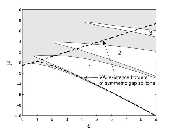
Figure 1: The region of the existence of symmetric gap solitons (the area between the two bold dashed lines), as predicted by the variational approximation based on the Gaussian ansatz (10), and the exact bandgap structure in the two-dimensional system. Shaded and unshaded regions are, respectively, the Bloch bands (where solitons cannot exist) and gaps (where solitons are possible), the numbers $1$, $2$, $3$ being numbers of the finite bandgaps. The lower unshaded region is the semi-infinite gap.

For the description of experimentally relevant situations, Fig. 2 displays the predicted GS existence regions in the plane of the total and relative soliton norms, $\left(N,N_{r}\right)$ [see the definitions in Eqs. (12)], which includes the general asymmetric solutions with $N_{r}<1$. False parts of the existence regions, that have either $\mu_{1}$ or $\mu_{2}$ falling into a Bloch band (rather than into a gap), are excluded in panels (b)-(d).

We note that, for relatively small $\varepsilon$ (however, it must exceed the above-mentioned threshold value $\varepsilon_{\min}$ necessary for the existence of the solitons), the VA predicts only intra-gap solutions, with both $\mu_{1,2}$ lying in the first finite gap. This prediction is correct, as for these values of $\varepsilon$ the spectrum of the two-dimensional GPE with the OL potential has only one finite gap, see Fig. 1. For larger $\varepsilon$, the VA predicts intra-gap solutions in the second gap, as well as inter-gap solitons, with the components belonging to the different finite bandgaps, first and second. With the further increase of $\varepsilon$, the regions of the intra-gap solutions in the first and second bandgaps and inter-gap solitons grow and overlap.

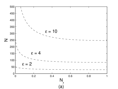
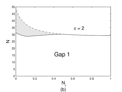
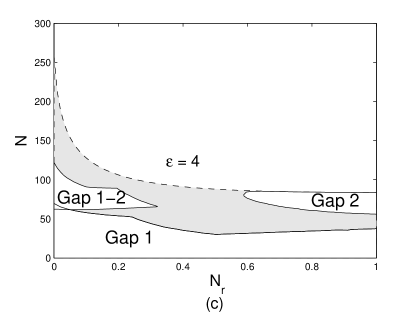
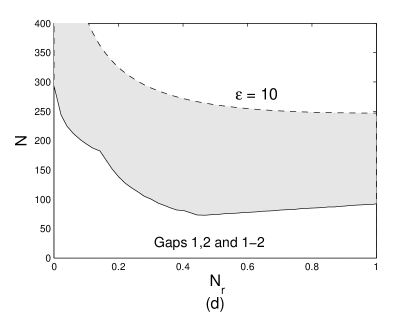
Figure 2: (a) The existence regions for the gap solitons in the ($N$,$N_{r}$) plane, as predicted (below the respective dashed lines) by the variational approximation for different values of the strength $\varepsilon$ of the optical lattice. Panels (b)-(d), which pertain, respectively, to $\varepsilon=2$,$~{}4$, and $10$, show that shaded portions of the predicted existence regions must be excluded, as in these areas either chemical potential, $\mu_{1}$ or $\mu_{2}$, falls into a Bloch band. The remaining white portions of the existence region in each panel are true ones, with both $\mu_{1}$ and $\mu_{2}$ located in one of the two lowest bandgaps. In panels (b) and (c), the bandgap(s) to which the chemical potentials belong are indicated. In panel (d), details for different gaps are not shown, because of a complex picture of areas corresponding to each gap.

IV Numerical results for two-dimensional solitons

IV.1 Families of intra- and inter-gap solitons

Comparison with numerically found stationary solutions for the GSs demonstrates that (as mentioned above) the applicability of the VA is indeed limited to strongly confined TB solitons. In most cases, the solitons with both components belonging to the first finite gap appertain to this type, and they are predicted by the VA very accurately, as shown in Fig. 3. Note, however, that strongly asymmetric intra-gap solitons cannot be found numerically in the first bandgap for values of the relative norm smaller than $\left(N_{r}\right)_{\min}\approx 0.05$. Nevertheless, the VA predicts asymmetric solitons for $N_{r}<\left(N_{r}\right)_{\min}$, up to $N_{r}=0$. The latter is an obvious artifact of the VA, as in the case of $N_{r}=0$ one component is empty $(\psi\equiv 0$), which makes the remaining equation linear, hence it cannot give rise to any soliton.

On the contrary to the situation for the intra-gap solitons belonging to the first finite bandgap, the prediction produced by the VA for the solitons with both components sitting in the second bandgap are completely wrong: as seen in the top panel of Fig. 3, the formally predicted family of the intra-gap solitons in the second gap has no numerically found counterpart.

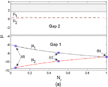
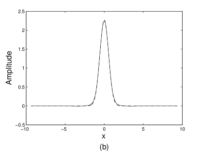
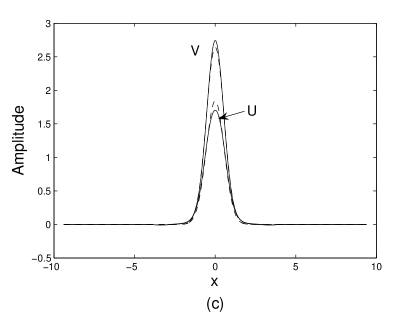
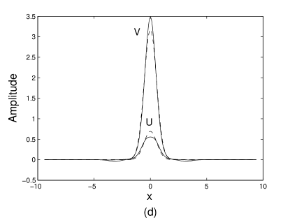
Figure 3: (Color online) Comparison of the variational approximation and numerical solutions for two-dimensional gap solitons in the case of $\varepsilon=10$, with the total norm $N=10$. The soliton families, as predicted by the VA and found in the numerical form, are shown by dashed and solid lines, respectively, in panel (a). In this panel, areas occupied by the Bloch bands (where solitons cannot exist), are shaded. Small circles (o) and crosses (x) designate, respectively, variational and numerical solutions that are displayed, as examples, in the remaining part of the figure: (b) $N_{r}=1$ (a symmetric soliton); (c) $N_{r}=0.5$; (d) $N_{r}=0.05$. In these panels, and in examples of the two-dimensional solitons presented below, their cross-sections along $y=0$ are displayed.

Increase of the total norm $N$ pushes the solution to the higher (second) bandgap. Figure 4 compares the numerical results and VA for such a situation (with $N$ five times as large as in Fig. 3). We observe that, while the VA is good for the symmetric solitons ($N_{r}=1$), it fails for more general asymmetric solutions – both intra-gap solitons belonging to the second gap, and inter-gap ones.

Figure 4 also shows that, as the asymmetry coefficient $N_{r}$ gets smaller, the soliton’s component with the smaller norm loses its single-peaked shape, see panels (c)-(e). We stress that no intra-gap soliton belonging to the second gap could be found (numerically) for $N_{r}<0.75$. The latter is seen in Fig. 4, where the branches corresponding to the intra-gap solution family terminate at $N_{r}\approx 0.75$.

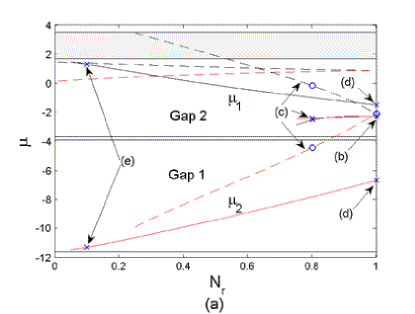
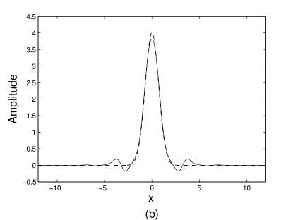
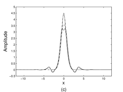
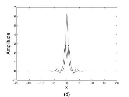
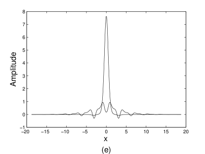
Figure 4: (Color online) The same as in the previous figure, but for $N=50$. Panels (b) and (c): examples of the intra-gap solitons, for $N_{r}=1$ and $N_{r}=0.8$, respectively, which belong to the second bandgap. Panels (d) and (e): examples of inter-gap solitons, with $N_{r}=1$ and $N_{r}=0.1$, respectively [in both these cases, the loosely-bound component belongs to the second (upper) bandgap, and in the latter case ($N_{r}=0.1$) the larger norm is in the first (lower) bandgap]. Note that the inter-gap soliton with $N_{r}=1$ is not a symmetric one, even if the norms of its two components are equal.

The findings presented in Fig. 4 include inter-gap solitons [in panels (d) and (e)], with $\mu_{2}$ in the first gap and $\mu_{1}$ in the second. As seen from panel (a) in the figure, these solitons could not be predicted by the VA. This is explained by the fact that at least one component of the inter-gap soliton has a loosely-bound shape, hence the Gaussian ansatz (10) is irrelevant for it. A typical example of the inter-gap soliton built as a TB-LB bound pair is shown in Fig. 5, for a still larger total norm, $N=70$. As well as in the above examples, the TB and LB components reside in the lower and upper gaps, respectively.

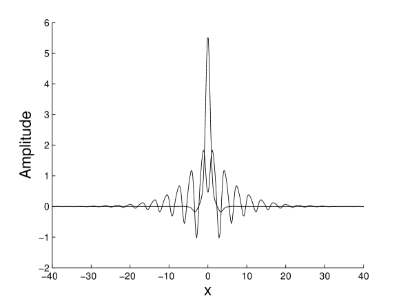
Figure 5: An example of an inter-gap soliton, built as a bound state of tightly- and loosely bound components with equal norms ($N_{r}=1$), for $\varepsilon=4$ and $N=70$. The corresponding chemical potentials are $\mu_{1}=$ $-1.64$ and $\mu_{2}=$ $3.3$.

Intra-gap solitons may also be TB-LB bound states. Figure 6 demonstrates how a symmetric TB soliton (with $N_{r}=1$) transforms into a TB-LB pair with the decrease of $N_{r}$, this time (on the contrary to the above examples of the inter-gap TB-LB bound states) the LB component having a larger norm, which is, in fact, a rule for asymmetric intra-gap solitons, as evidenced by our numerical results obtained with other values of the parameters.

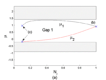
Figure 6: (Color online) Stable intra-gap solitons numerically found for $\varepsilon=2$ (in this case, the system’s spectrum contains only the first finite bandgap), with the total norm $N=20$. (a) The family of the gap-soliton solutions. (b) A tightly-bound symmetric soliton with $N_{r}=1$. (c) An example of a strongly asymmetric soliton, with $N_{r}=0.1$, in the form a bound state of loosely- and tightly bound components, with the larger norm sitting in the loosely-bound component.

With even larger norms (for instance, $N=150$), intra-gap solitons in the form of LB-LB bound pairs with very slowly decaying tails were found too, for $N_{r}>0.85$, i.e., they are nearly symmetric states. However, such solitons are unstable.

IV.2 Global existence and stability diagrams for the solitons

Results of systematic investigation of the existence and stability of the two-component two-dimensional GSs are summarized in Fig. 7, which is a typical example for the weak OL, with $\varepsilon=2$, that supports only one finite bandgap in the spectrum of the 2D model, and in Fig. 8, which represents relatively strong OLs (it has $\varepsilon=10$, which admits two distinct finite bandgaps).

Figure 7 shows that the entire gap is populated with solitons which are stable, except when both chemical potentials $\mu_{1}$ and $\mu_{2}$ are close to either the lower or upper bandgap edge. The stability was verified by direct simulations of the underlying GPEs (LABEL:model), with an initial perturbation imposed on the soliton by dislocating centers of its two components (simulations were performed by means of the split-step algorithm combined with the 2D fast Fourier transform). The dislocation leads to oscillatory dynamics, and GSs were classified as stable ones if they would oscillate near the initial shape. A caveat is that such a definition of the stability does not make a clear distinction between stable stationary solitons and stable breathers with a small amplitude of internal vibrations; however, the objects of both types are, as  a matter of fact, experimentally equivalent localized states in the BEC.

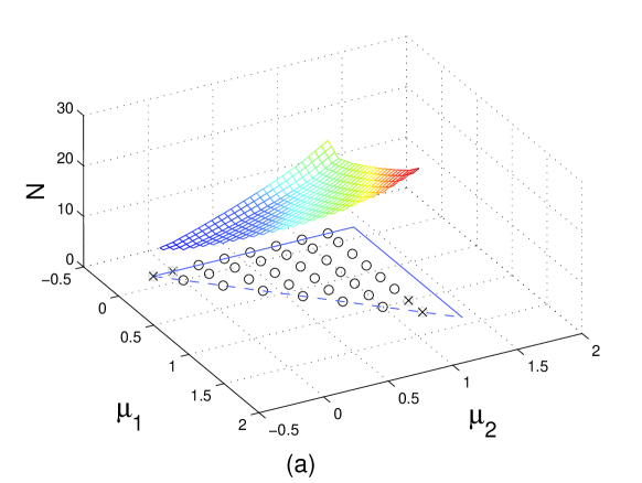
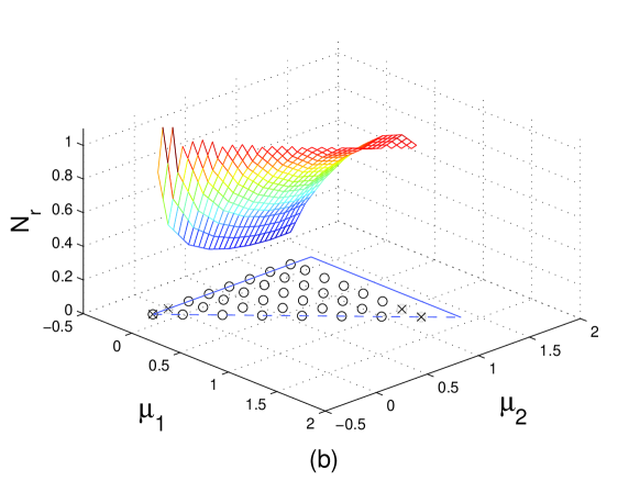
Figure 7: (Color online) The global existence and stability diagram for the two-component intra-gap solitons in the weak two-dimensional lattice potential, with $\varepsilon=2$ (the spectrum of the 2D Gross-Pitaevskii equation contains only one finite bandgap in this case). The total norm of the soliton, $N=N_{1}+N_{2}$, (a), and the relative norm, $N_{r}=N_{1}/N_{2}$, (b), are shown vs. the chemical potentials of the two components, $\mu_{1}$ and $\mu_{2}$. Solid lines in the $\left(\mu_{1},\mu_{2}\right)$ plane are the bandgap’s borders, and the dashed diagonal is the symmetry axis, $\mu_{1}=\mu_{2}$ (the identical mirror-image region on the other side of the diagonal is not shown). Stable and unstable solitons are designated, respectively, by small circles (o) and crosses (x).

Figure 8 shows that the stability pattern is more complex for a stronger OL, with $\varepsilon=10$. In particular, the inter-gap soliton, which is possible in this case, may be stable when the chemical potential $\mu_{1}$ of the component with a smaller norm, which appertains to the first (lower) bandgap, is sufficiently close to the lower edge of the gap. It is noteworthy that the stability region of the inter-gap solitons is found at values of the total norm $N$ at which intra-gap solitons, with both components sitting in the first bandgap, do not exist, i.e., there is no overlap between these two types of the stable GSs .

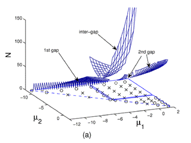
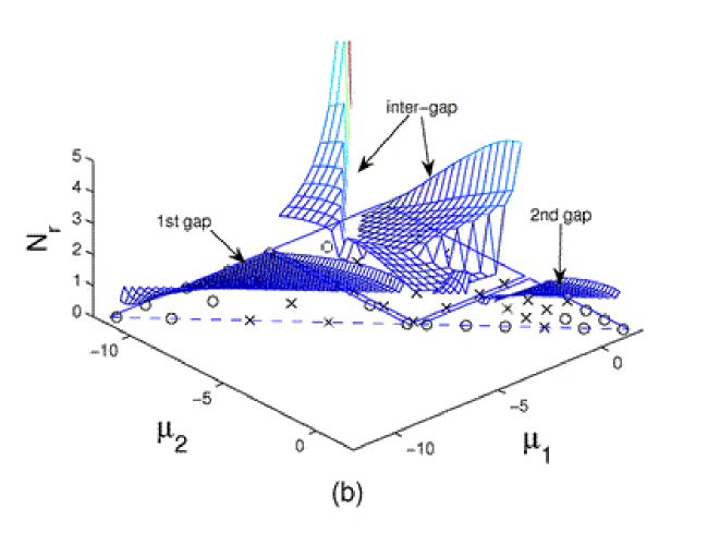
Figure 8: (Color online) The existence and stability diagram for the two-component gap solitons in a relatively strong lattice, with $\varepsilon=10$ (in this case, the 2D Gross-Pitaevskii equation gives rise to two finite bandgaps, therefore the diagram includes the family of inter-gap solitons). The notation is the same as in the previous figure, with labels additionally indicating the type of the solitons on each disjoint solution surface (labels “1st gap” and “2nd gap” pertain to intra-gap solitons belonging to the respective gaps). Double solid lines separating the bandgaps represent narrow Bloch bands between the gaps.

Further simulations demonstrate that unstable inter-gap solitons are either completely destroyed or evolve into symmetric solitons with both components belonging to the first gap. An example of such evolution is displayed in Fig. 9. In this case, the LB component of the TB-LB pair emits radiation until only the central lobe remains in it, and the whole structure turns into a symmetric intra-gap soliton of the TB type.

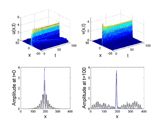
Figure 9: (Color online) Evolution of an unstable two-dimensional inter-gap soliton with $\mu_{1}=-3.7$, $\mu_{2}=-5.6$ is shown in the cross-section along the $y=0$ axis for $\varepsilon=10$. The loosely-bound component reduces its norm through emission of radiation. Eventually, the solution evolves into a symmetric intra-gap soliton of the tightly-bound type.

A specific instability mode was observed in unstable inter-gap solitons, as well as in intra-gap ones with both components belonging to the second gap, in the case when the unperturbed soliton features a single peak in one component and a double (split-tip) peak in the other. In this configuration, the instability triggers oscillatory dynamics with the single peak jumping irregularly between positions close to the two side peaks of the mate component. An example of this instability is displayed in Fig. 10. Further evolution leads to complete destruction of both components in this case.

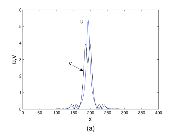
Figure 10: (Color online) The onset of the “jumping” instability of the two-dimensional intra-gap soliton with $\mu_{1}=0.5$ and $\mu_{2}=-2.5$, which belongs to the second bandgap, for $\varepsilon=10$. The upper panel shows the unperturbed shape of the soliton in the $y=0$ cross section, and the lower panels display, by means of contour plots, the evolution of both components in the same cross section.

Finally, simulations of the full model (LABEL:model) with $\rho\neq 0$, which includes the self-repulsion in each component, reveal a clear trend to stabilization of the two-component GSs as $\rho$ increases (of course, the model with $\rho>0$ gives rise to ordinary single-component GSs too). For example, the unstable symmetric soliton with $\mu_{1}=\mu_{2}=1.2$, $\varepsilon=2$, and $\rho=0$ (recall the system has a single finite bandgap in this case) becomes stable as the self-repulsion coefficient increases to $\rho_{\min}\approx 2/3$. This stabilization mechanism will be considered in more detail below in the 1D version of the model.

V One-dimensional solitons

The 1D variant of the model corresponds to a “cigar-shaped” binary condensate, tightly confined in the transverse plane, with a one-dimensional OL created in the longitudinal direction, $x$. The accordingly modified 1D version of the normalized equations (LABEL:model) is

$$i\psi_{t}+\psi_{xx}+\varepsilon\cos(2x)\psi-\left(\rho|\psi|^{2}+|\varphi|^{2}\right)\psi = 0,$$

$$i\varphi_{t}+\varphi_{xx}+\varepsilon\cos(2x)\varphi-\left(\rho|\varphi|^{2}+|\psi|^{2}\right)\varphi = 0.$$

The conserved norms of the scaled wave functions are

$$N_{1,2}\equiv\int_{-\infty}^{+\infty}\left\{\left|\psi(x)\right|^{2},\left|\varphi(x)\right|^{2}\right\}dx,$$ (18)

which are related to the numbers of atoms as follows:

$$\left(N_{\mathrm{phys}}\right)_{1,2}=\frac{k}{4a}\frac{\left(\int_{0}^{\infty}\chi_{0}^{2}(R)RdR\right)^{2}}{\int_{0}^{\infty}\chi_{0}^{4}(R)RdR}N_{1,2},$$ (19)

cf. Eq. (5). Here $\pi/k$ is, as above, the OL period, and $\chi_{0}(R)$ is the ground-state wave function of the tight confining potential, $R$ being the radial coordinate in the transverse plane.

A principal difference of the 1D model from its 2D counterpart is that, at any finite $\varepsilon$, the 1D version of the operator (8), which is the same as in the Mathieu equation, gives rise to an infinite system of finite bandgaps (recall that the 2D operator generates a single finite gap for small $\varepsilon$, two gaps for larger $\varepsilon$, etc.).

Stationary soliton solutions to Eqs. (LABEL:model1D) are again looked for in the form of Eqs. (6) (with the coordinate $y$ dropped). In contrast to the above analysis of the 2D model, in the present case we determine the stability of solitons in a rigorous way, from linearized equations for small perturbations about the stationary soliton (however, in all the cases when GSs were predicted to be stable in this sense, their stability was also verified in direct simulations). The application of the rigorous approach to the 2D model is to be presented elsewhere, as it is a technically involved problem.

The perturbed solutions are taken as

$$\psi = \left[u(x)+\psi_{1}(x)e^{-i\lambda t}\right]e^{-i\mu_{1}t},$$

$$\varphi = \left[v(x)+\varphi_{1}(x)e^{-i\lambda t}\right]e^{-i\mu_{2}t},$$

where $\psi_{1}$ and $\varphi_{1}$ are eigenmodes of infinitesimal perturbations and $\lambda$ is the respective eigenfrequency, the instability corresponding to having $\mathrm{Im~{}}\lambda>0$. The substitution of this in Eqs. (LABEL:model1D) and linearization lead to the equations

$$\left(\mu_{2}+\frac{d^{2}}{dx^{2}}\right)\psi_{1}+\varepsilon\cos(2x)\psi_{1}-\left[v^{2}(x)\psi_{1}+u(x)v(x)\left(\phi_{1}+\phi_{1}^{\ast}\right)\right]$$

$$-\rho u^{2}(x)\left(2\psi_{1}+\psi_{1}^{\ast}\right) = \lambda\psi_{1},$$

$$\left(\mu_{1}+\frac{d^{2}}{dx^{2}}\right)\phi_{1}+\varepsilon\cos(2x)\phi_{1}-\left[u^{2}(x)\phi_{1}+u(x)v(x)\left(\psi_{1}+\psi_{1}^{\ast}\right)\right]$$

$$-\rho v^{2}(x)\left(2\phi_{1}+\phi_{1}^{\ast}\right) = \lambda\phi_{1},$$

which can be solved by means of known numerical methods, to yield a full spectrum of the eigenfrequencies $\lambda$ (we used the Matlab eigenvalue-finding routine; it is based on approximating the ordinary differential equations by a system of linear homogeneous algebraic equations, computing the determinant of the corresponding matrix, and equating it to zero, which eventually leads to an equation for $\lambda$).

First of all, we present results for the most fundamental case of $\rho=0$, when only two-component GSs are possible, as well as in the 2D model considered above. Fixing the OL strength $\varepsilon$, in Figs. 11(a) and (b) we display the total and relative norms, $N$ and $N_{r}$ for the family of 1D two-component GSs, as functions of the two chemical potentials, $\mu_{1}$ and $\mu_{2}$, for a case when both belong to the first finite bandgap (i.e., for the family of intra-gap solitons) [the norms $N$ and $N_{r}$ are defined as in Eqs. (12), with $N_{1}$ and $N_{2}$ taken as per Eq. (18)]. The stability of the same GS family is presented in panel (c) of Fig. 11, which shows the largest value of $\mathrm{Im~{}}\lambda$, i.e., the instability growth rate, as a function of $\mu_{1}$ and $\mu_{2}$ [the border between stable and unstable solitons is indicated in Figs. 11(a) and (b) too]. If the GS of this type is unstable, its instability is oscillatory (i.e., $\mathrm{Im~{}}\lambda>0$ comes along with $\mathrm{Re~{}}\lambda\neq 0$). Typically, the instability does not destroy the soliton, but rather transforms it into quite a stable breather, see an example in Fig. 11(d).

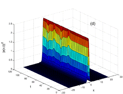
Figure 11: (Color online) A typical example of a family of two-component intra-gap solitons in the one-dimensional model, with both components belonging to the first finite bandgap. In this case, $\varepsilon=8$ (and $\rho=0$). Panels (a), (b), and (c) show, respectively, the total norm $N=N_{1}+N_{2}$, relative norm $N_{r}=N_{1}/N_{2}$, and instability growth rate, $\mathrm{Im~{}}\lambda$. Panel (d) displays an example of the transformation of an unstable symmetric intra-gap soliton (with $\mu_{1}=\mu_{2}=0$) into a stable breather, due to the oscillatory instability.

Inter-gap solitons, built of components belonging to the fist and second finite bandgaps, have also been investigated in detail in the 1D model. Characteristics of this solution family are presented in Fig. 12. As seen from panel (c) of the figure, the stability area of the inter-gap solitons is essentially smaller than in the case of their intra-gap counterparts, cf. Fig. 11(c). Note that panels (a), (b) and (c) in Fig. 12 do not show a Bloch band that separates the two gaps (unlike Fig. 8 in the 2D model), as the ranges of values on the axes of $\mu_{1}$ and $\mu_{2}$ in these panels cover, respectively, only the first and second gaps.

It is noteworthy that, as well as in the 2D model, the inter-gap solitons are bound states of TB and LB components belonging to the first and second gaps, respectively. An example of a stable inter-gap soliton that clearly demonstrates this structure is shown in Fig. 12(d) [cf. Figs. 4(d) and (e) and Fig. 5, which display cross sections of intra-gap solitons in the 2D model].

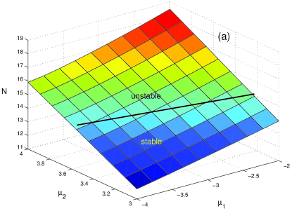
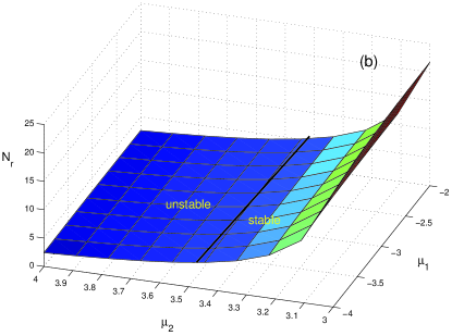
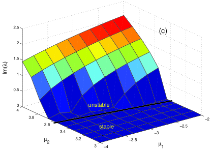
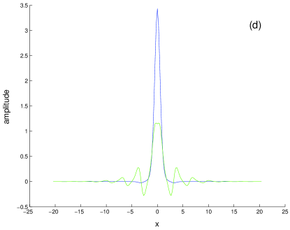
Figure 12: (Color online) Panels (a), (b), and (c) show the same characteristics as in Fig. 11 for a typical family of two-component inter-gap solitons in the one-dimensional model, with one component belonging to the first finite bandgap, and the other – to the second. In this case, $\varepsilon=8$ and $\rho=0$. Panel (d) displays a generic example of a stable inter-gap soliton, with $\mu_{1}=-3$, $N_{1}=11.7$, and $\mu_{2}=3$, $N_{2}=0.75$.

If an inter-gap soliton is unstable, its instability again has the oscillatory character. However, the action of the instability on the inter-gap soliton is more destructive than it was in the case of its intra-gap counterpart: instead of transforming the stationary soliton into a well-localized breather [see Fig. 11(d)], the instability triggers much more violent evolution, as illustrated by a typical example in Fig. 13.

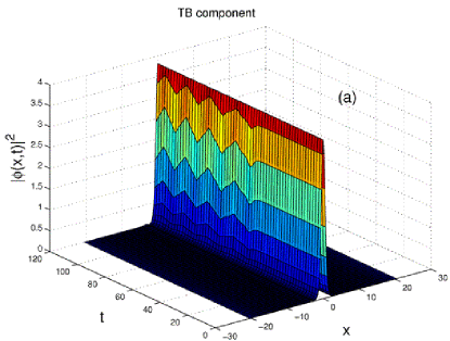
Figure 13: (Color online) An example of the evolution of an unstable inter-gap soliton in the one-dimensional model with $\varepsilon=8$, $\rho=0$ and $\mu_{1}=-3$, $\mu_{2}=4$. Panels (a) and (b) show the development of the instability in the components that originally belong to the first and second finite gaps, respectively.

One-dimensional intra-gap solitons belonging to the second gap were constructed and investigated too, with a conclusion that they all are unstable, although the instability growth rate may sometimes be very small. An example illustrating the instability of this species of the GS is displayed in Fig. 14. This conclusion seems to be in contrast with results reported above for the 2D model, where a small stability area for the intra-gap solitons appertaining to the second finite bandgap was found, see Fig. 8. However, the stability of the 2D solitons was identified not via eigenfrequencies of small perturbations, but rather by means of direct simulations, and the numerical stability test always turned the stationary soliton into a weakly excited state (a breather with a small amplitude of intrinsic vibrations). Therefore (as it was said above), in the 2D case we, strictly speaking, cannot tell a difference between a weakly unstable stationary soliton and a weakly excited stable breather into which the dynamical evolution may transform the unstable soliton. Thus, it may happen that what was identified as stable 2D intra-gap solitons sitting in the second finite bandgap are, actually, stable breathers with a small vibration amplitude, similar to what is observed in Fig. 11(d).

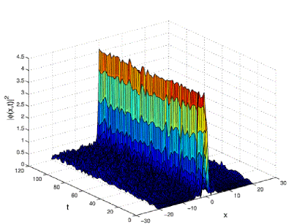
Figure 14: (Color online) Instability of a symmetric intra-gap soliton appertaining to the second finite bandgap in the one-dimensional model. In this case, $\varepsilon=8$, $\rho=0$ and $\mu=4$.

We have also investigated in some detail the effect of the self-repulsion term in the full 1D system (LABEL:model1D). As was already mentioned above in connection to the 2D model, the increase of the self-repulsion coefficient $\rho$ leads to stabilization of the GSs. A similar effect in the 1D setting is clearly seen in Fig. 15. It demonstrates that a stable symmetric intra-gap soliton belonging to the second finite bandgap, which, as said above, is always unstable in the 1D model with $\rho=0$, becomes stable if $\rho$ exceeds a minimum (threshold) value, which, in this case, is $\rho_{\min}\approx 0.9$.

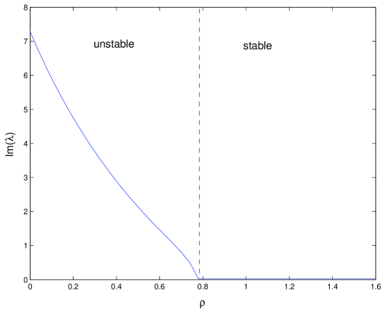
Figure 15: (Color online) The instability growth rate of a symmetric soliton in the second finite bandgap vs. the self-repulsion coefficient $\rho$ [see Eqs. (LABEL:model1D)]. Except for $\rho$, parameters are the same as in the previous figure. The soliton is stable in the region of $\rho>\rho_{\min}\approx 0.8$.

The above stability analysis was performed within the framework of the GPE, i.e., in the mean-field approximation at zero temperature. A physically important issue is stability of the same solitons against quantum and thermal fluctuations beyond the framework of the mean-field theory. The interest to this issue is enhanced by experimental observation of quite strong effective re-thermalization the ultra-cold condensate under the action of the OL potential thermo . To extend the analysis in this direction, one may use a system of self-consistent time-dependent Hartree-Fock-Bogoliubov (TDHFB) equations, built around the corresponding Gross-Pitaevskii equation(s) TDHFB . This approach was recently used to demonstrate possible instability of an ordinary 1D soliton (not of the gap type) in the BEC with attractive interactions, which is completely stable in the framework of the GPE proper MotiAvi . In that case, the instability splits the soliton into two segments.

A properly modified system of the TDHFB equations (including the OL potential and repulsive inter-species interaction) can also be used for the investigation of the extended stability of the two-component GSs studied in this work. We have performed a preliminary analysis along these lines, and concluded that those 1D solitons which are stable within the framework of Eqs. (LABEL:model1D) are also stable (at least, in most cases) against fluctuations governed by the TDHFB equations. A systematic consideration of this issue, especially for the 2D model, requires a considerable amount of additional work and will be reported elsewhere.

VI Conclusion

In this work, we have introduced a model of a binary BEC with intrinsic inter- and intra-species repulsion (positive scattering lengths), which is loaded into the periodic optical-lattice potential. Both two- and one-dimensional versions of the model were considered. We focused on the most fundamental case (different from previously studied models), with repulsion between the two species and zero intra-species interaction, which can be achieved by means of the Feshbach-resonance (FR) technique, or in a spinor condensate. The same system may also model a mixture of two mutually repulsive fermionic species.

The main problem was the existence and stability of gap solitons (GSs) supported by the interplay of the inter-species repulsion and periodic potential. Two-component GSs were looked for by means of the variational approximation (VA) and in the numerical form. It was found that the VA provides for good accuracy in the case when the 2D soliton is a bound state of two tightly-bound components, each being essentially confined around one cell of the periodic potential. Such a GS structure dominates in the case when both components belong to the first finite bandgap of the system’s spectrum (the intra-gap soliton). In fact, only this type of the GS is possible in a weak 2D lattice potential. On the contrary, inter-gap solitons, and intra-gap ones residing in the second finite bandgap (both types are possible in a stronger lattice potential, with the barrier height essentially larger than the recoil energy) are, typically, bound states of tightly- and loosely-bound components. For such structures, the VA is irrelevant, but general results were obtained in the numerical form, which made it possible to identify the existence and stability regions for the inter- and intra-gap solitons in both the 2D and 1D models. In the 2D case, the stability was tested in direct simulations, while in the 1D model the stability was identified in a rigorous way, through the computation of eigenfrequencies of small perturbations (the results were also verified by direct simulations). In the case when the 1D intra-gap soliton belonging to the first gap is weakly unstable, it evolves into a stable breather with a small amplitude of intrinsic vibrations. In contrast to this, if the 2D solitons in the first gap are unstable, they are completely destroyed by the instability. The same pertains to unstable 1D and 2D solitons of other types, such as inter-gap solitons, and intra-gap ones belonging to the second finite bandgap. It was also shown that introduction of the intra-species repulsion, in addition to the repulsion between the components, leads to further stabilization of solitons. In particular, some originally unstable types (such as 1D intra-gap solitons in the second bandgap) may be made stable, provided that the self-repulsion coefficient exceeds a certain minimum value. Preliminary analysis shows that the two-component GSs introduced in this work are stable too against fluctuations obeying the Hartree-Fock-Bogoliubov equations.

The actual number of atoms in the 2D solitons considered above, which is their most important physical characteristic, can be easily estimated. Undoing renormalizations which led to the 2D Gross-Pitaevskii equations in the form of Eqs. (LABEL:model) and making use of Eq. (5), one can derive the following relations between the density of atoms in physical units, $n_{\mathrm{phys}}$, and the rescaled one $|\psi|^{2}$, and between the number of atoms and the soliton’s norm:

$$n_{\mathrm{phys}}=\frac{\pi}{2a_{s}\Lambda^{2}}|\psi|^{2},~{}N_{\mathrm{phys}}=\frac{l_{z}}{8\pi a_{s}}N,$$ (21)

where $\Lambda$ is the period of the optical lattice, $a_{s}$ the scattering length of the inter-species collisions, and $l_{z}$ the size of the condensate in the transverse ($z$) direction (note that the relation between $N_{\mathrm{phys}}$ and $N$ does not contain $\Lambda$). Assuming experimentally reasonable values, $a_{s}\sim 1$ nm and $l_{z}\simeq 2$ $\mu$m (the latter pertains to a “pancake-shaped” condensate trapped between two diffraction-limited blue-detuned repelling laser sheets pancake ), we conclude that typical values, $N\simeq 20$ and $N\simeq 100$, for the stable intra-gap and inter-gap solitons, respectively [see Figs. 7(a) and 8(a)], lead to the following estimates for the respective numbers of atoms: $N_{\mathrm{intra}}\sim 5,000$, $N_{\mathrm{inter}}\sim 25,000$. If necessary, this number may be made at least an order of magnitude larger, reducing $a_{s}$ by means of the FR technique inter-Feshbach . It is relevant to mention that, in the first observation of a GS in BEC Oberthaler , the number of atoms $\simeq 1,000$ in the soliton’s central lobe was quite sufficient for the experiment.

For the effectively 1D condensate in a cigar-shaped trap Pethick , Eq. (19) leads to the following equation replacing the second relation in Eq. (21),

$$N_{\mathrm{phys}}=\frac{A}{4a_{s}\Lambda}N,$$ (22)

where $A$ is an effective transverse area of the trap [note that this relation, unlike its 2D counterpart in Eqs. (21), explicitly contains the optical-lattice period $\Lambda$]. Taking the same $a_{s}$ as above, $\sim 1$ nm, a typical $\Lambda\sim 1$ $\mu$m, and a reasonable value of $A\simeq 30$ $\mu$m² (it corresponds to the effective trap’s radius $\simeq 3$ $\mu$m), we conclude that, with the characteristic value of the norm for the stable intra- and inter-gap 1D solitons, $N\simeq 10$ in the normalized units [see Figs. 11(a) and 12(a)], Eq. (22) yields an estimate $\sim 10^{5}$ for the actual number of atoms in the effectively 1D soliton.

References

- (1) K. E. Strecker, G. B. Partridge, A. G. Truscott, and R. G. Hulet, Nature 417, 150 (2002); L. Khaykovich, F. Schreck, G. Ferrari, T. Bourdel, J. Cubizolles, L. D. Carr, Y. Castin, and C. Salomon, Science 296, 1290 (2002).
- (2) B. B. Baizakov, V. V. Konotop and M. Salerno, J. Phys. B: At. Mol. Opt. Phys. 35, 5105 (2002).
- (3) E. A. Ostrovskaya and Yu. S. Kivshar, Phys. Rev. Lett. 90, 160407 (2003).
- (4) V. A. Brazhnyi and V. V. Konotop, Mod. Phys. Lett. B 18, 627 (2004).
- (5) D. E. Pelinovsky, A. A. Sukhorukov, and Y. S. Kivshar, Phys. Rev. E 70, 036618 (2004).
- (6) B. Eiermann, Th. Anker, M. Albiez, M. Taglieber, P. Treutlein, K.-P. Marzlin, and M. K. Oberthaler, Phys. Rev. Lett. 92, 230401 (2004).
- (7) C. J. Myatt, E. A. Burt, R. W. Ghrist, E. A˙Cornell, and C. E. Wieman, Phys. Rev. Lett. 78, 586 (1997); D. S. Hall, M. R. Matthews, J. R. Ensher, C. E. Wieman, and E. A. Cornell, Phys. Rev. Lett. 81, 1539 (1998).
- (8) D. M. Stamper-Kurn, M. R. Andrews, A. P. Chikkatur, S. Inouye, H.-J. Miesner, J. Stenger, and W. Ketterle, Phys. Rev. Lett. 80, 2027 (1998).
-
(9)
G. Modugno, G. Ferrari, G. Roati, R. J. Brecha, A. Simoni, and M. Inguscio, Science 294, 1320 (2001);
G. Modugno, M. Modugno, F. Riboli, G. Roati, and M. Inguscio, Phys. Rev. Lett. 89, 190404 (2002). - (10) S. Inouye, M. R. Andrews, J. Stenger, H.-J. Miesner, D. M. Stamper-Kurn, and W. Ketterle, Nature 392, 151 (1998); J. L. Roberts, N. R. Claussen, J.P. Burke, Jr., C. H. Greene, E. A. Cornell, and C. E. Wieman, Phys. Rev. Lett. 81, 5109 (1998); E. A. Donley, N. R. Claussen, S. L. Cornish, J. L. Roberts, E. A. Cornell, and C. E. Wieman, Nature 412, 295 (2001).
- (11) P.O. Fedichev, Yu. Kagan, G. V. Shlyapnikov, and J. T. M. Walraven, Phys. Rev. Lett. 77, 2913 (1996); M. Theis, G. Thalhammer, K. Winkler, M. Hellwig, G. Ruff, R. Grimm, and J. H. Denschlag, Phys. Rev. Lett. 93, 123001 (2004).
- (12) A. Simoni, F. Ferlaino, G. Roati, G. Modugno, and M. Inguscio, Phys. Rev. Lett. 90, 163202 (2003).
- (13) V. M. Pérez-García and J. Belmonte, e-print cond-mat/0506405 (2005); S. K. Adhikari, e-print cond-mat/0506444 (2005).
- (14) T.-L. Ho, Phys. Rev. Lett. 81, 742 (1998).
- (15) T. Karpiuk, M. Brewczyk, S. Ospelkaus-Schwarzer, K. Bongs, M. Gajda, and K. Rzażewski, Phys. Rev. Lett. 93, 100401 (2004).
- (16) M. Salerno, “Matter wave quantum dots (anti-dots) in ultracold atomic Bose-Fermi mixtures”, e-print cond-mat/0503097 (2005).
- (17) F. A. van Abeelen, B. J. Verhaar, A. J. Moerdijk, Phys. Rev. A 55, 4377 (1997).
- (18) K. M. O’Hara, S. L. Hemmer, S. R. Granade, M. E. Gehm, J. E. Thomas, V. Venturi, E. Tiesinga, and C. J. Williams, Phys. Rev. A 66, 041401 (2002); S. Jochim, M. Bartenstein, G. Hendl, J. H. Denschlag, R. Grimm, A. Mosk, and M. Weidemuller, Phys. Rev. Lett. 89, 273202 (2002); T. Bourdel, L. Khaykovich, J. Cubizolles, J. Zhang, F. Chevy, M. Teichmann, L. Tarruell, S. J. J. M. F. Kokkelmans, and C. Salomon, ibid. 93, 050401 (2004).
- (19) A. Görlitz, J. M. Vogels, A. E. Leanhardt, C. Raman, T. L. Gustavson, J. R. Abo-Shaeer, A. P. Chikkatur, S. Gupta, S. Inouye, T. Rosenband, and W. Ketterle, Phys. Rev. Lett. 87, 130402 (2001).
- (20) D. Mandelik, H. S. Eisenberg, Y. Silberberg, R. Morandotti and J. S. Aitchison, Phys. Rev. Lett. 90, 053902 (2003).
- (21) O. Manela, O. Cohen, G. Bartal, J. W. Fleischer, and M. Segev, Opt. Lett. 29, 2049 (2004); O. Manela, O. Cohen, J. W. Fleischer, and M. Segev, Phys. Rev. Lett. 95, 053904 (2005).
- (22) C. J. Pethick and H. Smith. Bose-Einstein Condensation in Dilute Gases (Cambridge University Press: Cambridge, 2002).
- (23) B. B. Baizakov, B. A. Malomed and M. Salerno, Phys. Rev. A 70, 053613 (2004), and an article in Nonlinear Waves: Classical and Quantum Aspects, ed. by F. Kh. Abdullaev and V. V. Konotop, pp. 61-80 (Kluwer Academic Publishers: Dordrecht, 2004; also available at http://rsphy2.anu.edu.au/~asd124/Baizakov_2004_61_NonlinearWaves.pdf).
- (24) B. B. Baizakov, B. A. Malomed, and M. Salerno, Europhys. Lett. 63, 642 (2003).
- (25) H. Sakaguchi and B. A. Malomed, J. Phys. B 37, 1443 (2004); ibid. 37, 2225 (2004).
- (26) V. M. Pérez-García, H. Michinel, J. I. Cirac, M. Lewenstein, and P. Zoller, Phys. Rev. Lett. 77, 5320 (1996); Phys. Rev. A 56, 1424 (1997).
- (27) B. A. Malomed, Progr. Opt. 43, 69 (2002).
- (28) A. Gubeskys, B. A. Malomed and I. M. Merhasin, Stud. Appl. Math. 115, 255 (2005).
- (29) F. Ferlaino, P. Maddaloni, S. Burger, F. S. Cataliotti, C. Fort, M. Modugno, and M. Inguscio, Phys. Rev. A 66, 011604R (2002); O. Morsch,1 J. H. Müller, D. Ciampini, M. Cristiani, P. B. Blakie, C. J. Williams, P. S. Julienne, and E. Arimondo, ibid. 67, 031603 (2003).
- (30) N. P. Proukakis, K. Burnett, and H. T. C. Stoof, Phys. Rev. A 57, 1230 (1998); M. Holland, J. Park, and R. Walser, Phys. Rev. Lett. 86, 1915 (2001); A. M. Rey, B. L. Hu, E. Calzetta, A. Roura, and C. W. Clark, Phys. Rev. A 69, 033610 (2004).
- (31) H. Buljan, M. Segev, and A. Vardi, e-print cond-mat/0504224; Phys. Rev. Lett., in press.