Towards full counting statistics for the Anderson impurity model

Abstract

We analyse the full counting statistics (FCS) of the charge transport through the Anderson impurity model (AIM) and similar systems with a single conducting channel. The object of principal interest is the generating function for the cumulants of charge current distribution. We derive an exact analytic formula relating the FCS generating function to the self energy of the system in the presence of the measuring field. We first check that our approach reproduces correctly known results in simple limits, like the FCS of the resonant level system (AIM without Coulomb interaction). We then proceed to study the FCS for the AIM both perturbatively in the Coulomb interaction and in the Kondo regime at the Toulouse point (we also study a related model of a spinless single-site quantum dot coupled to two half-infinite metallic leads in the Luttinger liquid phase at a special interaction strength). At zero temperature the FCS turns out to be binomial for small voltages. For the generic case of arbitrary energy scales the FCS is shown to be captured very well by generalisations of the Levitov-Lesovik type formula. Surprisingly, the FCS for the AIM indicates a presence of coherent electron pair tunnelling in addition to conventional single-particle processes. By means of perturbative expansions around the Toulouse point we succeeded in showing the universality of the binomial FCS at zero temperature in linear response. Based on our general formula for the FCS we then argue for a more general binomial theorem stating that the linear response zero-temperature FCS for any interacting single-channel set-up is always binomial.

I Introduction

The Anderson impurity model is one of the best studied models in condensed matter theory andersonspin ; hewson . Despite being exactly solvable by means of the Bethe Ansatz (BA) method in the wide range of equilibrium parameters kawakamiokiji ; vigmantsvelik ; tsvelickwiegmann , its non-equilibrium properties are not yet fully understood. Notable exceptions are the works on the non-linear $I-V$ characteristics KSL ; KSLPRL ; SH . It has first been realised by Schottky schottky , that the current autocorrelation spectrum (sometimes also called noise) carries information about the charge of particles participating in transport. The investigation of these properties has been started recently ding ; meirgolub ; hamasaki . However, the current-voltage characteristics and noise spectra are only the lowest order moments of the full current distribution function, which is needed to completely characterise the transport properties of the system. Although it is still quite challenging to access even the noise correlations in experiments, in recent years it became possible to measure the third irreducible moment (third cumulant) of the current distribution function reulet . It turned out to carry information about the influence of the electromagnetic environment on the transport through the system under consideration kindnaza . Moreover, it has was been argued that the third cumulant is more suited for measuring the charge of current carrying excitations than the noise correlations reznikov . In order to meet future experimental needs it is therefore natural to analyse the full counting statistics of the AIM.

The principal question is this: what are the effects of the electron–electron interactions on the FCS? Is it possible to gain insight into the properties of a strongly correlated electron system by studying its FCS distribution function? We provide at least a partial answer in this paper. The answer turns out to be on the negative side, though it is a constructive one: we find that the binomial statistics is universal in the low temperature linear response limit. (Interactions only affect the magnitude of the effective transmission coefficient.) At high voltage (temperature) the effects of the interactions are indeed profound (see main text) if more model dependent.

The AIM model is characterised by a number of different parameters: the electronic tunnelling amplitude $\gamma$ between of the impurity level (which we also shall sometimes call ‘dot’ later) and the external electrodes, its energy $\Delta_{0}$, and the strength of the Coulomb interaction on the dot $U$. There are three different transport regimes: (i) resonant level case, when $U$ is vanishingly small in comparison to all other energy scales; (ii) Kondo dot regime, when $U$ is large and when the dot level lies deep below the Fermi energies in the electrodes; (iii) mixed valence regime, which comprises all other possibilities. The most interesting situation is (ii) when the dot is permanently populated by a single electron. The so-called Kondo-resonance (also known as Abrikosov-Suhl resonance) in the local density of states leads to a significant increase of conductivity, which has recently been observed in experiments on ultra-small quantum dots goldhaber-gordon ; kouwenhoven . This phenomenon is a signature of the Kondo effect and is a result of the exchange interaction between the local spin degree of freedom on the dot with those in the leads. One important feature of this effect is the fact that it is growing stronger as the temperature is lowered. From the mathematical point of view that means that the exchange interaction is a relevant operator in the renormalisation group (RG) sense, resulting in a new ground state where the local spin is absorbed, the leads are coherent and the conductance is maximal (perfect).

The equilibrium Kondo model, being one special case of AIM model, is integrable by means of the BA technique tsvelickwiegmann ; andreifuruyalowenstein . While it is possible to infer the non-linear $I-V$ from the knowledge of scattering matrix, it is not yet clear whether an extraction of noise or any other higher order correlations of current is feasible. It has been pointed out by Toulouse Toulouse , that the Kondo model allows a trivial diagonalisation for one special parameter constellation, when the whole Hamiltonian becomes quadratic in fermion fields. In addition to this very useful feature the Kondo model at the Toulouse point turns out to be representative for the low energy behaviour of a generic Kondo model book , reproducing all essential details of the latter in the low energy sector. For the Kondo dot a similar procedure has been developed by Emery and Kivelson in EK and refined by Schiller and Hershfield SH in order to access the non-equilibrium current-voltage as well as noise properties. As has been shown in long , this approach can be applied to access the FCS as well.

Contrary to the single-channel Kondo model, which maps on the conventional non-interacting resonant level (RL) model at the Toulouse point, the Kondo dot under the same conditions is described by the Majorana RL Hamiltonian book . It has been demonstrated in ourPRL ; ourPRB , that an RL coupled to two half-infinite Luttinger liquids (LL) at the special interaction parameter $g=1/2$ can be re-written in terms of a Majorana RL model as well. In this way one can obtain the exact FCS for a genuine interacting system. Related systems have been analysed before, see AM ; KT (‘Coulomb blockade’ dots). Below we investigate how the two models are related.

The outline of the paper is as follows. In Section II we present a further development of the Levitov-Reznikov reznikov approach to the FCS calculation in tunnelling set-ups. In order to test our Hamiltonian formalism we perform an explicit calculation of the generating function for the FCS of a simple tunnelling contact between two metallic electrodes, see Section II.2. Section III starts with a reproduction of the known FCS for the RL model, which is the spin-less version the of AIM set-up without Coulomb interaction. Next we derive Eq. (III.3), which is the general formula for the FCS of an interacting system and the main result of this paper. We then proceed to evaluate the perturbative corrections in $U$, see Section III.4, and investigate linear response FCS on general grounds in Section III.5 The opposite case of large $U$, when the system is in the Kondo regime, is the subject of Section III.6. We not only present analytical results at the Toulouse point, but also analyse the change in the statistics around it in Section III.6.2. Subsequently we discuss the relation of the Kondo FCS to that of a RL set-up between two LL at $g=1/2$ and establish connections to existing results. Some conclusions are offered in Section IV. There are several appendices containing technical details of some of the lengthier derivations.

II Keldysh method for the calculation of current statistics

II.1 General considerations

The cumulants of a given distribution function are known to define the latter in the unique way papoulis . For practical reasons it is usually more convenient to calculate the so-called generating function $\chi(\lambda)$, which in case of charge transport is given by $\chi(\lambda)=\sum_{q}\,e^{iq\lambda}P_{q}$, where $P_{q}$ is the probability for the charge $q$ to be transferred through the system during the measuring time $\cal T$. The parameter $\lambda$ here is referred to as the measuring field. The cumulants $\langle\delta^{n}q\rangle$ (which are nothing else but the irreducible moments of $P_{q}$) can then be found for according to the prescription

$$\langle\delta^{n}q\rangle=(-i)^{n}\left.\frac{\partial^{n}}{\partial\lambda^{n}}\,\ln\chi(\lambda)\right|_{\lambda=0}\,.$$

The measurement of the charge transmitted through a system is usually accomplished by a coupling to a ‘measuring device’. In the original work by Levitov and Lesovik it is a fictitious spin-$1/2$ galvanometer coupled to the current levitovlesovik ; lll . The transmitted charge is then proportional to the net change of the spin phase. As has been shown by Nazarov nazarovlong , the counting of charge can in general be done by coupling the system to a fictitious field and calculating the non-linear response, which leads, of course, to exactly the same results.

According to reznikov the generating function is given by the following average,

$$\chi(\lambda)=\left\langle T_{{\rm C}}\exp\left[-i\int\limits_{{\rm C}}T_{\lambda}(t)dt\right]\right\rangle\;,$$ (1)

where ${\rm C}$ is the Keldysh contour, $T_{C}$ is the contour ordering operator, $\lambda(t)$ is the measuring field which is non-zero only during the measuring time ${\cal T}$: $\lambda(t)=\lambda\theta(t)\theta({\cal T}-t)$ on the forward path and $\lambda(t)=-\lambda\theta(t)\theta({\cal T}-t)$ on the backward path. Introducing the operator transferring an electron through the system in the positive direction (i. e. in the direction of the current) $T_{R}$, and its counterpart $T_{L}$ we can write

$$T_{\lambda}=e^{i\lambda(t)/2}T_{R}+e^{-i\lambda(t)/2}T_{L}\;.$$ (2)

We note in passing that $T_{R}^{\dagger}=T_{L}$ in any system. Consequently, writing out (1) explicitly in terms of the time–ordered and anti–time–ordered products, one arrives at the conjugation property

$$\chi^{*}(\lambda)=\chi(-\lambda)\;.$$ (3)

We now allow $\lambda(t)$ to be an arbitrary function on the Keldysh contour, $\lambda_{\mp}(t)$ on the forward/backward path. Then a generalised counterpart of (1) can be defined as

$$\chi[\lambda_{-}(t),\lambda_{+}(t)]=\langle T_{\rm C}e^{-i\int_{{\rm C}}\,dt\,T_{\lambda}(t)}\rangle\,.$$ (4)

Next we assume that the measuring field changes only very slowly in time. Then up to the switching terms (which are known to be proportional to $\ln{\cal T}$)

$$\chi[\lambda_{-}(t),\lambda_{+}(t)]=\exp\left[-i\int_{0}^{\cal T}{\cal U}[\lambda_{-}(t),\lambda_{+}(t)]dt\right]$$

where ${\cal U}(\lambda_{-},\lambda_{+})$ is the adiabatic potential. Once the adiabatic potential is computed, the statistics is recovered from

$$\ln\chi(\lambda)=-i{\cal T}\,{\cal U}(\lambda,-\lambda)\;.$$

Alternatively we can level off the $\lambda_{\pm}$ functions in Eq. (4) to different constants as

$$\chi[\lambda_{-}(t),\lambda_{+}(t)]\to\chi(\lambda_{-},\lambda_{+})\;,$$

then $\chi(\lambda)=\chi(\lambda,-\lambda)$. Note that the conjugation property (3) now generalises to

$$\chi^{*}(\lambda_{-},\lambda_{+})=\chi(\lambda_{+},\lambda_{-})\;,$$

or

$${\cal U}^{*}(\lambda_{-},\lambda_{+})=-{\cal U}(\lambda_{+},\lambda_{-})\,.$$

To calculate the adiabatic potential we observe that according to the non-equilibrium version of the Feynman–Hellmann theorem FH ; ng ; ourPhonon ,

$$\frac{\partial}{\partial\lambda_{-}}{\cal U}(\lambda_{-},\lambda_{+})=\left\langle\frac{\partial T_{\lambda}(t)}{\partial\lambda_{-}}\right\rangle_{\lambda}\;,$$ (5)

where we use notation

$$\langle A(t)\rangle_{\lambda}=\frac{1}{\chi(\lambda_{-},\lambda_{+})}\left\langle T_{{\rm C}}\left\{A(t)e^{-i\int\limits_{{\rm C}}T_{\lambda}(t)dt}\right\}\right\rangle$$

(and similarly for multi–point averages) where $\lambda$’s are understood to be different constants on the two time branches. Note that the above one–point averages depend on the branch the time $t$ is on (though not on the value of $t$ on that branch):

$$\langle A(t_{-})\rangle_{\lambda}\neq\langle A(t_{+})\rangle_{\lambda}\,.$$

Therefore the average in Eq. (5) must be taken on the forward branch of the Keldysh contour. One immediate advantage of our Hamiltonian approach is the fact that the calculation of the adiabatic potential ${\cal U}$ amounts to a calculation of some well defined Green’s function (GF), even though a non-equilibrium one. So we can use the whole power of the diagram technique and connect to many known results within this method without being restricted to scattering formalism as in lll ; reznikov .

II.2 FCS of a tunnelling junction

In order to illustrate the procedure we calculate the FCS of the tunnelling junction between two metallic electrodes, denoted by $R$ and $L$, which we model by the wide flat band Hamiltonians $H_{0}[\psi_{R,L}]$. Their chemical potentials are assumed to be $\mu_{R,L}=\pm V/2$, where $V$ is the voltage applied across the junction (we set $e=m=\hbar=k_{B}=1$ and the Fermi energy $E_{F}=0$ throughout). The coupling between the electrodes is supposed to be the conventional point-like tunnelling with the amplitude $\gamma$, so that (for simplicity we assume spin-less electrons)

$$H=\sum_{i=R,L}H_{0}[\psi_{i}]+\gamma\left[\psi_{R}^{\dagger}(0)\psi_{L}(0)+\mbox{h.c.}\right]\,.$$

The unperturbed GFs (for $\gamma=0$) can be easily evaluated, see e. g. mahan ($i=R,L$),

$$g_{i}^{--}(\omega) = g_{i}^{++}(\omega)=i2\pi\rho_{0}[n_{i}-1/2]\,,$$

$$g_{i}^{-+}(\omega) = i2\pi\rho_{0}n_{i}\;,$$

$$g_{i}^{+-}(\omega) = -i2\pi\rho_{0}[1-n_{i}]\;,$$ (6)

where $\rho_{0}$ is the density of states in the electrodes in the vicinity of $E_{F}$. Here $n_{R,L}=n_{F}(\omega\pm V/2)$ where $n_{F}$ is the Fermi distribution function. We use the original notation of Keldysh for the GFs, where the superscripts stand for the position of the time arguments on the contour $C$ rather than the far more widespread language in terms of retarded (advanced) and thermodynamic components (keldysh ; LLX vs. rammersmith ; langreth ). The reason for that is the fact that due to the presence of two different fields $\lambda_{\pm}$ the fundamental relation connecting the four Keldysh GFs, $G^{--}+G^{++}=G^{-+}+G^{+-}$, does not hold any more. Therefore in the present situation there are indeed four independent GFs.

For obvious reasons the $T_{\lambda}$ operator (2) is given by reznikov

$$T_{\lambda}=\gamma\left[e^{i\lambda}\psi_{R}^{\dagger}(0)\psi_{L}(0)+e^{-i\lambda}\psi_{L}^{\dagger}(0)\psi_{R}(0)\right]\,,$$

so that we have to evaluate

$$\frac{\partial}{\partial\lambda_{-}}{\cal U}(\lambda_{-},\lambda_{+})=i\gamma\langle e^{i\lambda_{-}}\psi_{R}^{\dagger}\psi_{L}-e^{-i\lambda_{-}}\psi_{L}^{\dagger}\psi_{R}\rangle_{\lambda}\;.$$ (7)

Defining the mixed GFs,

$$G_{RL}(t,t^{\prime}) = -i\langle T_{C}\psi_{R}(t)\psi_{L}^{\dagger}(t^{\prime})\rangle_{\lambda}\,,$$

$$G_{LR}(t,t^{\prime}) = -i\langle T_{C}\psi_{L}(t)\psi_{R}^{\dagger}(t^{\prime})\rangle_{\lambda}\,,$$

we can re-write (7) as

$$\frac{\partial}{\partial\lambda_{-}}{\cal U}(\lambda_{-},\lambda_{+})=\lim_{\epsilon\rightarrow 0^{+}}\int\frac{d\omega}{2\pi}e^{i\epsilon\omega}$$

$$\times\left[\gamma^{*}e^{i\lambda_{-}}G_{LR}^{--}(\omega)-\gamma e^{-i\lambda_{-}}G_{RL}^{--}(\omega)\right]\,.$$ (8)

The calculation of the GFs $G_{LR(RL)}^{--}(\omega)$ is most elegantly accomplished using functional integration. To that end we introduce the matrix of GFs according to

$$\hat{g}=\left[\begin{array}[]{cccc}g_{RR}^{--}&g_{RR}^{-+}&g_{RL}^{--}&g_{RL}^{-+}\\ g_{RR}^{+-}&g_{RR}^{++}&g_{RL}^{+-}&g_{RL}^{++}\\ g_{LR}^{--}&g_{LR}^{-+}&g_{LL}^{--}&g_{LL}^{-+}\\ g_{LR}^{+-}&g_{LR}^{++}&g_{LL}^{+-}&g_{LL}^{++}\\ \end{array}\right]\;.$$ (13)

Using (II.2) one easily constructs the corresponding matrix $\hat{g}_{0}$ without tunnelling. The GFs for $\gamma\neq 0$ are found from the equation

$$\hat{G}^{-1}=\hat{g}_{0}^{-1}-_{T}\hat{\Sigma}\,,$$ (14)

where ${}_{T}\hat{\Sigma}$ is the self-energy due to tunnelling. It is found to have only four non-zero components,

$$\begin{array}[]{ll}_{T}\hat{\Sigma}^{--}_{RL}=\gamma e^{i\lambda_{-}}&{}_{T}\hat{\Sigma}^{++}_{RL}=-\gamma e^{i\lambda_{+}}\\ _{T}\hat{\Sigma}^{--}_{LR}=\gamma^{*}e^{-i\lambda_{-}}&{}_{T}\hat{\Sigma}^{++}_{LR}=-\gamma^{*}e^{-i\lambda_{+}}\end{array}\,,$$ (17)

Solving (14) results in

$$\mbox{Det}\,(\hat{g}_{0}^{-1} - {}_{T}\hat{\Sigma})G_{RL}^{--}$$

$$= -e^{i\lambda_{-}}\frac{\gamma}{(\pi\rho_{0})^{2}}[1+\Gamma+2(n_{R}-n_{L})]\,,$$

$$\mbox{Det}\,(\hat{g}_{0}^{-1} - {}_{T}\hat{\Sigma})G_{LR}^{--}=-e^{-i\lambda_{-}}\frac{\gamma^{*}}{(\pi\rho_{0})^{2}}$$

$$\times [1+\Gamma+2(1-2e^{i\bar{\lambda}})(n_{R}-n_{L})]\,,$$

where $\bar{\lambda}=\lambda_{-}-\lambda_{+}$ and $\Gamma=(\pi\rho_{0}\gamma)^{2}$ is the dimensionless contact transparency. The determinant is found to be given by

$$\mbox{Det}\,(\hat{g}_{0}^{-1}-_{T}\hat{\Sigma})=(\pi\rho_{0})^{-4}\Big{\{}(1+\Gamma)^{2}+4\Gamma$$

$$\times \Big{[}(e^{i\bar{\lambda}}-1)n_{L}(1-n_{R})+(e^{-i\bar{\lambda}}-1)n_{R}(1-n_{L})\Big{]}\Big{\}}\,.$$

Inserting this outcome into (II.2), integrating over $\lambda_{-}$ and setting $\lambda_{-}=-\lambda_{+}=\lambda$ we immediately arrive at the Levitov–Lesovik formula

$$\ln\chi_{0}(\lambda;V;\{T(\omega)\})={\cal T}\,\int\frac{d\omega}{2\pi}\ln\Big{\{}1+T(\omega)$$

$$\times \big{[}n_{L}(1-n_{R})(e^{i\lambda}-1)+n_{R}(1-n_{L})(e^{-i\lambda}-1)\big{]}\Big{\}}\,,$$

where the transmission coefficient is given by $T(\omega)=4\Gamma/(1+\Gamma)^{2}$ for the particular case of the tunnelling junction set-up. Eq. (II.2) holds of course, for any non-interacting system, with known transmission coefficient, coupled to two non-interacting reservoirs described by filling factors $n_{R,L}$.

The generating function (II.2) leads at zero temperature and small voltage to the conventional binomial distribution function

$$\chi(\lambda)=\left[1-T(0)+T(0)e^{i\lambda}\right]^{N}\,,$$

where $N={\cal T}V/2\pi={\cal T}Ve^{2}/h$ is the number of incoming particles during the waiting time (also known as ‘number of attempts’) and $1-T(0)$ and $T(0)$ are their probabilities to be reflected or transmitted, respectively. Generally, the terms proportional to $(e^{im\lambda}-1)$ may be interpreted as describing the tunnelling processes of particles with the elementary charge $me$ levitovlesovik . Negative $m$ correspond then to transport in direction opposite to that of the applied voltage. Due to the detailed balance principle, such terms do not contribute at $T=0$.

III FCS of the Anderson impurity problem

III.1 Preliminaries

Now we are in a position to proceed to more complicated models. The Hamiltonian of the AIM model consists of three contributions,

$$H=H_{0}+H_{T}+H_{C}\,.$$

The kinetic part

$$H_{0}=\sum_{\sigma}H_{0}[\psi_{R/L,\sigma}]+\sum_{\sigma}(\Delta_{0}+\sigma h)d^{\dagger}_{\sigma}d_{\sigma}\,,$$

describes a single fermionic level (which we shall also call ‘dot’) with electron creation operators $d^{\dagger}_{\sigma}$ ($\sigma$ is the spin index), energy $\Delta_{0}$ and subject to a local magnetic field $h$. Two non-interacting metallic leads $i=R,L$ are modelled as in the previous Section. The leads and the dot are coupled via tunnelling,

$$H_{T}=\sum_{\sigma}\left[\gamma_{L}e^{i\lambda(t)/2}d^{\dagger}_{\sigma}\psi_{L\sigma}+\gamma_{R}\psi^{\dagger}_{R\sigma}d_{\sigma}\psi^{\dagger}_{R\sigma}+{\rm H.c.}\right]\,,$$

with different amplitudes $\gamma_{R,L}$. For convenience we already included the counting field into the Hamiltonian. Notice that since the transfer of a physical electron through the device is a two-stage process (left lead $\rightarrow$ dot $\rightarrow$ right lead or the other way round) the measuring field is halved. For the sake of simplicity we incorporate the counting field only into the left junction. Doing that at both junctions (of course with the correction $\lambda/2\rightarrow\lambda/4$) leads to exactly the same results due to the gauge symmetry of the Hamiltonian. Finally, we include the Coulomb repulsion on the dot,

$$H_{C}=Un_{\uparrow}n_{\downarrow}\;,$$

where $n_{\sigma}=d^{\dagger}_{\sigma}d_{\sigma}$. The applied voltage is incorporated into the full Hamiltonian as in the previous Section, $\mu_{L}-\mu_{R}=V\geq 0$.

We start with the definition of two auxiliary GFs,

$$F_{\lambda}(t,t^{\prime}) = -i\langle T_{{\rm C}}\{\psi_{L}(t)d^{\dagger}(t^{\prime})\}\rangle_{\lambda}\;$$

$$\widetilde{F}_{\lambda}(t,t^{\prime}) = -i\langle T_{{\rm C}}\{d(t)\psi^{\dagger}_{L}(t^{\prime})\}\rangle_{\lambda}\;\,$$

Hence the derivative of the adiabatic potential is given by

$$\frac{\partial}{\partial\lambda_{-}}{\cal U}(\lambda_{-},\lambda_{+})=\frac{\gamma_{L}}{2}\lim\limits_{\epsilon\to 0+}\int\frac{d\omega}{2\pi}e^{i\epsilon\omega}$$

$$\times\left[e^{i\lambda_{-}/2}F^{--}_{\lambda}(\omega)-e^{-i\lambda_{-}/2}\widetilde{F}^{--}_{\lambda}(\omega)\right]\;.$$ (19)

Similar to the situation of the tunnelling junction these mixed GFs can be written as combinations of bare lead GFs and exact impurity GF $D(t,t)$,

$$\widetilde{F}_{\lambda}(t,t^{\prime}) = \int\limits_{{\rm C}}dt^{\prime\prime}g_{L}(t-t^{\prime\prime})e^{-i\lambda(t^{\prime\prime})}D(t^{\prime\prime},t^{\prime})\,,$$

$$F_{\lambda}(t,t^{\prime}) = \int\limits_{{\rm C}}dt^{\prime\prime}D(t,t^{\prime})e^{-i\lambda(t^{\prime\prime})}g_{L}(t^{\prime\prime}-t^{\prime})\;.$$

Performing the Keldysh disentanglement and plugging the result back into (III.1) one obtains

$$\frac{\partial}{\partial\lambda_{-}}{\cal U}(\lambda_{-},\lambda_{+})$$

$$= \frac{\gamma_{L}^{2}}{2}\int\frac{d\omega}{2\pi}\Big{[}e^{-i\bar{\lambda}/2}D^{-+}g^{+-}_{L}\ -e^{i\bar{\lambda}/2}g^{-+}_{L}D^{+-}\Big{]}\,,$$

where again $\bar{\lambda}=\lambda_{-}-\lambda_{+}$. Hence, the whole problem is now reduced to calculation of the impurity GF. The most compact way to access it is using the self-energy formalism. According to LLX the self-energy $\hat{\Sigma}(\omega)$ for a non-equilibrium system can be defined in very much the same way as in the traditional diagram technique via

$$\hat{D}(\omega)=\hat{d}_{0}(\omega)+\hat{D}(\omega)\hat{\Sigma}(\omega)\hat{d}_{0}(\omega)\,,$$ (21)

where the unperturbed dot GF is

$$\hat{d}_{0}^{-1}=\left[\begin{array}[]{lc}\omega-\Delta_{0}&0\\ 0&-\omega+\Delta_{0}\end{array}\right]\;.$$ (24)

Then trivially

$$\hat{D}^{-1}(\omega)=\hat{d}^{-1}_{0}(\omega)-\hat{\Sigma}(\omega)\,.$$

Therefore our goal now is the evaluation of the self-energy.

III.2 The $U=0$ case: resonant level model

We shall elaborate on the formula (III.1), which is still valid for the interacting case, in the following subsection. For pedagogical reasons we pause here to deal with $U=0$ case, when $H$ is trivially diagonalisable. This situation is referred to as the resonant level (RL) model.

The corresponding self-energy is (we neglect the spin index here as GFs are diagonal in $\sigma$ and independent of it, the sub-script ‘0’ distinguishes the $U=0$ quantities):

$$\hat{\Sigma}_{0}(\omega) = \left[\begin{array}[]{lr}\gamma_{L}^{2}g^{--}_{L}+\gamma^{2}_{R}g_{R}^{--}&-e^{i\bar{\lambda}/2}\gamma_{L}^{2}g_{L}^{-+}-\gamma_{R}^{2}g^{-+}_{R}\\ -e^{-i\bar{\lambda}/2}\gamma_{L}^{2}g_{L}^{+-}-\gamma_{R}^{2}g^{+-}_{R}&\gamma_{L}^{2}g^{++}_{L}+\gamma^{2}g_{R}^{++}\end{array}\right]$$ (27)

$$= \left[\begin{array}[]{lr}i\Gamma_{L}(2n_{L}-1)+i\Gamma_{R}(2n_{R}-1)&-2ie^{i\bar{\lambda}/2}\Gamma_{L}n_{L}-2i\Gamma_{R}n_{R}\\ 2ie^{-i\bar{\lambda}/2}\Gamma_{L}(1-n_{L})+2i\Gamma_{R}(1-n_{R})&i\Gamma_{L}(2n_{L}-1)+i\Gamma_{R}(2n_{R}-1)\end{array}\right]\;,$$ (30)

where, in order to unburden the notation, we set $\Gamma_{R,L}=(\pi\rho_{0}\gamma_{R,L})^{2}$. Consequently

$$\hat{D}_{0}^{-1}(\omega)=\left[\begin{array}[]{lr}\omega-\Delta_{0}-i\Gamma_{L}(2n_{L}-1)-i\Gamma_{R}(2n_{R}-1)&2ie^{i\bar{\lambda}/2}\Gamma_{L}n_{L}+2i\Gamma_{R}n_{R}\\ -2ie^{-i\bar{\lambda}/2}\Gamma_{L}(1-n_{L})-2i\Gamma_{R}(1-n_{R})&-\omega+\Delta_{0}-i\Gamma_{L}(2n_{L}-1)-i\Gamma_{R}(2n_{R}-1)\end{array}\right]\;.$$ (33)

Inversion of this results in

$$\hat{D}_{0}(\omega) = \frac{1}{{\cal D}_{0}(\omega)}$$ (34)

$$\times \left[\begin{array}[]{lr}\omega-\Delta_{0}+i\Gamma_{L}(2n_{L}-1)+i\Gamma_{R}(2n_{R}-1)&2ie^{i\bar{\lambda}/2}\Gamma_{L}n_{L}+2i\Gamma_{R}n_{R}\\ -2ie^{-i\bar{\lambda}/2}\Gamma_{L}(1-n_{L})-2i\Gamma_{R}(1-n_{R})&-\omega+\Delta_{0}+i\Gamma_{L}(2n_{L}-1)+i\Gamma_{R}(2n_{R}-1)\end{array}\right]\;,$$ (37)

where ($\Gamma=\Gamma_{R}+\Gamma_{L}$)

$${\cal D}_{0}(\omega)=(\omega-\Delta_{0})^{2}+\Gamma^{2}+4\Gamma_{L}\Gamma_{R}\left[n_{L}(1-n_{R})(e^{i\bar{\lambda}/2}-1)+n_{R}(1-n_{L})(e^{-i\bar{\lambda}/2}-1)\right]\;.$$ (38)

Inserting these results back into (III.1) yields an equation,

$$\frac{\partial}{\partial\lambda_{-}}{\cal U}(\lambda_{-},\lambda_{+})=-2\Gamma_{L}\Gamma_{R}\int\limits_{-\infty}^{\infty}\frac{d\omega}{2\pi}\frac{n_{L}(1-n_{R})e^{i\bar{\lambda}/2}-n_{R}(1-n_{L})e^{-i\bar{\lambda}/2}}{{\cal D}_{0}(\omega)}\;\;.$$ (39)

Performing the integration over $\lambda_{-}$ and constructing the generating function we again find the formula (II.2) with the Breit-Wigner transmission coefficient

$$T(\omega)=\frac{4\Gamma_{L}\Gamma_{R}}{(\omega-\Delta_{0})^{2}+\Gamma^{2}}\,,$$

as expected for the RL set-ups .

III.3 The general formula

The GFs (34) can be used to construct the consistent expansion of the FCS to all powers in $U$, opening the road to perturbative as well as non-perturbative studies of the FCS. From now on under $\hat{\Sigma}$ we shall understand the self-energy due to the Coulomb interaction (tunnelling terms are incorporated into the bare GFs). Eq. (33) thus changes to

$$\hat{D}^{-1}(\omega)=\left[\begin{array}[]{lr}\omega-\Delta_{0}-i\Gamma_{L}(2n_{L}-1)-i\Gamma_{R}(2n_{R}-1)-\Sigma^{--}&2ie^{i\bar{\lambda}/2}\Gamma_{L}n_{L}+2i\Gamma_{R}n_{R}-\Sigma^{-+}\\ -2ie^{-i\bar{\lambda}/2}\Gamma_{L}(1-n_{L})-2i\Gamma_{R}(1-n_{R})-\Sigma^{+-}&-\omega+\Delta_{0}-i\Gamma_{L}(2n_{L}-1)-i\Gamma_{R}(2n_{R}-1)-\Sigma^{++}\end{array}\right]\;$$ (42)

After the inversion of this matrix and insertion it into (III.1) one gets [${\cal D}(\omega)$ is the corresponding counterpart to (38)]

$$\frac{\partial}{\partial\lambda_{-}}{\cal U}(\lambda_{-},\lambda_{+}) = -\Gamma_{L}\int\limits_{-\infty}^{\infty}\frac{d\omega}{2\pi{\cal D}(\omega)}\left\{2\Gamma_{R}\left[e^{i\bar{\lambda}/2}n_{L}(1-n_{R})-e^{-i\bar{\lambda}/2}n_{R}(1-n_{L})\right]\right.$$

$$- i\left.\left[e^{i\bar{\lambda}/2}n_{L}\Sigma^{+-}+e^{-i\bar{\lambda}/2}(1-n_{L})\Sigma^{-+}\right]\right\}\;,$$

which is a general formula for the statistics in interacting systems. Here ${\cal D}(\omega)$ is the, $\lambda$-dependent, determinant of the matrix given by Eq. (42). For $\bar{\lambda}=0$ the rhs of this relation is proportional to the current through the device. Moreover, as expected, in this particular case Eq. (III.3) can be brought into the form derived by Meir–Wingreen meirwingreen , when the transport is defined solely by the retarded dot level GF after a symmetrisation procedure. The presence of the counting field does not allow a similar reduction for arbitrary $\lambda$ though.

Clearly formula (III.3) is not restricted to the AIM as such but is applicable for any similar one-channel impurity set-up (including, e. g. electron–phonon interaction on the dot or a double dot).

III.4 Perturbative expansion in the Coulomb interaction

The obvious way to proceed is to calculate the lowest-order contributions to the self-energy, in the time domain

$$\hat{\Sigma}(t)=\left[\begin{array}[]{lr}-iUD_{0}^{--}(0)+U^{2}[D_{0}^{--}(t)]^{2}D_{0}^{--}(-t)&-U^{2}[D_{0}^{-+}(t)]^{2}D_{0}^{+-}(-t)\\ -U^{2}[D_{0}^{+-}(t)]^{2}D_{0}^{-+}(-t)&iUD_{0}^{++}(0)+U^{2}[D_{0}^{++}(t)]^{2}D_{0}^{++}(-t)\end{array}\right]\,.$$

The linear in $U$ part is diagonal and is essentially a remnant of the occupation probability of the dot level $\langle d^{\dagger}d\rangle$. It is most conveniently evaluated in the following way (from now on we consider a symmetrically coupled system $\Gamma_{R}=\Gamma_{L}=\Gamma/2$ at zero temperature in order to simplify the algebra)

$$-iUD_{0}^{--}(0)=-iUD_{0}^{-+}(0)=-iU\int\,\frac{d\omega}{2\pi}D_{0}^{-+}(\omega)=Un_{\lambda}\,,$$

where the object

$$n_{\lambda}=\frac{1}{2\pi}\left\{(1+e^{i\lambda})\left[\frac{\pi}{2}-\tan^{-1}\left(\frac{\Delta_{0}+V/2}{\Gamma}\right)\right]+e^{i\lambda/2}\sum_{\pm}\pm\tan^{-1}\left[\frac{(\Delta_{0}\pm V/2)e^{-i\lambda/2}}{\Gamma}\right]\right\}\,,$$

is, in general, $\lambda$ dependent. For $D_{0}^{-+}$ see Eq. (34). Here $n_{0}$ simply gives the dot occupation probability. Plugging this result into (42) and proceeding to (III.3) we find the result identical to (39) up to the denominator (38) where the bare level energy $\Delta_{0}$ now gets renormalised, $\Delta_{0}\rightarrow\Delta_{0}+Un_{\lambda}$. Subsequent expansion in $U$ and integration over energy results in a well controlled contribution which vanishes for the case of the symmetric Anderson model $\Delta_{0}=-U/2$, to which case the following considerations are restricted.

We concentrate now on the correction at the second order in $U$. One way to access the self-energies is through the evaluation of the corresponding susceptibilities. We define them as [note the sub-script ‘0’, not to confuse with the generating function $\chi(\lambda)$]

$$\hat{\chi}_{0}(\Omega)=i\int\limits_{-\infty}^{\infty}\frac{d\omega}{2\pi}\left[\begin{array}[]{lc}D_{0}^{--}(\omega+\Omega)D_{0}^{--}(\omega)&D_{0}^{-+}(\omega+\Omega)D_{0}^{+-}(\omega)\\ D_{0}^{+-}(\omega+\Omega)D_{0}^{-+}(\omega)&D_{0}^{++}(\omega+\Omega)D_{0}^{++}(\omega)\end{array}\right]\;.$$ (46)

The respective self-energy can be extracted from

$$\hat{\Sigma}(\omega)=i\int\limits_{-\infty}^{\infty}\frac{d\Omega}{2\pi}\left[\begin{array}[]{lc}D_{0}^{--}(\omega-\Omega)\chi_{0}^{--}(\Omega)&D_{0}^{-+}(\omega-\Omega)\chi_{0}^{+-}(\Omega)\\ D_{0}^{+-}(\omega-\Omega)\chi_{0}^{-+}(\Omega)&D_{0}^{++}(\omega-\Omega)\chi_{0}^{++}(\Omega)\end{array}\right]\;.$$ (49)

The equilibrium results have been originally presented in famous series of papers by Yosida–Yamada yamada1 ; yamada2 ; yamada3 (we set $T=0$ for simplicity),

$$\hat{\Sigma}_{{\rm eq}}(\omega)=(1-\chi_{{\rm e}})\omega\left[\begin{array}[]{lr}1&0\\ 0&-1\end{array}\right]-\frac{i\chi_{{\rm o}}^{2}}{2\Gamma}\omega^{2}\left[\begin{array}[]{ll}{\rm sign}(\omega)&2\theta(-\omega)\\ -2\theta(\omega)&{\rm sign}(\omega)\end{array}\right]\;,$$

where the exact even–odd susceptibilities possess the following expansions in powers of $U$,

$$\chi_{{\rm e}}=1+\left(3-\frac{\pi^{2}}{4}\right)\frac{U^{2}}{\pi^{2}\Gamma^{2}}+...\;,\;\;\;\chi_{{\rm o}}=-\frac{U}{\pi\Gamma}\;.$$

For finite $V$ and at the second order in $U$, there are three distinct energy regions contributing to Eq. (III.3): $-V/2<\omega<V/2$, $V/2<\omega<3V/2$, and $-3V/2<\omega<-V/2$. The low-energy expansion (not only small $U$ but small $V$ as well) in presence of $\lambda$ one finds in the region $-V/2<\omega<V/2$:

$$\hat{\Sigma}(\omega) = (1-\chi_{{\rm e}})\omega\left[\begin{array}[]{lr}1&0\\ 0&-1\end{array}\right]$$ (52)

$$- \frac{iU^{2}}{8\pi^{2}\Gamma^{3}}\left[\begin{array}[]{cc}6\omega V&e^{-i\lambda}\left(\frac{3V}{2}-\omega\right)^{2}+3\left(\frac{V}{2}-\omega\right)^{2}\\ -e^{-2i\lambda}\left(\frac{3V}{2}+\omega\right)^{2}-3e^{-i\lambda}\left(\frac{V}{2}+\omega\right)^{2}&6\omega V\end{array}\right]\;.$$ (55)

Needless to say, these relations are consistent with the non-equilibrium calculation by Oguri oguri . On the other hand, for $\omega>V/2$ one obtains

$$\Sigma^{-+}(\omega)= - \frac{ie^{-i\lambda}U^{2}}{8\pi^{2}\Gamma^{3}}\left(\frac{3V}{2}-\omega\right)^{2}\theta\left(\frac{3V}{2}-\omega\right)\,,$$

while for $\omega<V/2$ the relation

$$\Sigma^{+-}(\omega)=\frac{ie^{-2i\lambda}U^{2}}{8\pi^{2}\Gamma^{3}}\left(\frac{3V}{2}+\omega\right)^{2}\theta\left(\frac{3V}{2}+\omega\right)\,$$

holds. These self-energies, being incorporated into (III.3), yield the following generating function for the FCS,

$$\ln\chi(\lambda)=\ln\chi_{0}(\lambda)+\frac{{\cal T}U^{2}V^{3}}{24\pi^{3}\Gamma^{4}}(e^{-i\lambda}-1)+\frac{{\cal T}U^{2}V^{3}}{12\pi^{3}\Gamma^{4}}(e^{-2i\lambda}-1)+O(U^{4})\;,$$

where

$$\ln\chi_{0}(\lambda)={\cal T}\int\limits_{-V/2}^{V/2}\frac{d\omega}{2\pi}\ln\left[1+\frac{\Gamma^{2}}{\chi_{{\rm e}}^{2}\omega^{2}+\Gamma^{2}}(e^{i\lambda}-1)\right]\,$$

still contains $U$. Performing the expansion around the perfect transmission (hence the sign change of $\lambda$ in the following formulas) we see that in terms of susceptibilities

$$\ln\chi(\lambda)=N\left\{i\lambda+\frac{V^{2}}{3\Gamma^{2}}\left[\frac{\chi_{{\rm e}}^{2}+\chi_{{\rm o}}^{2}}{4}(e^{-i\lambda}-1)+\frac{\chi_{{\rm o}}^{2}}{2}(e^{-2i\lambda}-1)\right]\right\}\;,$$ (56)

where $N={\cal T}V/\pi$ is the number of incoming particles during the measuring time slice. This is, of course, only valid at the order $U^{2}$. We speculate that the general formula for the full FCS could be written in terms of the equilibrium susceptibilities $\chi_{o,e}$ only. One possibility is the generating function of the form

$$\chi(\lambda)=N\ln\left[1+\left(1-\frac{\chi_{{\rm e}}^{2}+3\chi_{{\rm o}}^{2}}{12\Gamma^{2}}V^{2}\right)(e^{i\lambda}-1)+\frac{\chi_{{\rm o}}^{2}}{6\Gamma^{2}}V^{2}(e^{-i\lambda}-1)\right]\;,$$ (57)

as this expression reproduces the expansion Eq. (56). We stress again that so far we have only shown that Eq. (57) holds at the second order in $U$ and beyond that it is a mere hypothesis.

It is tempting to interpret the appearance of the double exponential terms as an indication of a coherent tunnelling of electron pairs (caution: similar terms would also appear for the non-interacting RL model due to the energy dependence of the transmission coefficient). In the Toulouse limit calculation below we find further evidence for such interpretation.

III.5 Linear response FCS

Here we would like to take a closer look onto the general formula (III.3) at zero temperature and vanishing applied voltage. In order to arrive at correct results one has to bear in mind that the limits $V\rightarrow 0$ and $\omega\rightarrow 0$ do not commute in the presence of the counting field. Indeed, calculating the Keldysh determinant in both limits we see that

$$\lim\limits_{\omega\to 0}\lim\limits_{V\to 0}{\cal D}_{0}(\omega,V,\lambda)=\Delta_{0}^{2}+\Gamma^{2}\;,$$ (58)

but

$$\lim\limits_{V\to 0}\lim\limits_{\omega\to 0}{\cal D}_{0}(\omega,V,\lambda)=\Delta_{0}^{2}+\Gamma^{2}+4\Gamma_{L}\Gamma_{R}(e^{i\lambda}-1)\;.$$ (59)

In fact, it is the second scheme we have to implement analysing the first term in Eq. (III.3). This leads to a transmission coefficient type contribution to the generating function.

On the contrary, in the second term in Eq. (III.3), which is produced by the self-energy, not even the integration over $\omega$ is restricted to $[0,V]$. As a matter of fact, due to Auger type effects gadzukplummer ; ourFE one expects that there are contributions to the current (and FCS) at all energies. This effect is itself proportional to the applied voltage though, and results therefore in non-linear corrections to the FCS. Hence the energy integration can be regarded to be restricted to $[0,V]$ even in the second term in Eq. (III.3). Moreover, since the self-energy does not have external lines and all the internal frequencies have to be integrated over, the limits $V\rightarrow 0$ and $\omega\rightarrow 0$ in this case commute. That means that for the evaluation of the self-energy to the lowest order in $V$ one is allowed to use the equilibrium GFs, calculated in presence of the counting field $\lambda$, i. e. (34) with $n_{R}=n_{L}=n_{F}$ and with the corresponding Keldysh denominator (58). Therefore all diagonal Keldysh GFs are equal to those in the equilibrium and all off-diagonal ones are simply proportional to the same diagrams as in equilibrium. Since any given off-diagonal self-energy diagram describes an inelastic process, it should vanish for $\omega\rightarrow 0$ and we arrive at a conclusion that

$$\lim\limits_{\omega\to 0}\hat{\Sigma}(\omega)=\mbox{Re}\,\Sigma^{R}(0)\left[\begin{array}[]{cc}1&0\\ 0&-1\end{array}\right]\,$$ (62)

even at finite $\lambda$. Eq. (III.3) thus leads to the fundamental result

$$\ln\chi(\lambda)=N\ln\left\{1+\frac{\Gamma^{2}}{[{\rm Re}\Sigma^{(R)}(0)]^{2}+\Gamma^{2}}(e^{i\lambda}-1)\right\}\,,$$ (63)

or to $\ln\chi(\lambda)=i\lambda N$ for the symmetric Anderson impurity model. In case of the asymmetrically coupled impurity, $\Gamma_{R}\neq\Gamma_{L}$ the numerator of (63) modifies to $\Gamma_{R}\Gamma_{L}$ while the denominator contains $(\Gamma_{R}+\Gamma_{L})/2$ instead of $\Gamma$.

The result (63) allows simple generalisations to asymmetric systems in a magnetic field $h$. According to yamada1 ; yamada2 ; yamada3 the real part of the self-energy is given by

$${\rm Re}\Sigma^{(R)}_{\sigma}(0)=\chi_{{\rm c}}\kappa+\sigma\chi_{{\rm s}}h\;,$$

where $\chi_{{\rm c/s}}$ are exact charge/spin susceptibilities (combinations of even/odd) and $\kappa\sim\Delta_{0}+U/2$ is a particle–hole symmetry breaking field. Consequently

$$\ln\chi(\lambda)=\frac{N}{2}\ln\left\{\left[1+\frac{\Gamma^{2}}{[\chi_{{\rm c}}\kappa+\chi_{{\rm s}}h]^{2}+\Gamma^{2}}(e^{i\lambda}-1)\right]\right.$$

$$\left.\times\left[1+\frac{\Gamma^{2}}{[\chi_{{\rm c}}\kappa-\chi_{{\rm s}}h]^{2}+\Gamma^{2}}(e^{i\lambda}-1)\right]\right\}\;.$$ (64)

The enormous advantage of this formula is the fact, that the susceptibilities can be calculated exactly for any system parameters with the help of the Bethe-Ansatz results kawakamiokiji ; tsvelickwiegmann ; vigmantsvelik .

Let us stress that the result (63) is not limited to the AIM but will hold for any similar model, hence the binomial theorem. It is clear in hindsight that all the non-elastic processes fall out in the $T=0$ linear response limit. Still it is a remarkable result that all moments have a simple expression in terms of a single number: the effective transmission coefficient. The binomial distribution is universal. [For a multi–channel system modifications will be required as is obvious from looking at Eq. (III.5)].

III.6 The Kondo regime

The way to proceed further is to consider the case of very deep $\Delta_{0}$ and strong Coulomb repulsion. In this limiting case the system is in the Kondo regime and the dot can in good approximation be considered to be permanently populated by a single electron. It has been shown in kaminski , that the conventional Schrieffer-Wolf transformation SWolf , which maps the Anderson impurity Hamiltonian onto that of the Kondo problem, also works out of equilibrium. The result is the two-channel Kondo Hamiltonian

$$H=H_{0}+H_{J}+H_{V}+H_{M}\,,$$

where, with $\psi_{\alpha,\sigma}$ are the electron field operators in the $\alpha=R,L$ electrodes,

$$H_{0} = i\sum_{\alpha=R,L}\sum_{\sigma=\uparrow,\downarrow}\int\,dx\,\psi^{\dagger}_{\alpha\sigma}(x)\partial_{x}\psi_{\alpha\sigma}(x)\,\,\,\,\,,\,\,\,\,\,H_{J}=\sum_{\alpha,\beta=R,L}\sum_{\nu=x,y,z}J_{\nu}^{\alpha\beta}s^{\nu}_{\alpha\beta}\tau^{\nu}\,,$$

$$H_{V} = (V/2)\sum_{\sigma}\int\,dx\,(\psi^{\dagger}_{L\sigma}\psi_{L\sigma}-\psi^{\dagger}_{R\sigma}\psi_{R\sigma})\,\,\,\,\,,\,\,\,\,\,H_{M}=-\mu_{B}g_{i}h\tau^{z}=-\Delta\tau^{z}\,.$$ (65)

$\mu_{B}$ is the Bohr’s magneton, $g_{i}$ the gyromagnetic ratio and $h$ denotes the local magnetic field, which is applied to the impurity spin. Here $\tau^{\nu=x,y,z}$ are the Pauli matrices for the impurity spin and

$$s^{\nu}_{\alpha\beta}=\sum_{\sigma,\sigma^{\prime}}\,\psi_{\alpha\sigma}^{\dagger}(0)\,\sigma^{\nu}_{\sigma\sigma^{\prime}}\,\psi_{\beta\sigma^{\prime}}(0)\,,$$

are the components of the electron spin densities in (or across) the leads, biased by a finite voltage $V$. The last term in Eq. (III.6) stands for the magnetic field, $\Delta=\mu_{B}g_{i}h$. We follow SH and assume $J_{x}^{\alpha\beta}=J_{y}^{\alpha\beta}=J_{\perp}^{\alpha\beta}$, $J_{z\pm}=(J_{z}^{LL}\pm J_{z}^{RR})/2$ and $J_{z}^{LR}=J_{z}^{RL}=0$. The only transport process then allowed is the spin-flip tunnelling (sometimes also called ‘exchange co-tunnelling’), so that we obtain for the $T_{\lambda}$ operator

$$T_{\lambda}=\frac{J_{\perp}^{RL}}{2}\left(\tau^{+}e^{i\lambda(t)/2}\psi_{R\downarrow}^{\dagger}\psi_{L\uparrow}+\tau^{-}e^{i\lambda(t)/2}\psi_{R\uparrow}^{\dagger}\psi_{L\downarrow}+\tau^{+}e^{-i\lambda(t)/2}\psi_{L\downarrow}^{+}\psi_{R\uparrow}+\tau^{-}e^{-i\lambda(t)/2}\psi_{L\uparrow}^{\dagger}\psi_{R\downarrow}\right)\,.$$

Of course, there is also a regular elastic co-tunnelling term, which couples the leads directly. However, it can be rigorously shown kaminski , that these processes are subleading in the low energy sector in comparison to spin-flip tunnelling. That is why we keep only the latter contributions to the Hamiltonian. We proceed by bosonization, Emery-Kivelson rotation, and refermionization EK ; SH ; book . We obtain then with $J_{\pm}=(J_{\perp}^{LL}\pm J_{\perp}^{RR})/\sqrt{2\pi a_{0}}$, $J_{\perp}=J_{\perp}^{RL}/\sqrt{2\pi a_{0}}$ ($a_{0}$ is the lattice constant of the underlying lattice model)

$$H = i\sum_{\nu=c,s,cf,sf}\int\,dx\,\psi^{\dagger}_{\nu}(x)\partial_{x}\psi_{\nu}(x)\,+\frac{J_{+}}{2}\left[\psi_{sf}^{\dagger}(0)+\psi_{sf}(0)\right]\,\tau^{y}$$ (66)

$$+ \left\{\frac{J_{\perp}}{2}\left[\psi_{cf}^{\dagger}(0)-\psi_{cf}(0)\right]+\frac{J_{-}}{2}\left[\psi_{sf}^{\dagger}(0)-\psi_{sf}(0)\right]\right\}\,\tau^{x}$$

$$- \left[(J_{z+}-2\pi):\psi_{s}^{\dagger}(0)\psi_{s}(0):+J_{z-}:\psi_{sf}^{\dagger}(0)\psi_{sf}(0):\right]\,\tau^{z}-\Delta\tau^{z}+V\int\,dx\,\psi_{cf}^{\dagger}(x)\psi_{cf}(x)\,,$$

where now four fermionic channels are present: ($c$) total charge density channel for the sum of particle densities in both electrodes, ($cf$) charge flavour channel for the difference in densities. The channel-symmetric spin density channel ($s$) and channel-antisymmetric (or spin flavour channel) ($sf$) (see details in SH and book ) are defined in analogy to their charge counterparts. A considerable simplification of the theory is achieved by introduction of the Majorana components of the continuum fields

$$\eta_{\nu}=(\psi_{\nu}^{\dagger}+\psi_{\nu})/\sqrt{2}\;,\;\xi_{\nu}=i(\psi_{\nu}^{\dagger}-\psi_{\nu})/\sqrt{2}\,,$$ (67)

and of the impurity spin $\tau^{x}=b$ and $\tau^{y}=a$. As a result, the model simplifies to (for convenience we kept $\psi_{s,sf}$ operators in the terms quartic in fermions)

$$H = H^{\prime}+H^{\prime\prime}$$ (68)

$$H^{\prime} = H^{\prime}_{0}-i(J_{-}\,b\,\xi_{sf}+J_{+}\,a\,\eta_{sf})-i\Delta\,a\,b+T_{\lambda}$$

$$H^{\prime\prime} = i\left[v_{1}:\psi_{s}^{\dagger}(0)\psi_{s}(0):+J_{z-}:\psi_{sf}^{\dagger}(0)\psi_{sf}(0):\right]a\,b\;,$$

where $v_{1}=J_{z+}-2\pi$ and the counting term is given by

$$T_{\lambda}=-iJ_{\perp}b\,\left[\xi_{cf}\,\cos(\lambda/2)-\eta_{cf}\,\sin(\lambda/2)\right]\,.$$ (69)

The fields $\eta_{sf}$ and $\xi_{sf}$ in the spin–flavour sector are equilibrium Majorana fields, whereas $\eta_{cf}$ and $\xi_{cf}$ in the charge–flavour sector are biased by $V$ (from now on we omit the $cf$ index and denote $sf$ by $f$),

$$H_{0}^{\prime}=i\int\,dx\,\Big{[}\eta_{f}(x)\partial_{x}\eta_{f}(x)+\xi_{f}(x)\partial_{x}\xi_{f}(x)+\eta(x)\partial_{x}\eta(x)+\xi(x)\partial_{x}\xi(x)+V\xi(x)\eta(x)\Big{]}\,,$$

where we drop the $c$ and $s$ channels as they decouple from the impurity completely (at the Toulouse point). The evaluation of the adiabatic potential can now be performed along the lines of Section II,

$$\frac{\partial}{\partial\lambda_{-}}{\cal U}(\lambda_{-},\lambda_{+})=-\frac{J_{\perp}}{2}\int\frac{d\omega}{2\pi}\left[\sin(\lambda_{-}/2)\,G_{b\xi}^{--}(\omega)+\cos(\lambda_{-}/2)\,G_{b\eta}^{--}(\omega)\right]\;,$$ (70)

where we again define the mixed GFs according to the prescription

$$G_{b\xi}(t,t^{\prime})=-i\langle T_{C}b(t)\xi(t)\rangle_{\lambda}\,\,\,\,\,,\,\,\,\,\,G_{b\eta}(t,t^{\prime})=-i\langle T_{C}b(t)\eta(t)\rangle_{\lambda}\,.$$ (71)

III.6.1 The FCS at the Toulouse point

For realistic systems it is reasonable to assume $J_{z-}=0$. The only remaining term which is still quartic in fermionic fields is then zero at the so-called Toulouse point $J_{z+}=2\pi$ Toulouse ; book . In this situation the Hamiltonian is quadratic in fermionic fields. The mixed GFs (71) are related to the exact impurity GFs, $D_{bb}(t,t^{\prime})=-i\langle T_{C}b(t)b(t^{\prime})\rangle_{\lambda}$ and to bare GFs (calculated for all $J_{i}=0$) for the Majorana fields ourPRB (notice that in the present situation we have to double the applied voltage in comparison to (II.2), for details see ourPRB ),

$$g_{\xi\xi}=g_{\eta\eta}=\frac{i}{2}\left[\begin{array}[]{cc}n_{R}+n_{L}-1&n_{R}+n_{L}\\ n_{R}+n_{L}-2&n_{R}+n_{L}-1\\ \end{array}\right]\,\,\,\,\,,\,\,\,\,\,g_{\eta\xi}=\frac{n_{L}-n_{R}}{2}\left[\begin{array}[]{cc}1&1\\ 1&1\\ \end{array}\right]\,,$$ (76)

in the following way,

$$\begin{array}[]{ll}G_{b\xi}(t,t^{\prime})=&iJ_{\perp}\int\limits_{{\rm C}}dt^{\prime\prime}D_{bb}(t,t^{\prime\prime})\left\{-\cos[\lambda(t^{\prime\prime})/2]g_{\xi\xi}(t^{\prime\prime}-t^{\prime})+\sin[\lambda(t^{\prime\prime})/2]g_{\eta\xi}(t^{\prime\prime}-t^{\prime})\right\}\;,\\ G_{b\eta}(t,t^{\prime})=&iJ_{\perp}\int\limits_{{\rm C}}dt^{\prime\prime}D_{bb}(t,t^{\prime\prime})\left\{-\cos[\lambda(t^{\prime\prime})/2]g_{\xi\eta}(t^{\prime\prime}-t^{\prime})+\sin[\lambda(t^{\prime\prime})/2]g_{\eta\eta}(t^{\prime\prime}-t^{\prime})\right\}\;.\end{array}$$

After the Keldysh disentanglement and using (76)

$$\begin{array}[]{lll}\frac{\partial}{\partial\lambda_{-}}{\cal U}(\lambda_{-},\lambda_{+})=i\frac{J_{\perp}^{2}}{4}\int\frac{d\omega}{2\pi}\left\{D_{bb}^{--}(\omega)(n_{R}-n_{L})+D_{bb}^{-+}(\omega)\left[e^{i\bar{\lambda}/2}(1-n_{R})-e^{-i\bar{\lambda}/2}(1-n_{L})\right]\right\}\;.\end{array}$$ (78)

Evaluation of the impurity GF is accomplished by the calculation of the corresponding self-energy and inversion of the emerging matrix $\hat{d}_{0}^{-1}-\hat{\Sigma}_{K}$ where in the absence of the magnetic field $\Delta=0$ and $J_{+}=0$ (we discuss the general case later)

$$\hat{\Sigma}_{K}=\left[\begin{array}[]{cc}J_{-}^{2}g^{(0)--}_{\xi\xi}+J_{\perp}^{2}g_{\xi\xi}^{--}&-J_{-}^{2}g^{(0)-+}_{\xi\xi}-J_{\perp}^{2}[cg_{\xi\xi}^{-+}-sg_{\eta\xi}^{-+}]\\ -J_{-}^{2}g^{(0)+-}_{\xi\xi}-J_{\perp}^{2}[cg_{\xi\xi}^{+-}+sg_{\eta\xi}^{+-}]&J_{-}^{2}g^{(0)++}_{\xi\xi}+J_{\perp}^{2}g_{\xi\xi}^{++}\end{array}\right]\;,$$ (81)

where the super-script $(0)$ distinguishes the equilibrium GFs for $V=0$ and $c=\cos[(\lambda_{-}-\lambda_{+})/2]$, $s=\sin[(\lambda_{-}-\lambda_{+})/2]$ and $\hat{d}^{-1}$ is given in (24) with $\Delta_{0}=0$. Using (76) and new definitions $\Gamma_{i}=J_{i}^{2}/2$ we obtain

$$\hat{\Sigma}_{K}=i\left[\begin{array}[]{cc}\Gamma_{-}(2n_{F}-1)+\Gamma_{\perp}(n_{R}+n_{L}-1)&-\Gamma_{-}\,2n_{F}-\Gamma_{\perp}(e^{i\bar{\lambda}/2}n_{L}+e^{-i\bar{\lambda}/2}n_{R})\\ \Gamma_{-}\,2(1-n_{F})+\Gamma_{\perp}\left[e^{i\bar{\lambda}/2}(1-n_{R})+e^{-i\bar{\lambda}/2}(1-n_{L})\right]&\Gamma_{-}(2n_{F}-1)+\Gamma_{\perp}(n_{R}+n_{L}-1)\end{array}\right]\;.$$ (84)

Then the determinant

$$- \mbox{Det}\,(\hat{d}_{0}^{-1}-\hat{\Sigma}_{K})=\omega^{2}+(\Gamma_{\perp}+\Gamma_{-})^{2}+\Gamma_{\perp}^{2}\left[n_{L}(1-n_{R})(e^{i\bar{\lambda}}-1)+n_{R}(1-n_{L})(e^{-i\bar{\lambda}}-1)\right]$$ (85)

$$+ 2\Gamma_{-}\Gamma_{\perp}\left\{[n_{F}(1-n_{R})+n_{L}(1-n_{F})](e^{i\bar{\lambda}/2}-1)+[n_{F}(1-n_{L})+n_{R}(1-n_{F})](e^{-i\bar{\lambda}/2}-1)\right\}\;.$$

The GFs of interest are then given by

$$\mbox{Det}\,(\hat{d}_{0}^{-1}-\hat{\Sigma}_{K})\hat{D}_{bb}=$$

$$\left[\begin{array}[]{cc}-\omega+i[\Gamma_{-}(2n_{F}-1)+\Gamma_{\perp}(n_{R}+n_{L}-1)]&i\left[\Gamma_{-}\,2n_{F}+\Gamma_{\perp}(e^{i\bar{\lambda}/2}n_{L}+e^{-i\bar{\lambda}/2}n_{R})\right]\\ -i\left\{\Gamma_{-}\,2(1-n_{F})+\Gamma_{\perp}[e^{i\bar{\lambda}/2}(1-n_{R})+e^{-i\bar{\lambda}/2}(1-n_{L})]\right\}&\omega+i[\Gamma_{-}(2n_{F}-1)+\Gamma_{\perp}(n_{R}+n_{L}-1)]\end{array}\right]\,.$$ (88)

Inserting the calculated GFs into the fundamental relation (78) results in

$$\frac{\partial}{\partial\lambda_{-}}{\cal U}(\lambda_{\mp})=-i2\Gamma_{\perp}\int\,\frac{d\omega}{2\pi}\,\frac{I(\omega)}{\mbox{Det}\,(\hat{d}_{0}^{-1}-\hat{\Sigma}_{K})}$$ (89)

with

$$I(\omega)=\Gamma_{\perp}^{2}\left[n_{L}(1-n_{R})e^{i\bar{\lambda}}-n_{R}(1-n_{L})e^{-i\bar{\lambda}}\right]+2\Gamma_{-}\Gamma_{\perp}\left[n_{F}(1-n_{R})e^{i\bar{\lambda}/2}-n_{F}(1-n_{L})e^{-i\bar{\lambda}/2}\right]\,.$$

To proceed, we split the $\omega$–integral in Eq. (89) into two parts for negative and positive energies and change $\omega\to-\omega$ in the second integral. In doing so observe that under this transformation $n_{F}\to 1-n_{F}$, $n_{R}\to 1-n_{L}$, and $n_{L}\to 1-n_{R}$. Therefore the denominator stays invariant while the numerator changes as

$$I(-\omega) = \Gamma_{\perp}^{2}\left[n_{L}(1-n_{R})e^{i\bar{\lambda}}-n_{R}(1-n_{L})e^{-i\bar{\lambda}}\right]+2\Gamma_{-}\Gamma_{\perp}\left[n_{L}(1-n_{F})e^{i\bar{\lambda}/2}-n_{R}(1-n_{F})e^{-i\bar{\lambda}/2}\right]\;.$$

Eq. (89) thus becomes

$$\frac{\partial}{\partial\lambda_{-}}{\cal U}(\lambda_{\mp})=-\frac{1}{2}\int\limits_{0}^{\infty}\frac{d\omega}{2\pi}\,\frac{I(\omega)+I(-\omega)}{\mbox{Det}\,(\hat{d}_{0}^{-1}-\hat{\Sigma}_{K})}\;.$$

Observe that, crucially, $\frac{\partial K}{\partial\lambda_{-}}=\frac{i}{2}[I(\omega)+I(-\omega)]$ so that the $\lambda$–integration can be performed as before. The following exact formula for the statistics, valid at finite temperatures, follows immediately:

$$\ln\chi(\lambda)={\cal T}\int\limits_{0}^{\infty}\frac{d\omega}{2\pi}\ln\left\{1+T_{2}(\omega)\left[n_{L}(1-n_{R})(e^{2i\lambda}-1)+n_{R}(1-n_{L})(e^{-2i\lambda}-1)\right]\right.$$

$$\left.+T_{1}(\omega)\left[[n_{F}(1-n_{R})+n_{L}(1-n_{F})](e^{i\lambda}-1)+[n_{F}(1-n_{L})+n_{R}(1-n_{F})](e^{-i\lambda}-1)\right]\right\},$$

where the effective “transmission coefficients” (two of them now) are:

$$T_{2}(\omega)=\frac{\Gamma_{\perp}^{2}}{\omega^{2}+(\Gamma_{-}+\Gamma_{\perp})^{2}}\;,\;\;\;T_{1}(\omega)=\frac{2\Gamma_{-}\Gamma_{\perp}}{\omega^{2}+(\Gamma_{-}+\Gamma_{\perp})^{2}}\;.$$ (91)

In the more general case of finite magnetic field $\Delta$ and $\Gamma_{+}$ the result (III.6.1) is exactly the same up to the modified transmission coefficients (derived in Appendix A),

$$T_{2} = \frac{\Gamma_{\perp}^{2}(\omega^{2}+\Gamma_{+}^{2})}{\left[\omega^{2}-\Delta^{2}-\Gamma_{+}(\Gamma_{\perp}+\Gamma_{-})\right]^{2}+\omega^{2}(\Gamma_{+}+\Gamma_{-}+\Gamma_{\perp})^{2}}\,\,,$$

$$T_{1} = \frac{2\Gamma_{\perp}\Gamma_{-}(\omega^{2}+\Gamma_{+}^{2})+2\Delta^{2}\Gamma_{\perp}\Gamma_{+}}{\left[\omega^{2}-\Delta^{2}-\Gamma_{+}(\Gamma_{\perp}+\Gamma_{-})\right]^{2}+\omega^{2}(\Gamma_{+}+\Gamma_{-}+\Gamma_{\perp})^{2}}\,\,.$$ (92)

In fact, since the refermionised Hamiltonian describes local scattering of non-interacting (Majorana) particles, the result (III.6.1) can as well be derived using the approach originally conceived by Levitov and Lesovik for systems with known scattering matrix levitovlesovik . For the corresponding calculation see Appendix B.

Using the properties $n_{F}(1-n_{R})+n_{L}(1-n_{F})=n_{L}(1-n_{R})(1+\exp[-V/T])$ and $n_{F}(1-n_{L})+n_{R}(1-n_{F})=n_{R}(1-n_{L})(1+\exp[V/T])$ we can rewrite the result in the form

$$\ln\chi(\lambda)={\cal T}\int\limits_{0}^{\infty}\frac{d\omega}{2\pi}\ln\left\{1+n_{L}(1-n_{R})\left[T_{2}(\omega)(e^{2i\lambda}-1)+T_{1}(\omega)(e^{i\lambda}-1)(1+e^{-V/T})\right]\right.$$

$$\left.+n_{R}(1-n_{L})\left[T_{2}(\omega)(e^{-2i\lambda}-1)+T_{1}(\omega)(e^{-i\lambda}-1)(1+e^{V/T})\right]\right\},$$

We first take a look onto the $T=0$ situation, when $\exp(-|V|/T)\rightarrow 0$. In that case one can reduce the generating function to the Levitov-Lesovik formula (II.2) for a spinful system

$$\chi(\lambda)=\left[1+T_{e}(e^{i\lambda}-1)\right]^{N}\,,$$ (94)

where $T_{e}=\sqrt{T_{2}(0)}=\Gamma_{\perp}/(\Gamma_{\perp}+\Gamma_{-})$. Hence in the low temperature limit we obtain the conventional binomial statistics for the charge transfer through the dot. Needless to say this is in accordance with the binomial theorem stated in the previous Section. However, the reduction (94) is not possible for finite temperatures and voltages. To the best of our knowledge Eq. (III.6.1) is the first exact result showing non-trivial statistics at finite energy scales. It can be interpreted in terms of two distinct tunnelling processes: (i) tunnelling of single electrons and (ii) tunnelling of electron pairs with opposite spins. As has already been realised in SH , at least in the regime $T,V\ll\Delta$ tunnelling of single electrons is energetically very costly as it requires a spin-flip. A simultaneous tunnelling of two electrons, which is described by the terms with $2\lambda$ and $T_{2}(\omega)$, leaves the dot spin effectively untouched, making that kind of process the dominant transport channel. In zero field the finite voltage is known to act as effective magnetic field SH so that this tunnelling mechanism is always present regardless of the precise value of $\Delta$.

In the low energy sector $\omega\ll V,T$ the integral of (III.6.1) can be performed explicitly in the spirit of Ref. lll , resulting in

$$\chi(\lambda)=\exp\left[{\cal T}\frac{T}{2h}(u^{2}-v^{2})\right]\,,$$

where $v=V/T$ and

$$\cosh(u) - \cosh(v)=T_{1}[\cos\lambda-1+\cosh(v+i\lambda)-\cosh v]+T_{2}[\cosh(v+i2\lambda)-\cosh v]\,.$$

In the limiting case $V\gg T$ we recover the result (94) while for $V\ll T$ we obtain

$$\chi(\lambda)=\exp\left(-{\cal T}\frac{T}{2h}\lambda_{*}^{2}\right)\,,$$

where $\sin^{2}(\lambda_{*}/2)=4T_{e}\sin^{2}(\lambda/2)\left[1-T_{e}\sin^{2}(\lambda/2)\right]$. The full transport coefficient $T_{0}$ as calculated in SH turns out to be a composite one and it is recovered from $T_{1,2}$ through a very simple relation: $T_{0}=T_{2}+T_{1}/2$. We have evaluated the first and the second cumulant of the Kondo FCS Eq. (III.6.1) which are the same as calculated by SH at all $V$ and $T$ SH . We shall not reproduce these two cumulants here and concentrate instead on new results.

First we would like to analyse the equilibrium statistics at $V=0$. From (III.6.1) it is obvious that as $n_{L}=n_{R}$ all odd order cumulants are identically zero. Then for the even order cumulants we obtain

$$\langle\delta q^{2}\rangle = {\cal T}\int_{0}^{\infty}\frac{d\omega}{2\pi}n_{F}(1-n_{F})4(T_{1}+2T_{2})\,,$$

$$\langle\delta q^{4}\rangle = {\cal T}\int_{0}^{\infty}\frac{d\omega}{2\pi}\left[4(T_{1}+8T_{2})n_{F}(1-n_{F})-48(T_{1}+2T_{2})^{2}n_{F}^{2}(1-n_{F})^{2}\right]\,,$$

$$\langle\delta q^{6}\rangle = {\cal T}\int_{0}^{\infty}\frac{d\omega}{2\pi}\Big{[}4(T_{1}+32T_{2})n_{F}(1-n_{F})+1920(T_{1}+2T_{2})^{3}n_{F}^{3}(1-n_{F})^{3}$$

$$- 240(T_{1}+2T_{2})(T_{1}+8T_{2})n_{F}^{2}(1-n_{F})^{2}\Big{]}\,.$$

As for finite $f(0)$ one obtains $\int_{0}^{\infty}d\omega f(\omega)n_{F}^{n}(1-n_{F})^{n}\approx a_{n}Tf(0)$ with $a_{1}=1/2$, $a_{2}=1/12$, $a_{3}=1/60$, $a_{4}=1/280$ etc. all equilibrium cumulants are linear in temperature in the low energy sector. The lowest order cumulant is then the conventional thermal Johnson-Nyquist noise $S_{JN}\approx 4G_{0}T_{0}T$, where $G_{0}$ is the conductance quantum and $T_{0}$ is the transmission coefficient of the dot at $\omega=0$.

In the opposite limit of finite voltage and $T=0$ we obtain for the third cumulant

$$\langle\delta q^{3}\rangle = {\cal T}\int_{0}^{V}\frac{d\omega}{2\pi}\,[T_{1}+8T_{2}-3(T_{1}+2T_{2})(T_{1}+4T_{2})+2(T_{1}+2T_{2})^{3}]\;.$$

This simplifies further in zero field:

$$\langle\delta q^{3}\rangle=\frac{{\cal T}}{2\pi}\,\left\{2\Gamma_{\perp}\mbox{tan}^{-1}[V/(\Gamma_{\perp}+\Gamma_{-})]-\frac{2V\Gamma_{\perp}^{2}}{[(\Gamma_{\perp}+\Gamma_{-})^{2}+V^{2}]^{2}}[(\Gamma_{\perp}+\Gamma_{-})^{2}+2\Gamma_{-}(\Gamma_{\perp}+\Gamma_{-})+3V^{2}]\right\}\,,$$

possessing the following limiting forms:

$$\langle\delta q^{3}\rangle_{V\rightarrow 0} \approx {\cal T}\,G_{0}\frac{2\Gamma_{\perp}\Gamma_{-}(\Gamma_{-}-\Gamma_{\perp})}{(\Gamma_{\perp}+\Gamma_{-})^{3}}\,V\,,$$ (95)

$$\langle\delta q^{3}\rangle_{V\rightarrow\infty} \approx {\cal T}\,\pi\,G_{0}\,\Gamma_{\perp}\,.$$

At low voltages the cumulant is negative for $\Gamma_{-}<\Gamma_{\perp}$. Generally, under these conditions the $n$-th cumulant appears to possess $n-2$ zeroes as a function of $V$, according to numerics. The saturation value in the limit $V\rightarrow\infty$ is independent of the coupling in the spin–flavour channel because the fluctuations in the biased conducting charge–flavour channel are much more pronounced than those in the spin–flavour channel, which experiences only relatively weak equilibrium fluctuations.

For the general situation of arbitrary parameters, the cumulants can be calculated numerically. The asymptotic value of the third cumulant at high voltages, similarly to the findings of KT , does not depend on temperature and is given by the result (95), see Fig. 1 of long . In the opposite limit of small $V$, $\langle\delta q^{3}\rangle$ can be negative. Sufficiently large coupling $\Gamma_{-}$ or magnetic field, see Fig. 1, suppress this effect though.

According to the result of Ref. reznikov , as long as the distribution is binomial, $\langle\delta q^{3}\rangle/\langle\delta q\rangle=(e^{*})^{2}$, where $e^{*}$ is the effective charge of the current carriers. This quantity is to be preferred to the Schottky formula because of its weak temperature dependence. Indeed we find numerically that the ratio $\langle\delta q^{3}\rangle/\langle\delta q\rangle$ in the present problem is weakly temperature dependent (it is flat and levels off to 1) in comparison to $\langle\delta q^{2}\rangle/\langle\delta q\rangle$.

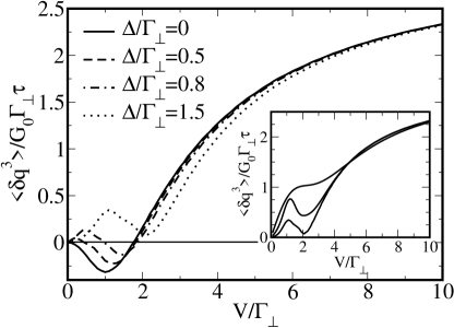
Figure 1: Zero temperature voltage dependence of the third cumulant for different magnetic field values and $\Gamma_{\pm}/\Gamma_{\perp}=0.1$. Inset: temperature evolution of the curve for $\Delta/\Gamma_{\perp}=1.5$ for $T/\Gamma_{\perp}=0$, $0.2$ and $1.5$ (from bottom to top).

III.6.2 Corrections around the Toulouse point

Thus far we dealt with a system which finds itself at one special point in the parameter space, when $v_{1}=0$ and $J_{z-}=0$. While the latter requirement is reasonable for realistic systems, the former is quite artificial. It has been shown by means of RG transformation procedure that at least in equilibrium the operators, describing deviations from the Toulouse point are irrelevant in the RG sense and do not influence the physics in the low energy sector strongly. There is, however, no a priori reason why that should hold in a non-equilibrium situation. Therefore the full analysis of the FCS must incorporate the investigation of the statistics beyond the Toulouse restrictions. We first concentrate on the situation of finite $v_{1}$. As was pointed out above, an analytic solution in this situation is not possible. The only option to progress is perturbation theory in $v_{1}$.

To access the generating function we still can use the fundamental relation (78). As we have the complete knowledge of all GFs with respect to $H^{\prime}$, see (68), the simplest thing we can do is to calculate perturbative corrections to $D_{bb}$ in the second order in $v_{1}$. They are given by

$$\hat{\bar{D}}_{bb}=\hat{D}_{bb}+v_{1}^{2}\hat{D}_{bb}\,\hat{\Sigma}_{b}\,\hat{D}_{bb}=\hat{D}_{bb}+\delta\hat{D}_{bb}\,.$$

The correction to the adiabatic potential is then given by

$$\delta\left(\frac{\partial\cal U}{\partial\lambda_{-}}\right)=i\frac{\Gamma_{\perp}}{2}\int\,\frac{d\omega}{2\pi}\,\left\{\delta D_{bb}^{--}(n_{R}-n_{L})+\delta D_{bb}^{-+}\left[e^{i\bar{\lambda}/2}(1-n_{R})-e^{-i\bar{\lambda}/2}(1-n_{L})\right]\right\}\,.$$

The self-energy matrix components are defined as

$$\Sigma^{ij}_{b}(\omega)=\int\frac{d\epsilon_{1}}{2\pi}\,D^{ij}_{aa}(\omega-\epsilon_{1})\,\int\frac{d\epsilon_{2}}{2\pi}\,G^{ij}_{s}(\epsilon_{2})G^{ji}_{s}(\epsilon_{1}+\epsilon_{2})\,,$$

where $G_{s}(t,t^{\prime})=-i\langle T_{C}\psi_{s}(t)\psi^{\dagger}_{s}(t^{\prime})\rangle_{\lambda}$ is the GF of the spin sector fermion which is free. Therefore at $T=0$ it is easily found to be

$$G_{s}(\omega)=\left[\begin{array}[]{cc}-\frac{i}{2}\mbox{sgn}(\omega)&i\Theta(-\omega)\\ -i\Theta(\omega)&-\frac{i}{2}\mbox{sgn}(\omega)\\ \end{array}\right]\,,$$ (98)

In the $\Delta=0$ and $\Gamma_{+}=0$ case only $D_{aa}^{--(++)}=\pm d_{0}=\pm 1/\omega$ are non-zero, so that only $\Sigma_{b}^{--}$ needs to be calculated, resulting in

$$\Sigma_{b}^{--}(\omega)=-\Sigma_{b}^{++}(\omega)=(2\pi)^{-2}\omega\left(\ln|\omega|-1\right)\,.$$

It is an odd function of $\omega$ and vanishes in the infrared limit as expected from RG arguments since it is generated by an irrelevant operator. The corrections to the impurity GFs are then

$$\delta D_{bb}^{--}=v_{1}^{2}\,\Sigma_{b}^{--}\left(D_{bb}^{--}D_{bb}^{--}-D_{bb}^{-+}D_{bb}^{+-}\right)\,\,\,,\,\,\,\delta D_{bb}^{-+}=v_{1}^{2}\,\Sigma_{b}^{--}D_{bb}^{-+}\left(D_{bb}^{--}-D_{bb}^{++}\right)\,.$$

Furthermore,

$$D_{bb}^{--}D_{bb}^{--}-D_{bb}^{-+}D_{bb}^{+-} = \mbox{Det}^{-1}\,(\hat{d}_{0}^{-1}-\hat{\Sigma}_{K})+\frac{2\omega\left\{\omega+i\left[\Gamma_{-}(2n_{F}-1)+\Gamma_{\perp}(n_{R}+n_{L}-1)\right]\right\}}{\mbox{Det}^{2}\,(\hat{d}_{0}^{-1}-\hat{\Sigma}_{K})}\,,$$

and is an even function of $\omega$. After multiplication with the self-energy, which is an odd function, and after an integration over all frequencies we immediately see, that the off–Toulouse correction to the first contribution in (78) is identically zero:

$$\ D_{bb}^{-+}\left(D_{bb}^{--}-D_{bb}^{++}\right) = -2i\omega\frac{\Gamma_{-}\,2n_{F}+\Gamma_{\perp}(e^{i\bar{\lambda}/2}n_{L}+e^{-i\bar{\lambda}/2}n_{R})}{\mbox{Det}^{2}\,(\hat{d}_{0}^{-1}-\hat{\Sigma}_{K})}\,.$$

Therefore for the correction to the derivative of the adiabatic potential we obtain

$$\delta\left(\frac{\partial{\cal U}}{\partial\lambda_{-}}\right)=-v_{1}^{2}\Gamma_{\perp}\int\frac{d\omega}{2\pi}\,\frac{\Sigma_{b}^{--}}{\mbox{Det}^{2}\,(\hat{d}_{0}^{-1}-\hat{\Sigma}_{K})}\omega\left\{2\Gamma_{-}n_{F}[e^{i\bar{\lambda}/2}(1-n_{R})-e^{-i\bar{\lambda}/2}(1-n_{L})]\right.$$

$$\left.+\Gamma_{\perp}[e^{i\bar{\lambda}}n_{L}(1-n_{R})-e^{-i\bar{\lambda}}n_{R}(1-n_{L})]\right\}\,,$$

Comparing this result with (89) we conclude that the effect of $v_{1}$ is the correction to the transmission coefficients $\bar{T}_{i}=T_{i}+\delta T_{i}$ with

$$\delta T_{i}(\omega)=\left(\frac{v_{1}}{2\pi}\right)^{2}\frac{\omega^{2}}{\omega^{2}+(\Gamma_{-}+\Gamma_{\perp})^{2}}\left(\ln|\omega|-1\right)T_{i}(\omega)\,,$$

since schematically the structure of the correction is

$$\frac{2T_{2}e^{2i\lambda}+T_{1}e^{i\lambda}}{1+T_{2}(e^{2i\lambda}-1)+T_{1}(e^{i\lambda}-1)}+\delta\frac{2T_{2}e^{2i\lambda}+T_{1}e^{i\lambda}}{[1+T_{2}(e^{2i\lambda}-1)+T_{1}(e^{i\lambda}-1)]^{2}}\;,$$

which can be seen as the lowest order expansion of

$$\frac{2T_{2}(1+\delta)e^{2i\lambda}+T_{1}(1+\delta)e^{i\lambda}}{1+T_{2}(1+\delta)(e^{2i\lambda}-1)+T_{1}(1+\delta)(e^{i\lambda}-1)}\,.$$

This correction vanishes for $\omega\rightarrow 0$, hence the trivialisation (94) still holds for the transmission coefficients away from the Toulouse point.

It is not clear whether this picture is valid for $\Gamma_{+}$, $\Delta\neq 0$. As in this situation the magnetic field couples the $a$ and $b$ Majorana fields, the $D_{aa}$ correlation functions have to be calculated from the Dyson equation with respect to the self-energy $\Sigma_{a}^{ij}=(ij)\left[\Delta^{2}D_{bb}^{ij}(\Delta=0)+\Gamma_{+}g^{(0)ij}_{\eta\eta}\right]$. As our ultimate goal is the behaviour of the generating function in the limiting case of small $V$, we set $V=0$. We return to the finite $V$ situation at the end of this Section. The resulting $\Sigma_{b}$ can be best given in terms of the retarded component $\Sigma_{b}^{R}$,

$$\Sigma_{b}^{--(++)} = \pm\,\mbox{Re}\Sigma_{b}^{R}-i\,(2n_{F}-1)\,\mbox{Im}\Sigma_{b}^{R}\,,$$

$$\Sigma_{b}^{-+} = i\,2n_{F}\,\mbox{Im}\Sigma_{b}^{R}\,,$$ (99)

$$\Sigma_{b}^{+-} = -i\,2(1-n_{F})\,\mbox{Im}\Sigma_{b}^{R}\,,$$

with

$$\Sigma_{b}^{R} = \frac{i}{(2\pi)^{2}}\frac{1}{\sqrt{b^{2}-4d}}\sum_{j=1,2}\,[\Omega^{2}_{j}+\Delta^{2}-(\Gamma_{-}+\Gamma_{\perp})^{2}]\left\{(\Omega_{j}-i\omega)\left[\ln(\Omega_{j}-i\omega)-1\right]-\Omega_{j}(\ln\Omega_{j}-1)\right\}\,,$$

where $b=(\Gamma_{-}+\Gamma_{\perp})^{2}+\Gamma_{+}^{2}-2\Delta^{2}$, $d=[\Delta^{2}+\Gamma_{+}(\Gamma_{-}+\Gamma_{\perp})]^{2}$, and $\Omega^{2}_{1,2}=(b\pm\sqrt{b^{2}-4d})/2$. The expansion for small energies is different from that at $\Delta=0$,

$$\mbox{Re}\Sigma^{R} \approx -\frac{\omega}{(2\pi)^{2}\sqrt{b^{2}-4d}}\sum_{j=1,2}\,[\Omega^{2}_{j}+\Delta^{2}-(\Gamma_{-}+\Gamma_{\perp})^{2}]\ln\Omega_{j}$$

$$\mbox{Im}\Sigma^{R} \approx -i\frac{\omega^{2}}{(2\pi)^{2}2\sqrt{b^{2}-4d}}\sum_{j=1,2}\,[\Omega^{2}_{j}+\Delta^{2}-(\Gamma_{-}+\Gamma_{\perp})^{2}]\frac{\ln\Omega_{j}}{\Omega_{j}}\,.$$

The correction to the time ordered part is,

$$\delta D_{bb}^{--} = v_{1}^{2}\,\left(D_{bb}^{--}\Sigma_{b}^{--}D_{bb}^{--}+D_{bb}^{-+}\Sigma_{b}^{++}D_{bb}^{+-}+D_{bb}^{-+}\Sigma_{b}^{+-}D_{bb}^{--}+D_{bb}^{--}\Sigma_{b}^{-+}D_{bb}^{+-}\right)\,$$

$$= v_{1}^{2}\left(D_{bb}^{--}D_{bb}^{--}-D_{bb}^{-+}D_{bb}^{+-}\right)\mbox{Re}\Sigma_{b}^{R}+iv_{1}^{2}\,\mbox{Im}\Sigma_{b}^{R}\,{\cal F}_{1}(\omega)\;,$$

with

$${\cal F}_{1}(\omega)=-(2n_{F}-1)\left(D_{bb}^{--}D_{bb}^{--}+D_{bb}^{-+}D_{bb}^{+-}\right)-2(1-n_{F})D_{bb}^{--}D_{bb}^{-+}+2n_{F}D_{bb}^{--}D_{bb}^{+-}\,.$$

This function is an odd function of $\omega$ while $D_{bb}^{--}D_{bb}^{--}-D_{bb}^{-+}D_{bb}^{+-}$ is even. Taking into account the symmetry properties of the self-energy we conclude that the whole contribution to the generating function stemming from $\delta D_{bb}^{--}$ vanishes. The other component can be written down in the similar way,

$$\delta D_{bb}^{-+} = v_{1}^{2}\,\left(D_{bb}^{--}\Sigma_{b}^{--}D_{bb}^{-+}+D_{bb}^{-+}\Sigma_{b}^{++}D_{bb}^{++}+D_{bb}^{-+}\Sigma_{b}^{+-}D_{bb}^{-+}+D_{bb}^{--}\Sigma_{b}^{-+}D_{bb}^{++}\right)$$

$$= v_{1}^{2}D_{bb}^{-+}(D_{bb}^{--}-D_{bb}^{++})\mbox{Re}\Sigma_{b}^{R}+\,iv_{1}^{2}\,\mbox{Im}\Sigma_{b}^{R}{\cal F}_{2}(\omega)\,,$$

where we have introduced

$${\cal F}_{2}(\omega) = (1-2n_{F})D_{bb}^{-+}(D_{bb}^{--}+D_{bb}^{++})+2(1-n_{F})D_{bb}^{-+}D_{bb}^{-+}-2n_{F}D_{bb}^{--}D_{bb}^{++}\,.$$ (100)

The analysis of the contribution arising from Re$\Sigma_{b}^{R}$ can be done in the same way as before as it has exactly the same structure. The substitution (110) still can be applied and one immediately recognises that it only leads to the renormalisation of the transmission coefficients,

$$\delta T_{i}(\omega)=v_{1}^{2}\mbox{Re}\Sigma_{b}^{R}\frac{\omega(\omega^{2}+\Gamma_{+}^{2}-\Delta^{2})}{\left[\omega^{2}-\Delta^{2}-\Gamma_{+}(\Gamma_{\perp}+\Gamma_{-})\right]^{2}+\omega^{2}(\Gamma_{-}+\Gamma_{+}+\Gamma_{\perp})^{2}}T_{i}(\omega)\,.$$ (101)

Re$\Sigma_{b}^{R}$ is itself linear in $\omega$ in the low energy sector, that is why the corrections to the transmission coefficients (101) vanish at low energies. Now we turn to the contribution of Im$\Sigma_{b}^{R}$. The first term in (100) can be shown to produce renormalisation of the transmission coefficient similar to (101),

$$\delta T_{i}(\omega)=v_{1}^{2}\mbox{Im}\Sigma_{b}^{R}\frac{\Gamma_{-}\left[\Gamma_{-}(\omega^{2}+\Gamma_{+}^{2})+\Delta^{2}\Gamma_{+}\right]}{\left[\omega^{2}-\Delta^{2}-\Gamma_{+}(\Gamma_{\perp}+\Gamma_{-})\right]^{2}+\omega^{2}(\Gamma_{-}+\Gamma_{+}+\Gamma_{\perp})^{2}}T_{i}(\omega)\,.$$

Although the two remaining terms of (100) cannot be reduced to renormalisation of the transmission coefficients in a simple way, their contribution to the derivative of the adiabatic potential can be evaluated directly,

$$\delta_{I}\left(\frac{\partial{\cal U}}{\partial\lambda_{-}}\right)=v^{2}\frac{\Gamma_{\perp}}{2}\int_{0}^{V}\,\frac{d\omega}{2\pi}\,\mbox{Im}\Sigma_{b}^{R}e^{i\bar{\lambda}/2}\mbox{Det}^{-2}\,(\hat{d}_{0}^{-1}-\hat{\Sigma}_{K})\left[\left(\omega-\frac{\Delta^{2}\omega}{\omega^{2}+\Gamma_{+}^{2}}\right)^{2}+\left(\Gamma_{-}+\frac{\Delta^{2}\Gamma_{+}}{\omega^{2}+\Gamma_{+}^{2}}\right)^{2}+\Gamma_{\perp}^{2}e^{i\bar{\lambda}}\right]\,.$$

Taking into account that the leading behaviour of the imaginary part of the self-energy is $\sim\omega^{2}$ for small energies one immediately verifies, that the above correction is cubic in the applied voltage and therefore leads to qualitatively the same picture as the renormalisation of the transmission coefficients. For that particular evaluation we used the equilibrium self-energy $\hat{\Sigma}_{b}$. Nevertheless, after a lengthy but straightforward calculation, we find that the same conclusion is still valid for the proper non-equilibrium one as the corresponding corrections to $\hat{\Sigma}_{b}$ is of exactly the same order in $V$ and $\omega$. Thus at least in the low energy sector the predictions of Sec. III.6.1 remain valid beyond the Toulouse point.

III.6.3 Resonant level problem in Luttinger liquids

We now briefly turn to the $g=1/2$ RL set–up. This set–up has caused much interest recently, see Ref. ourPRL and references therein. The Hamiltonian now is

$$H=H_{0}+(\gamma_{L}\,\psi_{L}d^{\dagger}+\gamma_{R}\,d\psi_{R}^{\dagger}+{\rm H.c})+\Delta d^{\dagger}d+H_{C}\;,$$

where $H_{0}$ stands for two biased Luttinger liquids (LLs), $d$ is the electron operator on the dot, $\gamma_{R(L)}$ are the tunnelling amplitudes to $R(L)$ electrode and $H_{C}$ is an electrostatic interaction (see also ourPRL ),

$$H_{C}=\lambda_{C}d^{\dagger}d\,\sum_{i}\,\psi_{i}^{\dagger}(0)\psi_{i}(0)\,.$$

The contacting electrodes are supposed to be one-dimensional half-infinite electron systems. We model them by chiral fermions living in an infinite system: the negative half-axis then describes the particles moving towards the boundary, while the positive half-axis carries electrons moving away from the end of the system. In the bosonic representation $H_{0}[\psi_{i}]$ are diagonal even in presence of interactions (for a recent review see e. g. book ; we set the renormalised Fermi velocity $v=v_{F}/g=1$, the bare velocity being $v_{F}$):

$$H_{0}[\psi_{i}]=(4\pi)^{-1}\int\,dx\,[\partial_{x}\phi_{i}(x)]^{2}.$$

Here the phase fields $\phi_{i}(x)$ describe the slow varying spatial component of the electron density (plasmons),

$$\psi^{\dagger}_{i}(x)\psi_{i}(x)=\partial_{x}\phi_{i}(x)/2\pi\sqrt{g}\,.$$

The electron field operator at the boundary is given by ,

$$\psi_{i}(0)=e^{i\phi_{i}(0)/\sqrt{g}}/\sqrt{2\pi a_{0}}\,,$$

where $a_{0}$ is the lattice constant of the underlying lattice model. Here $g$ is the conventional LL parameter (coupling constant) connected to the bare interaction strength $U$ via $g=(1+U/\pi v_{F})^{-1/2}$ book ; kanefisher . In the chiral formulation the bias voltage amounts to a difference in the densities of the incoming particles in both channels far away from the constriction eggergrabert ; grabert . The current is then proportional to the difference between the densities of incoming and outgoing particles within each channel.

Construction of the operator (2) is unproblematic and leads to

$$T_{\lambda}=\gamma_{L}(d^{\dagger}\psi_{L}e^{i\lambda/4}+\psi_{L}^{\dagger}de^{-i\lambda/4}) + \gamma_{R}(d^{\dagger}\psi_{R}e^{-i\lambda/4}+\psi_{R}^{\dagger}de^{i\lambda/4})\,,$$

where, contrary to the Anderson impurity calculation, we choose to build in the counting field in a symmetric manner for the reasons which will become clear later. After the Emery–Kivelson rotation, refermionization to new fermions $\psi$ and after the introduction of the Majorana components as in (67) EK ; ourPRB we find

$$T_{\lambda} = \left[e^{i\lambda/4}(\gamma_{L}d^{\dagger}\psi+\gamma_{R}\psi d)+e^{-i\lambda/4}(\gamma_{L}d^{\dagger}\psi^{\dagger}+\gamma_{R}\psi^{\dagger}d)\right]$$ (102)

$$= -i\gamma_{+}\,b\left[\cos(\lambda/4)\xi-\sin(\lambda/4)\eta\right]+i\gamma_{-}\,a\left[\sin(\lambda/4)\xi-\cos(\lambda/4)\eta\right]\;.$$

where $\gamma_{\pm}=\gamma_{L}\pm\gamma_{R}$. In case of the symmetric coupling $\gamma_{-}=0$ the corresponding $T_{\lambda}$ has exactly the same shape as (69). In fact we find the same set of equations as for the Kondo dot, Eq. (68) and Eq. (69), but with $\lambda\to\lambda/2$ and $J_{\perp}=\gamma_{+}$, $J_{\pm}=0$. Consequently, the FCS is given by a modification of the Levitov–Lesovik formula (II.2):

$$\chi_{1/2}(\lambda)=\chi_{0}(\lambda;2V;\{T_{\Delta}(\omega)\})\;,$$ (103)

with the effective transmission coefficient $T_{\Delta}(\omega)=4\gamma^{4}\omega^{2}/[4\gamma^{4}\omega^{2}+(\omega^{2}-\Delta^{2})^{2}]$ of the RL set-up in the symmetric case ourPRL . All the cumulants are thus obtainable from those of the non-interacting statistics Eq. (II.2).

The $\Delta=0$ RL set–up is equivalent to the model of direct tunnelling between two $g=2$ LLs ourPRB . The latter model is connected by the strong to weak coupling ($1/g\to g$) duality argument to the $g=1/2$ Kane and Fisher model kanefisher ; saleurduality , which is, in turn, equivalent to the CB set–up studied in AM ; KT (for a more general case of arbitrary interaction strength see also weisssaleur ; safi ). Therefore their FCS must be related to our Eq. (103) at $\Delta=0$ by means of the transformation: $T_{0}\to 1-T_{0}$ and $V\to V/2$. Indeed after some algebraic manipulation with Eq. (12) of KT , for details see Appendix C, we find that the FCS for the CB set–up can be re–written as:

$$\chi_{CB}(\lambda)=\chi_{0}(-\lambda;V;\{1-T_{0}(\omega)\})\;.$$

For the asymmetric coupling $\gamma_{-}\neq 0$ the problem cannot be mapped onto the Kondo dot any more. The corresponding calculation is nevertheless straightforward and is presented in Appendix D. There is no fundamental difference in the result up to the more involved transmission coefficient, which has already been derived for the case of the non-linear $I-V$ in ourPRL .

IV Conclusions

To conclude, we present a detailed study of the charge transfer statistics through the Anderson impurity model. We find an expression for the exact generating function in terms of the impurity self–energy calculated in the presence of the measuring field $\lambda$: Eq. (III.3). Based on this formula we conclude that $T=0$ linear response statistics is universal and binomial for the AIM and similar models: we call this fact binomial theorem. The only effect of correlations is to define an effective transmission coefficient. For the symmetric AIM, for example, there is a perfect transmission and no fluctuations of the current at all in this case.

In the search for non-trivial interaction effects one has, therefore, to go to higher values of $T$ and $V$. To this end we have calculated the exact FCS distribution function in the Toulouse limit (Kondo regime): it is given by Eq. (III.6.1). This formula uncovers rather profound, if model dependent, consequences of correlations: there are two distinct tunnelling processes ($T_{1}$ and $T_{2}$), that of single electrons and electron pairs with opposite spin. The latter process is, in fact, dominant in zero field. The structure of higher moments is also determined by these two processes as discussed in detail in the main text. At $T=0$ linear response all this rich physics is masked by Eq. (III.6.1) collapsing to the universal binomial distribution. We checked this universality by extensively studying corrections to the distribution function due to departures from the Toulouse limit.

We close by outlining some possible directions for future developments. Formula (III.3) could be used to develop Fermi liquid theory for the noise and possibly higher moments. Perhaps more importantly, the ideas of this paper could be applied to models with many conduction channels, where one would expect some equivalent of the binomial theorem to hold, as seems to be compatible with recent experiments bomze .

Appendix A

The calculation of the impurity GF in finite magnetic field $\Delta$ and $J_{+}\neq 0$ is accomplished again by inversion of $\hat{d}_{0}^{-1}-\hat{\Sigma}_{\Delta}$ with

$$\hat{\Sigma}_{\Delta}=\left[\begin{array}[]{cc}\Delta^{2}D_{aa}^{--}+\Sigma^{--}_{K}&-\Delta^{2}D_{aa}^{-+}+\Sigma^{-+}_{K}\\ -\Delta^{2}D_{aa}^{+-}+\Sigma^{+-}_{K}&\Delta^{2}D_{aa}^{++}+\Sigma^{++}_{K}\end{array}\right]\;,$$ (106)

where $\hat{\Sigma}_{K}$ is given in (81). $\hat{D}_{aa}$ has to be evaluated with respect to the Hamiltonian

$$H_{+}=H_{0}[\eta_{f}]-iJ_{+}\,a\,\eta_{f}\,.$$

A relatively simple calculation yields

$$D_{aa}(\omega)=\frac{1}{\omega^{2}+\Gamma_{+}^{2}}\left[\begin{array}[]{cc}\omega+i\Gamma_{+}(2n_{F}-1)&i2\Gamma_{+}n_{F}\\ -i2\Gamma_{-}(1-n_{F})&-\omega+i\Gamma_{+}(2n_{F}-1)\\ \end{array}\right]\,.$$ (109)

From now on the calculation can be performed in exactly the same way as before. However, writing down explicitly the expression for $\hat{\Sigma}_{\Delta}$ one observes, that it can be constructed from the corresponding $\hat{\Sigma}_{K}$ via trivial substitution

$$\omega\rightarrow\omega-\frac{\Delta^{2}\omega}{\omega^{2}+\Gamma_{+}^{2}}\,\,\,,\,\,\,\Gamma_{-}\rightarrow\Gamma_{-}+\frac{\Delta^{2}\Gamma_{+}}{\omega^{2}+\Gamma_{+}^{2}}\,.$$ (110)

This can be used to obtain the transmission coefficients (III.6.1) from the ones given by (91).

Appendix B

For systems with known scattering matrix $s_{\alpha\beta,mn}$ between terminals $\alpha,\beta$ and channels $m$ and $n$, there is a ready formula for the FCS generating function, derived in levitovlesovik ,

$$\ln\chi(\lambda)=\frac{\cal T}{2\pi}\int\,d\omega\,\ln\mbox{Det}\,\left[1+\hat{f}(\omega)\,\left(\hat{s}^{\dagger}\,\widetilde{s}\,-1\right)\right]\,,$$ (111)

where $\widetilde{s}_{\alpha\beta,mn}=e^{i(\lambda_{\alpha}-\lambda_{\beta})}s_{\alpha\beta,mn}$, $\lambda_{\alpha,\beta}$ being the fields counting the particles in the respective terminals. $\hat{f}(\omega)=\delta_{mn}\,\delta_{\alpha\beta}\,f_{\alpha}(\omega)$ is diagonal in both channel ($m,n$) and terminal ($\alpha,\beta$) indices and describes the energy distribution function in the respective terminal. In the simplest situation, when $\Delta=0$ and $J_{+}=0$, we have four terminals with one channel in each of them. The scattering part of the Hamiltonian is $H_{I}=J_{\perp}(\psi^{\dagger}-\psi)\,b+J_{-}(\psi_{s}^{\dagger}-\psi_{s})\,b$, see (66)(for simplicity we ignore the unimportant numerical prefactors). The equations of motion (EoMs) for the participating operators read

$$i\partial_{t}\psi_{s} = -i\partial_{x}\psi_{s}+J_{-}b\delta(x)\,,$$

$$i\partial_{t}\psi = -i\partial_{x}\psi+J_{\perp}b\delta(x)\,,$$

$$i\partial_{t}b = J_{\perp}(\psi^{\dagger}-\psi)+J_{-}(\psi_{s}^{\dagger}-\psi_{s})\,.$$

Integrating the first equation over time and then around the point $x=0$ we obtain

$$i\left[\psi_{s}(0^{+})-\psi_{s}(0^{-})\right]=J_{-}b\,.$$

Acting with $i\partial_{t}$ from the left and using the EoM for the $b$ Majorana one obtains,

$$-\partial_{t}\left[\psi_{s}(0^{+})-\psi_{s}(0^{-})\right] = J_{-}J_{\perp}(\psi^{\dagger}-\psi)+J_{-}^{2}(\psi_{s}^{\dagger}-\psi_{s})\,,$$

$$-\partial_{t}\left[\psi(0^{+})-\psi(0^{-})\right] = J_{-}J_{\perp}(\psi_{s}^{\dagger}-\psi_{s})+J_{\perp}^{2}(\psi^{\dagger}-\psi)\,,$$

where the last equation is obtained by symmetry. Now we employ the plain wave decomposition similar to that used in wen ; eggergrabert ; ourPRL ,

$$\psi(x)=\int\,\frac{dk}{2\pi}\,e^{ik(x-t)}\,\left\{\begin{array}[]{cc}a_{k}&\mbox{for}\,x<0\\ b_{k}&\mbox{for}\,x>0\end{array}\right.\,\,\,,\,\,\,\psi_{s}(x)=\int\,\frac{dk}{2\pi}\,e^{ik(x-t)}\,\left\{\begin{array}[]{cc}c_{k}&\mbox{for}\,x<0\\ d_{k}&\mbox{for}\,x>0\end{array}\right.\,.$$ (116)

Since the dispersion relation of both fermion species is trivial, $\omega=k$, we can use $\omega$ both for momentum and energy. Employing the regularisation scheme $\psi_{i}=[\psi(0^{+})+\psi(0^{-})]/2$ we obtain

$$-i\omega\left(d_{\omega}-c_{\omega}\right) = \frac{J_{\perp}J_{-}}{2}\left(a_{-\omega}^{\dagger}+b_{-\omega}^{\dagger}-a_{\omega}-b_{\omega}\right)+\frac{J_{-}^{2}}{2}\left(c_{-\omega}^{\dagger}+d_{-\omega}^{\dagger}-c_{\omega}-d_{\omega}\right)\,,$$

$$-i\omega\left(b_{\omega}-a_{\omega}\right) = \frac{J_{\perp}J_{-}}{2}\left(c_{-\omega}^{\dagger}+d_{-\omega}^{\dagger}-c_{\omega}-d_{\omega}\right)+\frac{J_{\perp}^{2}}{2}\left(a_{-\omega}^{\dagger}+b_{-\omega}^{\dagger}-a_{\omega}-b_{\omega}\right)\,.$$

Comparing these relations with their adjunct at $-\omega$ we identify that

$$b_{-\omega}^{\dagger} = a_{-\omega}^{\dagger}-b_{\omega}+a_{\omega}\,,$$

$$d_{-\omega}^{\dagger} = c_{-\omega}^{\dagger}-d_{\omega}+c_{\omega}\,,$$

and that $b_{\omega}-a_{\omega}=(d_{\omega}-c_{\omega})\,J_{\perp}/J_{-}$. Using these expressions we can find both $b_{\omega}$ and $d_{\omega}$ as functions of $a_{\omega}$ and $c_{\omega}$, e. g.

$$b_{\omega}=\frac{1}{\omega+i(\Gamma_{\perp}+\Gamma_{-})}\left[(\omega+i\Gamma_{-})\,a_{\omega}+i\Gamma_{\perp}\,a_{-\omega}^{\dagger}-iJ_{\perp}J_{-}\,c_{\omega}+iJ_{\perp}J_{-}\,c_{-\omega}^{\dagger}\right]\,.$$

That leads to the following scattering matrix,

$$\left(\begin{array}[]{c}b_{\omega}\ b_{-\omega}^{\dagger}\\ d_{\omega}\\ d_{-\omega}^{\dagger}\end{array}\right)=s\,\left(\begin{array}[]{c}a_{\omega}\\ a_{-\omega}^{\dagger}\\ c_{\omega}\\ c_{-\omega}^{\dagger}\end{array}\right)=\frac{1}{\omega+i(\Gamma_{\perp}+\Gamma_{-})}\left(\begin{array}[]{cccc}\omega+i\Gamma_{-}&i\Gamma_{\perp}&-iJ_{\perp}J_{-}&iJ_{\perp}J_{-}\\ i\Gamma_{\perp}&\omega+i\Gamma_{-}&iJ_{\perp}J_{-}&-iJ_{\perp}J_{-}\\ -iJ_{\perp}J_{-}&iJ_{\perp}J_{-}&\omega+i\Gamma_{\perp}&i\Gamma_{-}\\ iJ_{\perp}J_{-}&-iJ_{\perp}J_{-}&i\Gamma_{-}&\omega+i\Gamma_{\perp}\end{array}\right)\,\left(\begin{array}[]{c}a_{\omega}\\ a_{-\omega}^{\dagger}\\ c_{\omega}\\ c_{-\omega}^{\dagger}\end{array}\right)\,.$$ (132)

The actual charge transport through the system is conveyed by the charge flavour channel, e. g. by scattering of $\psi$ fermions across the constriction. The physical picture is similar to that discussed in ourPRL : the incoming particles – chiral fermions in terminal $1$, which are described by $a_{k}$ operators and which have chemical potential $\mu_{1}=V$ – are transferred into all other terminals $2$-$4$ ($b_{k}$, $c_{k}$ and $d_{k}$ operators), which are unbiased $\mu_{2,3,4}=0$, that is why we have to set $\hat{f}=\mbox{diag}(n_{L},n_{F},n_{F},n_{F})$. Then $\lambda_{1}=\lambda$ counts particles which leave channel $1$. However, the very same fermion reappears in the channel $2$. Since $1$ and $2$ are physically one lead we have $\lambda_{2}=-\lambda$. We are not interested in change of particle numbers in the other channels, that is why $\lambda_{3,4}=0$ . Therefore the matrix $\widetilde{s}$ is given by

$$\widetilde{s}=\frac{1}{\omega+i(\Gamma_{\perp}+\Gamma_{-})}\left(\begin{array}[]{cccc}\omega+i\Gamma_{-}&i\Gamma_{\perp}\,e^{-i2\lambda}&-iJ_{\perp}J_{-}\,e^{-i\lambda}&iJ_{\perp}J_{-}\,e^{-i\lambda}\\ i\Gamma_{\perp}\,e^{i2\lambda}&\omega+i\Gamma_{-}&iJ_{\perp}J_{-}e^{i\lambda}&-iJ_{\perp}J_{-}e^{i\lambda}\\ -iJ_{\perp}J_{-}\,e^{i\lambda}&iJ_{\perp}J_{-}e^{-i\lambda}&\omega+i\Gamma_{\perp}&i\Gamma_{-}\\ iJ_{\perp}J_{-}\,e^{i\lambda}&-iJ_{\perp}J_{-}e^{-i\lambda}&i\Gamma_{-}&\omega+i\Gamma_{\perp}\end{array}\right)\,.$$ (137)

Plugging these relations into (111), folding the integration over energy to the domain $[0,\infty)$ and using the properties $n_{F}(-\omega)=1-n_{F}(\omega)$ and $n_{L}(-\omega)=1-n_{R}(\omega)$ immediately leads then to the result (III.6.1).

Appendix C

Here we establish the relation between our findings and the result of Kindermann and Trauzettel (KT) calculation KT . Let us consider Eq. (12) of Ref. KT ,

$$\ln\chi_{KT}(\lambda)=\frac{\cal T}{4\pi}(-iV\lambda-T^{2}\lambda^{2})+{\cal T}\int\limits_{0}^{\infty}\frac{d\omega}{2\pi}\ln\left\{1+T_{0}(\omega)[f^{+}(1-f^{-})(e^{i\lambda}-1)+f^{-}(1-f^{+})(e^{-i\lambda}-1)]\right\}\;,$$

The $f$-functions are given by

$$f^{\pm}=\frac{n_{L/R}}{(1-n_{L/R})e^{\pm i\lambda}+n_{L/R}}\;,$$

where $n_{R,L}(\omega)=n_{F}(\omega\pm V/2)$. Obviously

$$1-f^{\pm}=\frac{(1-n_{L/R})e^{\pm i\lambda}}{(1-n_{L/R})e^{\pm i\lambda}+n_{L/R}}\;,$$

Taking into account that $T_{0}(\omega)=4\gamma^{4}/(\omega^{2}+4\gamma^{2})$, the identification with the KT’s impurity strength is $2\gamma=T_{B}$. In order to proceed we define the object

$$\ln\chi_{KT}(\lambda;\alpha)=\frac{\cal T}{4\pi}(-iV\lambda-T^{2}\lambda^{2})+{\cal T}\int\limits_{0}^{\infty}\frac{d\omega}{2\pi}\ln\left\{1+\alpha T_{0}(\omega)[f^{+}(1-f^{-})(e^{i\lambda}-1)+f^{-}(1-f^{+})(e^{-i\lambda}-1)]\right\}\;,$$ (138)

where $\alpha$ is a parameter. The derivative of (138) with respect to this parameter

$$\frac{\partial\ln\chi_{KT}(\lambda;\alpha)}{\partial\alpha}={\cal T}\int\limits_{0}^{\infty}\frac{d\omega}{2\pi}\frac{T_{0}(\omega)[f^{+}(1-f^{-})(e^{i\lambda}-1)+f^{-}(1-f^{+})(e^{-i\lambda}-1)]}{1+\alpha T_{0}(\omega)[f^{+}(1-f^{-})(e^{i\lambda}-1)+f^{-}(1-f^{+})(e^{-i\lambda}-1)]}\;.$$

Substituting explicit expressions for the $f$–functions into the long fraction gives

$$-\frac{T_{0}(\omega)[n_{L}(1-n_{R})(e^{-i\lambda}-1)+n_{R}(1-n_{L})(e^{i\lambda}-1)]}{[(1-n_{L})e^{i\lambda}+n_{L}][(1-n_{L})e^{-i\lambda}+n_{R}]-\alpha T_{0}(\omega)[n_{L}(1-n_{R})(e^{-i\lambda}-1)+n_{R}(1-n_{L})(e^{i\lambda}-1)]}\;.$$

After simple algebra this simplifies as

$$-\frac{T_{0}(\omega)[n_{L}(1-n_{R})(e^{-i\lambda}-1)+n_{R}(1-n_{L})(e^{i\lambda}-1)]}{1+[1-\alpha T_{0}(\omega)][n_{L}(1-n_{R})(e^{-i\lambda}-1)+n_{R}(1-n_{L})(e^{i\lambda}-1)]}\;.$$

Integrating with respect to $\alpha$ therefore results in

$$\ln\chi_{KT}(\lambda;\alpha)={\cal T}\int\limits_{0}^{\infty}\frac{d\omega}{2\pi}\ln\left\{1+[1-\alpha T_{0}(\omega)][n_{L}(1-n_{R})(e^{-i\lambda}-1)+n_{R}(1-n_{L})(e^{i\lambda}-1)]\right\}+C\;.$$

To fix the constant $C$, evaluate the above integral at $\alpha=0$, see also lll

$${\cal T}\int\limits_{0}^{\infty}\frac{d\omega}{2\pi}\ln[1+n_{L}(1-n_{R})(e^{-i\lambda}-1)+n_{R}(1-n_{L})(e^{i\lambda}-1)]=\frac{\cal T}{4\pi}(-iV\lambda-T^{2}\lambda^{2})\,,$$

so that $C=0$. The following identity is therefore established (put $\alpha=1$):

$$\ln\chi_{KT}(\lambda)=\tau\int\limits_{0}^{\infty}\frac{d\omega}{2\pi}\ln\left\{1+[1-T_{0}(\omega)][n_{L}(1-n_{R})(e^{-i\lambda}-1)+n_{R}(1-n_{L})(e^{i\lambda}-1)]\right\}$$ (139)

The two equations (Appendix C) and (139) define the same function, which means that the KT statistics, like the $g=1/2$ statistics, is reducible to the generic Levitov-Lesovik formula, its relation to the non–interacting statistics Eq. (II.2) being

$$\chi_{KT}(\lambda)=\chi_{0}(-\lambda;V;\{1-T_{0}(\omega)\})\;.$$

Finally the explicit relation between the KT statistics and our $g=1/2$ result is

$$\chi_{KT}(\lambda;V;\{T_{0}(\omega)\})=\chi_{1/2}(-\lambda;V/2;\{1-T_{0}(\omega)\})\;,$$

which is a direct consequence of the duality shown in ourPRB .

Appendix D

The calculation starts as usual with the adiabatic potential [see also Eq. (70)],

$$\frac{\partial}{\partial\lambda_{-}}\,{\cal U}(\lambda_{\pm})=-\frac{1}{4}\,\int\,\frac{d\omega}{2\pi}\left[\gamma_{+}\left(\sin(\bar{\lambda}/4)G_{b\xi}^{--}+\cos(\bar{\lambda}/4)G_{b\eta}^{--}\right)+\gamma_{-}\left(\cos(\bar{\lambda}/4)G_{a\xi}^{--}-\sin(\bar{\lambda}/4)G_{a\eta}^{--}\right)\right]\,.$$ (140)

The most compact way to evaluate the inhomogeneous GFs entering this expression is through their reduction to GFs involving only the resonant level Majoranas $a$ and $b$. This is accomplished by the following relations:

$$G_{b\eta}^{--} = i\gamma_{+}\left[D_{bb}^{--}\sin(\lambda_{-}/4)g_{\eta\eta}^{--}-D_{bb}^{-+}\sin(\lambda_{+}/4)g_{\eta\eta}^{+-}-D_{bb}^{--}\cos(\lambda_{-}/4)g_{\xi\eta}^{--}+D_{bb}^{-+}\cos(\lambda_{+}/4)g_{\xi\eta}^{+-}\right]$$

$$+ i\gamma_{-}\left[D_{ba}^{--}\sin(\lambda_{-}/4)g_{\xi\eta}^{--}-D_{ba}^{-+}\sin(\lambda_{+}/4)g_{\xi\eta}^{+-}+D_{ba}^{--}\cos(\lambda_{-}/4)g_{\eta\eta}^{--}-D_{ba}^{-+}\cos(\lambda_{+}/4)g_{\eta\eta}^{+-}\right]$$

$$G_{b\xi}^{--} = i\gamma_{+}\left[D_{bb}^{--}\sin(\lambda_{-}/4)g_{\eta\xi}^{--}-D_{bb}^{-+}\sin(\lambda_{+}/4)g_{\eta\xi}^{+-}-D_{bb}^{--}\cos(\lambda_{-}/4)g_{\xi\xi}^{--}+D_{bb}^{-+}\cos(\lambda_{+}/4)g_{\xi\xi}^{+-}\right]$$

$$+ i\gamma_{-}\left[D_{ba}^{--}\sin(\lambda_{-}/4)g_{\xi\xi}^{--}-D_{ba}^{-+}\sin(\lambda_{+}/4)g_{\xi\xi}^{+-}+D_{ba}^{--}\cos(\lambda_{-}/4)g_{\eta\xi}^{--}-D_{ba}^{-+}\cos(\lambda_{+}/4)g_{\eta\xi}^{+-}\right]$$

$$G_{a\eta}^{--} = i\gamma_{+}\left[D_{ab}^{--}\sin(\lambda_{-}/4)g_{\eta\eta}^{--}-D_{ab}^{-+}\sin(\lambda_{+}/4)g_{\eta\eta}^{+-}-D_{ab}^{--}\cos(\lambda_{-}/4)g_{\xi\eta}^{--}+D_{ab}^{-+}\cos(\lambda_{+}/4)g_{\xi\eta}^{+-}\right]$$

$$+ i\gamma_{-}\left[D_{aa}^{--}\sin(\lambda_{-}/4)g_{\xi\eta}^{--}-D_{aa}^{-+}\sin(\lambda_{+}/4)g_{\xi\eta}^{+-}+D_{aa}^{--}\cos(\lambda_{-}/4)g_{\eta\eta}^{--}-D_{aa}^{-+}\cos(\lambda_{+}/4)g_{\eta\eta}^{+-}\right]$$

$$G_{a\xi}^{--} = i\gamma_{+}\left[D_{ab}^{--}\sin(\lambda_{-}/4)g_{\eta\xi}^{--}-D_{ab}^{-+}\sin(\lambda_{+}/4)g_{\eta\xi}^{+-}-D_{ab}^{--}\cos(\lambda_{-}/4)g_{\xi\xi}^{--}+D_{ab}^{-+}\cos(\lambda_{+}/4)g_{\xi\xi}^{+-}\right]$$

$$+ i\gamma_{-}\left[D_{aa}^{--}\sin(\lambda_{-}/4)g_{\xi\xi}^{--}-D_{aa}^{-+}\sin(\lambda_{+}/4)g_{\xi\xi}^{+-}+D_{aa}^{--}\cos(\lambda_{-}/4)g_{\eta\xi}^{--}-D_{aa}^{-+}\cos(\lambda_{+}/4)g_{\eta\xi}^{+-}\right]$$

Inserting these results into (140) leads to

$$\frac{\partial}{\partial\lambda_{-}}\,{\cal U}(\lambda_{\pm}) = -\frac{1}{4}\,\int\,\frac{d\omega}{2\pi}\Big{\{}\gamma_{+}^{2}\left[D_{bb}^{--}g_{\eta\xi}-\cos(\bar{\lambda}/4)D_{bb}^{-+}g_{\eta\xi}^{+-}+\sin(\bar{\lambda}/4)D_{bb}^{-+}g_{\eta\eta}^{+-}\right]$$

$$+ \gamma_{-}^{2}\left[D_{aa}^{--}g_{\eta\xi}-\cos(\bar{\lambda}/4)D_{aa}^{-+}g_{\eta\xi}^{+-}+\sin(\bar{\lambda}/4)D_{aa}^{-+}g_{\eta\eta}^{+-}\right]$$

$$+ \gamma_{+}\gamma_{-}\left[(D_{ba}^{--}-D_{ab}^{--})g_{\eta\eta}^{--}-\sin(\bar{\lambda}/4)(D_{ba}^{-+}-D_{ab}^{-+})g_{\eta\xi}^{+-}-\cos(\bar{\lambda}/4)(D_{ba}^{-+}-D_{ab}^{-+})g_{\eta\eta}^{+-}\right]\Big{\}}\,.$$

Finally, the calculation of the composite $4\times 4$ matrix object

$$\hat{\cal D}=\left[\begin{array}[]{cccc}D_{bb}^{--}&D_{bb}^{-+}&D_{ba}^{--}&D_{ba}^{-+}\\ D_{bb}^{+-}&D_{bb}^{++}&D_{ba}^{+-}&D_{ba}^{++}\\ D_{ab}^{--}&D_{ab}^{-+}&D_{aa}^{--}&D_{aa}^{-+}\\ D_{ab}^{+-}&D_{ab}^{++}&D_{aa}^{+-}&D_{aa}^{++}\end{array}\right]\,,$$ (146)

can be done by calculation of $\left[(\hat{\cal D}^{(0)})^{-1}-\hat{\Sigma}_{g}\right]^{-1}$, where $\hat{\cal D}^{(0)}=\mbox{diag}(1/\omega,-1/\omega,1/\omega,-1/\omega)$ is the corresponding matrix in the absence of the tunnelling couplings and where the corresponding self-energy is given by

$$\hat{\Sigma}_{g}=\left[\begin{array}[]{cc}\hat{\Sigma}_{bb}&\hat{\Sigma}_{ba}\\ \hat{\Sigma}_{ab}&\hat{\Sigma}_{aa}\\ \end{array}\right]\,,$$ (149)

and the components of this object are (we set $\Gamma_{\pm}=\gamma_{\pm}^{2}/2$ and $\Gamma_{\perp}=\gamma_{-}\gamma_{+}/2$),

$$\hat{\Sigma}_{bb}=\left[\begin{array}[]{cc}\Delta^{2}/\omega+i\Gamma_{+}(n_{R}+n_{L}-1)&-i\Gamma_{+}(n_{L}e^{i\bar{\lambda}/4}+n_{R}e^{-i\bar{\lambda}/4})\\ i\Gamma_{+}\left[(1-n_{R})e^{i\bar{\lambda}/4}+(1-n_{L})e^{-i\bar{\lambda}/4}\right]&-\Delta^{2}/\omega+i\Gamma_{+}(n_{R}+n_{L}-1)\end{array}\right]\,,$$ (152)

$$\hat{\Sigma}_{ba}=\Gamma_{\perp}\left[\begin{array}[]{cc}n_{R}-n_{L}&n_{L}e^{i\bar{\lambda}/4}-n_{R}e^{-i\bar{\lambda}/4}\\ (1-n_{R})e^{i\bar{\lambda}/4}-(1-n_{L})e^{-i\bar{\lambda}/4}&n_{R}-n_{L}\end{array}\right]\,,$$ (155)

$$\hat{\Sigma}_{ab}=\Gamma_{\perp}\left[\begin{array}[]{cc}n_{L}-n_{R}&-n_{L}e^{i\bar{\lambda}/4}+n_{R}e^{-i\bar{\lambda}/4}\\ -(1-n_{R})e^{i\bar{\lambda}/4}+(1-n_{L})e^{-i\bar{\lambda}/4}&n_{L}-n_{R}\end{array}\right]\,,$$ (158)

$$\hat{\Sigma}_{aa}=\left[\begin{array}[]{cc}\Delta^{2}/\omega+i\Gamma_{-}(n_{R}+n_{L}-1)&-i\Gamma_{-}(n_{L}e^{i\bar{\lambda}/4}+n_{R}e^{-i\bar{\lambda}/4})\\ i\Gamma_{-}\left[(1-n_{R})e^{i\bar{\lambda}/4}+(1-n_{L})e^{-i\bar{\lambda}/4}\right]&-\Delta^{2}/\omega+i\Gamma_{-}(n_{R}+n_{L}-1)\end{array}\right]\,.$$ (161)

Unsurprisingly, an inversion of the matrix $(\hat{\cal D}^{(0)})^{-1}-\hat{\Sigma}_{g}$ and substitution of the result into (Appendix D) leads to exactly the same expression for the statistics (103) up to the transmission coefficient, which is now more involved and which is the same as calculated previously in the context of the non-linear $I-V$ of the same set-up ourPRL .

References

• (1) P. W. Anderson, Phys. Rev. 124, 41 (1961).
• (2) A. C. Hewson, The Kondo Problem to Heavy Fermions (Cambridge University Press, Cambridge, 1997).
• (3) N. Kawakami and A. Okiji, J. Phys. Soc. Jap. 51, 1145 (1982).
• (4) P. B. Vigman and A. M. Tsvelik, JETP Lett. 35, 100 (1982).
• (5) A. M. Tsvelick and P. B. Wiegmann, Adv. Physics (New York) 32, 453 (1983).
• (6) R. M. Konik, H. Saleur, and A. Ludwig, Phys. Rev. B 66, 125304 (2002).
• (7) R. M. Konik, H. Saleur, and A. W. W. Ludwig, Phys. Rev. Lett. 87, 236801 (2001).
• (8) A. Schiller and S. Hershfield, Phys. Rev. B 58, 14978 (1998).
• (9) W. Schottky, Ann. Phys. (Leipzig) 57, 541 (1918).
• (10) G.-H. Ding and T.-K. Ng, Phys. Rev. B 56, R15521 (1997).
• (11) Y. Meir and A. Golub, Phys. Rev. Lett. 88, 116802 (2002).
• (12) M. Hamasaki, Phys. Rev. B 69, 115313 (2004).
• (13) B. Reulet, J. Senzier, and D. E. Prober, Phys. Rev. Lett. 91, 196601 (2003).
• (14) M. Kindermann and Yu. V. Nazarov, Phys. Rev. Lett. 91, 136802 (2003).
• (15) L. S. Levitov and M. Reznikov, Phys. Rev. B 70, 115305 (2004).
• (16) D. Goldhaber-Gordon, H. Shtrikman, D. Mahalu, D. Abusch-Magder, U. Meirav, and M. A. Kastner, Nature 391, 156 (1998).
• (17) S. M. Cronenwett, T. H. Oosterkamp, and L. P. Kouwenhoven, Science 281, 540 (1998).
• (18) N. Andrei, K. Furuya, and J. H. Lowenstein, Rev. Mod. Phys. 55, 331 (1983).
• (19) G. Toulouse, C. R. Acad. Sci. 268, 1200 (1969).
• (20) A. O. Gogolin, A. A. Nersesyan, and A. M. Tsvelik, Bosonization and Strongly Correlated Systems (Cambridge University Press, 1998).
• (21) V. J. Emery and S. Kivelson, Phys. Rev. B 46, 10812 (1992).
• (22) A. Komnik and A. O. Gogolin, Phys. Rev. Lett. 94, 216601 (2005).
• (23) A. Komnik and A. O. Gogolin, Phys. Rev. Lett. 90, 246403 (2003).
• (24) A. Komnik and A. O. Gogolin, Phys. Rev. B 68, 235323 (2003).
• (25) A. V. Andreev and E. G. Mishchenko, Phys. Rev. B 64, 233316 (2001).
• (26) M. Kindermann and B. Trauzettel, Phys. Rev. Lett. 94, 166803 (2005).
• (27) A. Papoulis, Probability, Random Variables, and Stochastic Processes (WCB McGraw-Hill, 1991).
• (28) L. S. Levitov and G. B. Lesovik, JETP Lett. 58, 230 (1993).
• (29) L. S. Levitov, W. W. Lee, and G. B. Lesovik, Journ. Math. Phys. 37, 4845 (1996).
• (30) Yu. V. Nazarov, Ann. Phys. (Leipzig) 8 (SI-193), 507 (1999).
• (31) R. P. Feynman, Phys. Rev. 56, 340 (1939).
• (32) T.-K. Ng, Phys. Rev. B 54, 5814 (1996).
• (33) A. O. Gogolin and A. Komnik, cond-mat/0207513 (2002).
• (34) G. Mahan, Many-particle physics (Plenum press, 1991).
• (35) L. V. Keldysh, Zh. Eksp. Teor. Fiz. 47, 1515 (1964).
• (36) E. M. Lifshits and L. P. Pitaevskii, Physical Kinetics (Pergamon Press, Oxford, 1981).
• (37) J. Rammer and H. Smith, Rev. Mod. Phys. 58, 323 (1986).
• (38) D. C. Langreth, in Linear and nonlinear electron transport in solids, edited by J. J. Devreese and V. E. van Doren (Plenum, New York, 1976), vol. 17 of NATO ASI, Series B.
• (39) Y. Meir and N. S. Wingreen, Phys. Rev. Lett. 68, 2512 (1992).
• (40) K. Yamada, Prog. Theor. Phys. 53, 970 (1975).
• (41) K. Yamada, Prog. Theor. Phys. 54, 316 (1975).
• (42) K. Yosida and K. Yamada, Prog. Theor. Phys. 53, 1286 (1975).
• (43) A. Oguri, J. Phys. Soc. Jpn. 71, 2969 (2002).
• (44) J. W. Gadzuk and E. W. Plummer, Rev. Mod. Phys. 45, 487 (1973).
• (45) A. Komnik and A. O. Gogolin, Phys. Rev. B 66, 035407 (2002).
• (46) A. Kaminski, Yu. V. Nazarov, and L. I. Glazman, Phys. Rev. B 62, 8154 (2000).
• (47) J. R. Schrieffer and P. A. Wolf, Phys. Rev. 149, 491 (1966).
• (48) C. L. Kane and M. P. A. Fisher, Phys. Rev. B 46, 15233 (1992).
• (49) R. Egger and H. Grabert, Phys. Rev. B 58, 10761 (1998).
• (50) H. Grabert, in Exotic States in Quantum Nanostructures, edited by S. Sarkar (Kluwer, 2002).
• (51) P. Fendley and H. Saleur, Phys. Rev. B 81, 2518 (1998).
• (52) H. Saleur and U. Weiss, Phys. Rev. B 63, 201302 (2001).
• (53) I. Safi and H. Saleur, Phys. Rev. Lett. 93, 126602 (2004).
• (54) Y. Bomze, G. Gershon, D. Shovkun, L. S. Levitov, and M. Reznikov, Phys. Rev. Lett. 95, 176601 (2005).
• (55) C. de C. Chamon, D. E. Freed, and X.-G. Wen, Phys. Rev. B 53, 4033 (1996).
• (56) M. J. M. de Jong, Phys. Rev. B 54, 8144 (1996).