The universality of synchrony: critical behavior in a discrete model of stochastic phase coupled oscillators

Abstract

We present the simplest discrete model to date that leads to synchronization of stochastic phase-coupled oscillators. In the mean field limit, the model exhibits a Hopf bifurcation and global oscillatory behavior as coupling crosses a critical value. When coupling between units is strictly local, the model undergoes a continuous phase transition which we characterize numerically using finite-size scaling analysis. In particular, the onset of global synchrony is marked by signatures of the XY universality class, including the appropriate classical exponents $\beta$ and $\nu$, a lower critical dimension $d_{lc}=2$, and an upper critical dimension $d_{uc}=4$.

In the early 1960’s, experiments with the Belousov-Zhabotinsky reaction created a sensation by showing that dissipative structures and self-organization in systems far from equilibrium correspond to real observable physical phenomena. Since then, the breaking of time translational symmetry has been a central theme in the analysis of nonlinear nonequilibrium systems. However, in the later studies of spatially distributed systems, most of the interest shifted to pattern forming instabilities, and surprisingly little attention was devoted to the question of bulk oscillation and the required spatial frequency and phase synchronization. On the other hand, the emergence of phase synchronization in populations of globally coupled phase oscillators, with the synchronous firing of fireflies as one of the spectacular examples, did generate intense interest sync . Because intrinsically oscillating units with slightly different eigenfrequencies underlie the macroscopic behavior of an extensive range of biological, chemical, and physical systems, a great deal of literature has focused on the mathematical principles governing the competition between individual oscillatory tendencies and synchronous cooperation kuramoto . While most studies have focused on globally coupled units, leading to a mature understanding of the mean field behavior of several models, relatively little work has examined populations of oscillators in the locally coupled regime local . The description of emergent synchrony has largely been limited to small-scale and/or globally-coupled deterministic systems kuramoto , despite the fact that the dynamics of the physical systems in question likely reflect a combination of finite-range forces and stochasticity. Two recent studies by Risler et al. risler2 represent notable exceptions to this trend. They provide analytical evidence that locally-coupled identical noisy oscillators belong to the XY universality class, though to date there had been no empirical verification, numerical or otherwise, of their predictions.

Figure 1: Three state unit with generic transition rates $g$.

The difficulty with existing models of locally coupled oscillators is that each is typically described by a nonlinear differential equation, and it is notoriously computationally intensive to deal with systems of coupled nonlinear differential equations, especially if they also involve a stochastic component. However, following Landau theory goldenfeld , macroscopically observable changes occur without reference to microscopic specifics, instead giving rise to classes of universal behavior whose members may differ greatly at the microscopic level. With this in mind, we construct the simplest model with short-ranged interactions between individual, stochastic, discrete phase units exhibiting global phase synchrony and amenable to extensive numerical study.

Our starting point is a three-state unit lutz governed by transition rates $g$ (Fig. 1). Loosely speaking, we interpret the state designation as a generalized (discrete) phase, and the transitions between states, which we construct to be unidirectional, as a phase change and thus an oscillation of sorts. The probability of going from the current state $i$ to state $i+1$ in an infinitesimal time $dt$ is $gdt$, with $i$=1,2,3 modulo 3. For an isolated unit, the transition rate is simply a constant ($g$) that sets the oscillator’s intrinsic frequency; for many coupled units, we will allow the transition rate to depend on the neighboring units in the spatial grid, thereby coupling neighboring phases.

For an isolated unit we write the linear evolution equation $\partial P(t)/\partial t=MP(t)$, where the components $P_{i}(t)$ of the column vector $P(t)=(P_{1}(t)~{}P_{2}(t)~{}P_{3}(t))^{T}$ are the probabilities of being in state $i$ at time $t$, and

$$M=\begin{pmatrix}-g&0&g\\ g&-g&0\\ 0&g&-g\end{pmatrix}.$$ (1)

The system reaches a steady state for $P_{1}^{*}=P_{2}^{*}=P_{3}^{*}=1/3$. The transitions $i\rightarrow i+1$ occur with a rough periodicity determined by $g$; that is, the time evolution of our simple model qualitatively resembles that of the discretized phase of a generic noisy oscillator.

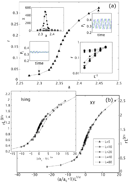
Figure 2: (a) Onset of synchronization in $d$=3. The system size $L$=80 is used. Upper left inset: Fluctuations peak near the critical point, giving an estimation of $a_{c}$=2.345$\pm$0.005. $P_{1}$ and $P_{2}$ undergo smooth temporal oscillations for large $a$ (upper right inset), while lower $a$ decreases temporal coherence (lower left inset). Lower right inset: Log-log plots of $r$ vs $L^{-1}$ with $a$=2.275, 2.3, 2.325, 2.375, 2.4, 2.425 from lowest to highest plots. (b) Finite size scaling analysis for $d$=3 using the XY and Ising critical exponents. Data collapse with $a_{c}$=2.345.

The interesting behavior emerges when the transition probability of a given unit to the state ahead depends on the states of the unit’s nearest neighbors in a spatial grid. To capture the physical nature of synchronization, we choose a function which compares the phase at a given site with its neighbors, and adjusts the phase at the given site so as to facilitate phase coherence. With universality in mind, we stress that the specific nature of the coupling is not important so long as we ultimately observe a transition to global synchrony at some finite value of the coupling parameter. For any unit, the transition rate from state $i$ to state $j$ is given by

$$g_{ij}=g\exp\left[{\frac{a(N_{j}-N_{i})}{2d}}\right]\delta_{j,i+1},$$ (2)

where the constant $a$ is the coupling parameter and $\delta$ is the Kronecker delta. $N_{k}$ is the number of nearest neighbors in state $k$, and $2d$ is the total number of nearest neighbors in $d$ dimensional cubic lattices. While this choice is by no means unique and these rates are somewhat distorted by their independence of the number of nearest neighbors in state $i-1$, the form (2) is simplified by this assumption and, as we shall see, does lead to synchronization.

To test for the emergence of global synchrony, we first consider a mean field version of the model. In the large $N$ limit with all-to-all coupling we write

$$g_{ij}=g\exp\left[a(P_{j}-P_{i})\right]\delta_{j,i+1}.$$ (3)

Note that in the mean field limit $g_{ij}$ does not depend on the location of the unit within the lattice. Also, there is an inherent assumption that we can replace $N_{k}/N$ with $P_{k}$. With this simplification we arrive at a nonlinear equation for the mean field probability, $\partial P(t)/\partial t=M[P(t)]P(t)$, with

$$M[P(t)]=\begin{pmatrix}-g_{12}&0&g_{31}\\ g_{12}&-g_{23}&0\\ 0&g_{23}&-g_{31}\end{pmatrix}.$$ (4)

Normalization allows us to eliminate $P_{3}$ and obtain a closed set of equations for $P_{1}$ and $P_{2}$. We can further characterize the mean field solutions by linearizing about the fixed point $(P_{1}^{*},P_{2}^{*})=(1/3,1/3)$. The complex conjugate eigenvalues of the Jacobian evaluated at the fixed point, $\lambda_{\pm}=g(2a-3\pm i\sqrt{3})/2$, cross the imaginary axis at $a=1.5$, indicative of a Hopf bifurcation at this value, which following a more detailed analysis kuznetsov can be shown to be supercritical. Hence, as $a$ increases, the mean field undergoes a qualitative change from disorder to global oscillations, and the desired global synchrony emerges. Numerical solutions confirm this behavior, yielding results that agree with simulations of an all-to-all coupling array ourlongerpaper . Here we characterize the breakdown of the mean field description for the nearest-neighbor coupling model as spatial dimension is decreased.

We perform simulations of the locally coupled model in continuous time on $d$-dimensional cubic lattices with periodic boundary conditions. Time steps are 10 to 100 times smaller than the fastest local average transition rate, i.e., $dt\ll e^{-a}$ (we set $g$=1). We find that much smaller time steps lead to essentially the same results. Starting from random initial conditions, all simulations were run until an apparent steady state was reached, and statistics are based on 100 independent trials.

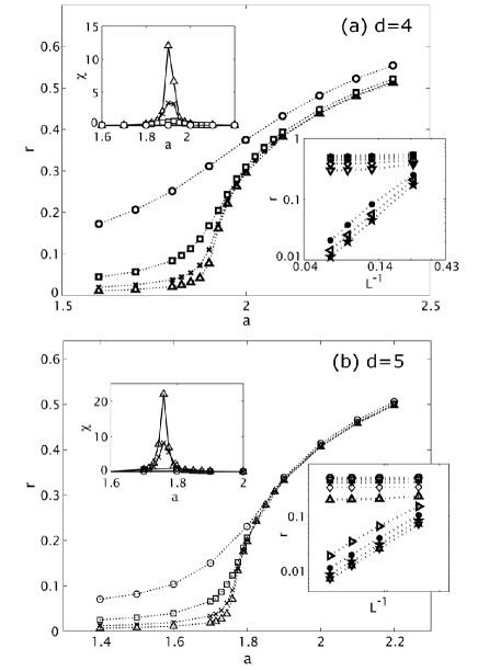
Figure 3: Transition in $d$=4 (top) and $d$=5 (bottom): The order parameter near the transition point is shown for various system sizes. $\bigcirc~{}L$=4, $\square~{}L$=8, $\times~{}L$=12, $\triangle~{}L$=16 for $d$=4 and $\bigcirc~{}L$=4, $\square~{}L$=6, $\times~{}L$=8, $\triangle~{}L$=10 for $d$=5. The upper left inset in each panel shows the generalized susceptibility which peaks at $a$=1.900$\pm$0.025 for $d$=4 and at $a$=1.750$\pm$0.015 for $d$=5. The lower right inset shows the system size dependence of the order parameter. For $d$=4 the coupling constant varies from $a$=1.6 to 2.4 in increments of 0.1 (excluding $a$=1.9) from lowest to highest plots and for $d$=5 from $a$=1.4 to 2.2 in increments of 0.1.

To characterize the emergence of phase synchrony, we introduce the order parameter kuramoto

$$r=\langle R\rangle,\quad R\equiv\frac{1}{N}\left\lvert\sum_{j=1}^{N}e^{i\phi_{j}}\right\rvert.$$ (5)

Here $\phi_{j}$ is the discrete phase 2$\pi$($k$-1)/3 for state $k\in\{1,2,3\}$ at site $j$. The brackets represent an average over time in the steady state and over all independent trials. Nonzero $r$ in the thermodynamic limit indicates synchrony. We also calculate the generalized susceptibility $\chi=L^{d}[\langle R^{2}\rangle-\langle R\rangle^{2}]$.

In $d$=2 we do not see the emergence of global oscillatory behavior. Instead, we observe intermittent oscillations (for very large values of $a$) that decrease drastically with increasing system size. In fact, $r\rightarrow 0$ in the thermodynamic limit, even for very large values of $a$ ourlongerpaper . We conclude that the phase transition to synchrony cannot occur for $d$=2. Interestingly, snapshots of the system reveal increased spatial clustering as $a$ is increased, as well as the presence of defect structures, perhaps indicative of Kosterlitz-Thouless-type phenomena goldenfeld . Further studies along these lines are underway.

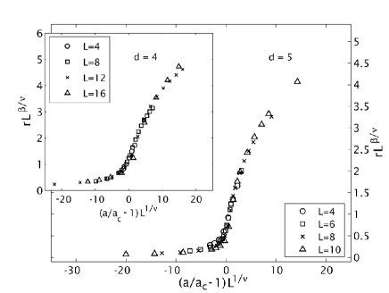
Figure 4: Finite size scaling analysis for $d$=4 and $d$=5: Data collapse using ansatz (6) with mean field exponents.

In contrast to the $d$=2 case, which serves as the lower critical dimension, a clear thermodynamic-like phase transition occurs in three dimensions. We see the emergence of global oscillatory behavior as $a$ increases past a critical value $a_{c}$. Figure 2a shows the behavior of the order parameter as $a$ is increased for the largest system studied ($L$=80); the upper left inset shows the peak in $\chi$ at $a$=2.345$\pm$0.005, thus providing an estimate of the critical point $a_{c}$. We see no change as system size is increased beyond $L$=40. At any rate, finite size effects are within the range of our estimation. The lower right inset in Fig. 2a shows explicitly that for $a<a_{c}$, $r\rightarrow 0$ as system size is increased, and a disordered phase persists in the thermodynamic limit. For $a>a_{c}$, the order parameter approaches a finite value as the system size increases. We tried to apply the Binder cumulant crossing method binder for determining $a_{c}$ more precisely, but residual finite size effects and statistical uncertainties in the data prevent us from determining the crossing point with more precision than that stated above. In any case, the accuracy of our current estimation of the critical point suffices to determine the universality class of the transition.

To further characterize this transition, we use finite size scaling analysis by assuming the standard scaling

$$r=L^{-\frac{\beta}{\nu}}F[(a-a_{c})L^{\frac{1}{\nu}}].$$ (6)

Here $F(x)$ is a scaling function that approaches a constant as $x\rightarrow 0$. To test our numerical data against different universality classes we choose the appropriate critical exponents for each, recognizing that there are variations in the reported values of these exponents pelissetto . For the XY universality class we use the exponents $\beta$=0.34 and $\nu$=0.66 gottlob . For the Ising exponents we use $\beta$=0.31 and $\nu$=0.64 huang . In Fig. 2b, we see quite convincingly a collapse when exponents from the XY class are used. For comparison, we also show the data collapse with 3D Ising exponents (note the scale differences).

For $d$=4 we estimate the transition coupling to be $a_{c}$=1.900$\pm$0.025 from the peak in $\chi$ (Fig. 3a). Because we expect $d$=4 to be the upper critical dimension in accordance with XY/Ising behavior, we anticipate a slight breakdown of the scaling relation (6). A priori it is not clear how strongly (6) will be violated in $d$=4. As shown in Fig. 4, the data collapse is very good with the mean field exponents. As such, our simulations suggest that $d$=4 serves as the upper critical dimension; additionally, it appears that corrections to finite-size scaling at $d$=4 are not substantial, though a much more precise study would be needed to investigate such corrections in greater detail.

To further support the claim that $d_{uc}$=4, we consider the case $d$=5. We see a transition to synchrony at $a_{c}$=1.750$\pm$0.015 (Fig. 3b). As expected, this value is considerably closer than the critical coupling in four dimensions to the mean field value $a_{c}$=1.5. The data collapse with the mean field exponents is excellent, as shown in Fig. 4. We note the rarity of computations in such a high dimension.

In conclusion, while nonequilibrium phase transitions exhibit a much wider diversity in universality classes than equilibrium ones net , it is remarkable that the prototype of a nonequilibrium transition, namely, a phase transition that breaks the symmetry of translation in time, is described by an equilibrium universality class. In particular, the Mermin-Wagner theorem, stating that continuous symmetries can not be broken in dimension two or lower, appears to apply. The XY model is known to display a Kosterlitz-Thouless transition in which, beyond a critical temperature, vortex pairs can unbind into individual units creating long range correlations. Preliminary results indicate that a similar transition occurs in our model.

Finally, a note of caution concerning the discreteness of the phase is in order. We first note that microscopic models often feature discrete degrees of freedom. For example, our model is reminiscent of the triangular reaction model of Onsager onsager , on the basis of which he illustrated the concept of detailed balance as a characterization of equilibrium. Continuous phase models appear in a suitable thermodynamic limit. We stress that the breaking of time translational symmetry can occur independently of whether the phase is a discrete or continuous variable. It is, however, not evident whether continuous and discrete phase models belong to the same universality class. For example, the three state ferromagnetic Potts model displays a weak first order phase transition in $d$=3 potts , while the anti-ferromagnetic version belongs to the XY universality class pelissetto ; antipotts . The results found here appear to be compatible with the latter, but a renormalization calculation confirming this hypothesis would be welcome.

References

- (1) S. H. Strogatz, Nonlinear Dynamics and Chaos (Westview Press, 1994); A. Pikovsky, M. Rosenblum, J. Kurths, Synchronization (Cambridge Univ. Press, Cambridge, 2001).
- (2) S. H. Strogatz, Physica D 143, 1 (2000); J. A. Acebón et al., Rev. Mod. Phys. 77, 137 (2005).
- (3) H. Sakaguchi, S. Shinomoto, and Y. Kuramoto, Prog. Theor. Phys. 77, 1005 (1987); H. Daido, Phys. Rev. Lett. 61, 231 (1988); S. H. Strogatz and R. E. Mirollo, J. Phys. A 21, L699 (1988); idem, Physica D 31, 143 (1988); H. Hong, H. Park, and M. Choi, Phys. Rev. E 71, 054204 (2004).
- (4) T. Risler, J. Prost, F. Jülicher. Phys. Rev. Lett. 93, 175702 (2004); Phys. Rev. E 72, 016130 (2005).
- (5) N. Goldenfeld, Lectures on Phase Transitions and the Renormalization Group (Westview Press, 1992).
- (6) T. Prager, B. Naundorf, and L. Schimansky-Geier, Physica A 325, 176 (2003).
- (7) Yu. A. Kuznetsov, Elements of Applied Bifurcation Theory, 2nd ed. (Springer, New York, 1998).
- (8) K. Wood, C. Van den Broeck, R. Kawai, and K. Lindenberg, in preparation.
- (9) K. Binder, Z. Phys. B 43, 119 (1981).
- (10) A. Pelissetto and E. Vicari, Phys. Rep. 368, 549 (2002).
- (11) A. P. Gottlob and M. Hasenbusch, Nucl. Phys. B Suppl. 30, 838 (1993).
- (12) K. Huang, Statistical Mechanics Second Edition (Wiley, New York, 1988).
- (13) See, e.g., J. Marro and R. Dickman, Nonequilibrium Phase Transitions in Lattice Models (Cambridge Univ. Press, Cambridge, 1999); V. Privman, Nonequilibrium Statistical Mechanics in One Dimension (Cambridge Univ. Press, Cambridge, 1997).
- (14) L. Onsager, Phys. Rev. 37, 405 (1931);, ibid 38, 2265(1931).
- (15) W. Janke and R. Villanova, Nucl. Phys. B 489, 679 (1997).
- (16) A. P. Gottlob and M. Hasenbusch, Physica A 210, 217 (1994); M. Kolesik and M. Suzuki, Physica A 216, 469 (1995).