A new class of exact solitary wave solutions of one dimensional Gross-Pitaevskii equation

Abstract

We present a large family of exact solitary wave solutions of the one dimensional Gross-Pitaevskii equation, with time-varying scattering length and gain/loss, in both expulsive and regular parabolic confinement regimes. The consistency condition governing the soliton profiles is shown to map on to a linear Schrödinger eigenvalue problem, thereby enabling one to find analytically the effect of a wide variety of temporal variations in the control parameters, which are experimentally realizable. Corresponding to each solvable quantum mechanical system, one can identify a soliton configuration. These include soliton trains in close analogy to experimental observations of Strecker et al., [Nature 417, 150 (2002)], spatio-temporal dynamics, solitons undergoing rapid amplification, collapse and revival of condensates and analytical expression of two-soliton bound states, to name a few.

Coherent atom optics is the subject of much current interest due to its relevance to both fundamental aspects of physics, as well as to technology Lenz ; Cornell ; Kett ; Busch ; Gupta ; Bloch . For that purpose, lower dimensional condensates e.g., cigar-shaped Bose-Einstein condensates (BECs) have been the subject of active study in the last few years Garcia ; Stringari ; Carr1 ; Liang ; Konotop . Observations of dark and bright solitons Burger ; Khaykovich ; Strecker , particularly the latter one, since the same is a condensate itself, have generated considerable interest in this area. This has spurred intense investigations about the behavior of condensates in the presence of time-varying control parameters. These include nonlinearity, achievable through Feshbach resonance Vogels ; Kett1 ; Wieman , gain/loss and the oscillator frequency Bigelow . The fact that for a condensate in oscillator potential, exact solutions of the Gross-Pitaevskii (GP) equation are not available, makes it extremely difficult to examine the effects of time variation in the aforementioned parameters. In the context of pulse propagation in non-linear optical fibers, a number of authors have recently investigated the effects of variable non-linearity, dispersion and gain or loss. Moores analyzed this problem for constant dispersion and nonlinearity and a distributed gain Moores , whereas Kruglov et al., considered the same problem with all the parameters in a variable form Kruglov . Serkin et al., have derived the nonlinear Schrödinger equation (NLSE) with distributed coefficients as compatibility condition of two first order equations, demonstrating the applicability of inverse scattering transform method to this type of problems HaseIEEE . They write down the general equation relating the distributed coefficients with the solution parameters and obtain a number of exact solutions. Recently, exact solutions of a driven NLSE with distributed dispersion, nonlinearity and gain, which exhibits pulse compression in a twin-core optical fiber, has also been obtained PKP1 .

In this Letter, we present a large family of exact solutions of the quasi one-dimensional GP equation, which is the familiar NLSE, with time varying scattering length, gain/loss, in the presence of an oscillator potential, which can be both expulsive or regular. It is shown that, the consistency condition governing the soliton profiles identically maps on to the linear Schrödinger eigenvalue problem, thereby allowing one to solve analytically the GP equation for a wide variety of temporal variations in the control parameters. Corresponding to each solvable quantum mechanical eigenvalue problem, one can identify a soliton-like profile. These can be dark or bright and the oscillator frequencies can have a variety of temporal profiles, including linear, quadratic, exponential, smooth step-like potential and kicked oscillator scenario. Our solutions exhibit soliton trains, spatio-temporal dynamics of solitons, the formation of two-soliton bound states, to name a few. Interestingly, it was found that some of these solitons can periodically exchange atoms with a background. Further, our analytical results are closely related to experiments Khaykovich ; Strecker . Amplification of atomic condensate and condensate compression are observed in the parameter domain, which are amenable for experimental verification.

Analogous to the experimental observations of Strecker et al., we obtain bright soliton trains in the presence of harmonic confinement Strecker . Some of the soliton solutions in the presence of regular harmonic confinement, with appropriately tailored gain/loss, exhibit collapse and revival phenomena, with an increase in amplitude. We treat the attractive regime rather exhaustively since the bright solitons are themselves condensates. The analytic expression for the dark soliton in the repulsive sector has been presented, detailed analysis of the same can be carried out in a straightforward manner.

We start with a zero temperature BEC of atoms, confined in cylindrical harmonic trap $V_{0}(x,y)=m\omega_{\perp}^{2}(x^{2}+y^{2})/2$ and a time-dependent harmonic confinement, which can be both attractive and expulsive, along the $z$-direction $V_{1}(z,t)=m\omega_{0}^{2}(t)z^{2}/2$:

$$i\hbar\frac{\partial\Psi({\bf{r}},t)}{\partial t}=\left\{-\frac{\hbar^{2}}{2m}\nabla^{2}+U|\Psi({\bf{r}},t)|^{2}+V+i\frac{\eta(t)}{2}\right\}\Psi({\bf{r}},t),$$ (1)

where $U=4\pi\hbar^{2}a_{s}(t)/m$ and $V=V_{0}+V_{1}$. It is worth noting that, condensate can interact with the normal atomic cloud through three-body interaction, which can be phenomenologically incorporated by a gain/loss term $\eta(t)$.

To reduce Eq.(1) to an effective one dimensional equation, we assume that, the interaction energy of atoms is much less than the kinetic energy in the transverse direction Salasch :

$$\Psi({\bf{r}},t)=\frac{1}{{\sqrt{2\pi a_{B}}}a_{\perp}}\psi\left(\frac{z}{a_{\perp}},\omega_{\perp}t\right)$$

$$\times\exp\left(-i\omega_{\perp}t-\frac{x^{2}+y^{2}}{2a_{\perp}^{2}}\right)~{}.$$ (2)

In dimensionless units, GP equation then reduces to the following one dimensional nonlinear Schrödinger equation:

$$i\partial_{t}\psi=-\frac{1}{2}\partial_{zz}\psi+\gamma(t)|\psi|^{2}\psi+\frac{1}{2}M(t)z^{2}\psi+i\frac{g(t)}{2}\psi~{}.$$ (3)

Here, $\gamma=2a_{s}(t)/a_{B}$, $M(t)=\omega_{0}^{2}(t)/\omega_{\perp}^{2}$, $g(t)=\eta(t)/\hbar\omega_{\perp}$, $a_{\perp}=(\hbar/m\omega_{\perp})^{1/2}$ and $a_{B}$ is the Bohr’s radius. For the sake of generality we have kept $M(t)$ time dependent, a constant $M(t)$ implies an oscillator potential which can be confining or expulsive for $M>0$ or $M<0$, respectively.

In order to discuss the cases of a variety of experimentally achievable profiles of the time dependent trapping potential and to obtain corresponding analytical solutions, we assume the following ansatz solution:

$$\psi(z,t)=\sqrt{A(t)}F[A(t)\left\{z-l(t)\right\}]\exp[i\Phi(z,t)+G(t)/2],$$ (4)

where, $G(t)=\int_{0}^{t}g(t^{\prime})dt^{\prime}$, $l(t)=\int_{0}^{t}v(t^{\prime})dt^{\prime}$ and we assume that phase has a quadratic form:

$$\Phi(z,t)=a(t)+b(t)z-\frac{1}{2}c(t)z^{2}.$$ (5)

In the above equation, $a(t)=a_{0}+\frac{\lambda-1}{2}\int_{0}^{t}A^{2}(t^{\prime})dt^{\prime}$, and $c(t)$ is determined by a Riccati type equation:

$$c_{t}-c^{2}(t)=M(t).$$ (6)

Interestingly, this equation can be expressed as a Schrödinger eigenvalue problem via a change of variable, $c(t)=-\frac{d\ln[\varphi(t)]}{dt}$:

$$-\varphi^{\prime\prime}(t)-M(t)\varphi(t)=0.$$ (7)

Taking advantage of this connection, below we show that, corresponding to each solvable quantum mechanical system, one can identify a soliton configuration. The fact that, Schrödinger equation can be exactly solved for a variety of $V(t)$, gives us freedom to control the dynamics of BEC in a number of analytically tractable ways. This is one of the main results of this Letter. Although a host of time dependent oscillator frequencies can be addressed, we will only demonstrate in the text, a few experimentally realizable examples.

We also find the following consistency conditions

$$\left.\begin{array}[]{c}\gamma(t)=\gamma_{0}e^{-G(t)/2}A(t)/A_{0},~{}~{}b(t)=A(t)\\ A(t)=A_{0}\exp\left\{\int_{0}^{t}c(t^{\prime})dt^{\prime}\right\},~{}~{}A_{0}>0\\ \frac{dl(t)}{dt}-c(t)l(t)=b(t)\end{array}\right\}$$ (8)

Now substitution of the ansatz Eq. (4) in Eq. (3) and using the consistency conditions Eq.(8), we obtain the differential equation for the function $F$ in terms of the new variable $T=A(t)[z-l(t)]$:

$$F^{\prime\prime}(T)-\lambda F(T)+2\kappa F^{3}(T)=0,~{}{\mathrm{where}}~{}\kappa=-\frac{\gamma_{0}}{A_{0}}.$$ (9)

We note that, the Eq. (9) possesses a variety of solutions in the form of twelve Jacobian elliptic functions e.g., $\mathrm{cn}(T,m)$, $\mathrm{sn}(T,m)$ and $\mathrm{dn}(T,m)$ etc. Here $m$ is the modulus parameter taking value in the interval $0\leq m\leq 1$. These functions interpolate between the trigonometric and hyperbolic functions in the limiting cases $m=0$ and $1$, respectively. In the appropriate parameter regimes, a wide variety of solutions emerge which include soliton trains, akin to experimental observations of Strecker et al., and localized bright and dark solitons.

The bright soliton trains of the form $\psi(z,t)=\sqrt{A(t)}{\mathrm{cn}}\left[T/\tau_{0},m\right]\exp[i\Phi(z,t)+G(t)/2]$ exist for $\kappa>0$, where $\tau_{0}^{2}=-A_{0}(m+m^{2})/2\gamma_{0}$ and $\lambda=(m^{2}+m-1)/2\tau_{0}^{2}$. Here, all the coefficients are determined from Eqs. (5-8). It should be pointed out that, in the repulsive domain $\gamma_{0}>0$ the localized dark soliton is of the form $\psi(z,t)=\sqrt{A(t)}\tanh\left[\frac{A(t)z}{\tau_{0}}\right]\exp[i\Phi(z,t)+G(t)/2],$ since the same vanishes at the origin. The cnoidal wave solution for this is of $\mathrm{sn}(T,m)$ type.

Below, we examine the formation and dynamics of nonlinear excitations in the presence of an oscillator potential, with a variety of experimentally achievable temporal modulations in the frequency.

Soliton trains in a confining oscillator.— Inspired by the experiments of Strecker et.al, Strecker in the presence of confining oscillator, with no gain/loss we obtain following moving soliton trains with velocity $v(t)=A_{0}\cos(M_{0}t)$:

$$\psi(z,t) = \sqrt{A_{0}\sec(M_{0}t)}$$ (10)

$$\times {\mathrm{cn}}\left[\frac{A_{0}\sec(M_{0}t)(z-\frac{A_{0}}{M_{0}}\sin[M_{0}t])}{\tau_{0}},m\right]e^{i\Phi}.$$

As shown in Fig. (1) initially at $\approx 5ms$ there is only one profile and as time progresses it breaks up in to many profiles giving rise to a soliton train.

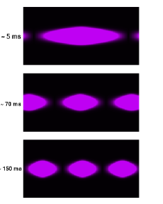
Figure 1: Plots depicting the snapshots of soliton trains at times $\approx 5ms$, $\approx 70ms$ and $\approx 150ms$ with parameters $M=.25$, $\gamma=-0.5$, $\tau_{0}=.9999$, $A_{0}=0.5$ and modulus parameter $m=.99999$.

Collapse and revival of the condensate.— Inspired by the experiments of Strecker et al., we tailor the gain profile in the same range of the parameters, where one observes dramatic collapse and revival of condensates with an increase in the amplitude. Specifically we take, $M(t)=M_{0}^{2}$, $g(t)=a_{1}t-a_{2}\sin(\delta t)$ and $\gamma(t)=\gamma_{0}\exp\left[\frac{-a_{1}t^{2}}{2}-\frac{a_{2}}{\delta}\cos(\delta t)\right]\sec(M_{0}t)$, for which we obtain from Eq. (8), $A(t)=A_{0}\sec(M_{0}t)$. The complete solution can be written as

$$\psi(z,t)=\sqrt{A_{0}\sec(M_{0}t)}\mathrm{sech}\left[\frac{A_{0}\sec(M_{0}t)z}{\tau_{0}}\right]\exp\left[G(t)/2\right]e^{i\Phi}.$$ (11)

This is depicted in Fig.(2). In this case, sinusoidal nature of gain function implies a periodic exchange of atoms with the background. In the attractive domain, presence of a background surrounding the condensate has been seen in the experiments leading to formation of bright solitons Strecker ; Khaykovich . In this light, the collapse and revival of the condensate, having a sinusoidal exchange of atoms with the background, may be amenable for verification.

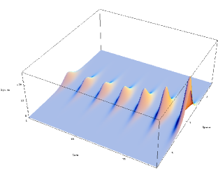
Figure 2: Figure depicting collapse and revival of atomic condensate and amplification through periodic exchange of atoms with the background, for the parameter values $M=0.0025$, $\tau_{0}=2.5$, $A_{0}=3.125$, $\gamma_{0}=-0.5$ as in the Ref. Strecker and gain parameters $a_{1}=.01$, $a_{2}=8.25$ and $\delta=1.5$.

Soliton formation from step changes in the trap potential.— Below, we explicate in the attractive domain ($\gamma_{0}<0$) the effect of a step like change in the oscillator frequency which is well mimicked by the function $M(t)=-4+\frac{3}{2}[1+\tanh(t/2)]$, for which the coupling has the form $\gamma(t)=\gamma_{0}\left[\frac{e^{2t}}{(1+e^{t})}\right]$, $\gamma_{0}<0$. As time progresses, the coupling strength changes exponentially and the condensate wave function starts building up rapidly. In this expulsive case, like the experimentally observed bright soliton Khaykovich , one obtains,

$$\psi(z,t)={\sqrt{\frac{A_{0}e^{2t}}{(1+e^{t})}}}\mathrm{sech}\left[\frac{A_{0}e^{2t}z}{(1+e^{t})\tau_{0}}\right]\exp[i\Phi(z,t)].$$ (12)

New solutions in the case of constant coupling.— A number of interesting condensate profiles emerge in the constant attractive coupling regime, depending on the nature of the external potential. For the regular oscillator confinement one obtains a spectacular spatio-temporal pattern given by Eq. (13) in the amplitude of the order parameter, as seen in Fig. (3). The extreme increase in amplitude happens due to the presence of the $\sec(M_{0}t)$ in the amplitude.

$$\psi(z,t)=\sqrt{A_{0}\sec(M_{0}t)}\mathrm{sech}\left[\frac{A_{0}\sec(M_{0}t)}{\tau_{0}}\right]\exp[G/2]e^{i\Phi}$$ (13)

New bound state for solitons.—Interestingly, as shown in Fig. (4), in the expulsive domain one obtains bound states of solitons in the same parameter regime. The analytical expression for this remains same as in Eq.(13), except for the value of $A(t)$ which is now given by$A(t)=A_{0}\mathrm{sech}[M_{0}t]$. It is worth mentioning that, in optical fibers with a variable dispersion similar structures have been seen through numerical investigations Kumar .

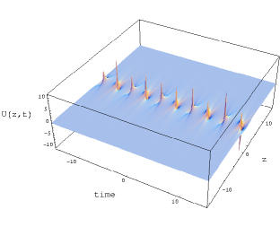
Figure 3: Figure depicting spatio-temporal pattern of condensate wave function in a confining oscillator potential ($M(t)=0.25$) with constant attractive coupling $\gamma(t)=-0.5$ and $A_{0}=0.5$, $\tau_{0}=1$.

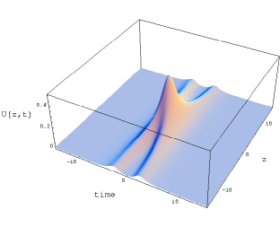
Figure 4: Formation of two-soliton bound state in an expulsive potential($M(t)=-0.25$) with all the other parameters having same values as in Fig.(3).

Keeping in mind, the nontrivial nature of the phase and its connection with soliton profile, the nature of the spatio-temporal dynamics of the same for various configurations is worth discussing. The quadratic nature of the phase with respect to the space coordinate introduces a spatial chirping effect. Furthermore, its coefficient $c(t)$ is also time-dependent and is connected with the external potential through Eq. (6); hence the trap potential has a signature on the same. The purely temporal part $a(t)$ is also sensitive to trap potential as depicted by Eq. (8).

In conclusion, for one dimensional GP equation in an oscillator potential, with time dependent coupling and gain/loss, we have obtained a wide class of exact solutions. These include experimentally observed bright soliton profile in the attractive coupling regime for the expulsive case. The fact that the equation governing the soliton profiles in the presence of time dependent harmonic oscillator, maps to the Schrödinger equation, opens up a host of opportunities. Corresponding to any solvable quantum mechanical potential, a time dependent cigar-shaped BEC profile can be obtained. We have explicated amplification of BEC profile through smooth variation of the oscillator frequency. Formation of soliton bound states and spectacular spatio-temporal patterns that can manifest in this nonlinear system with time-dependent control parameters are demonstrated. One observes dramatic compression and localization of broad condensate profiles, which may have technological implications. We have analyzed the nonlinear excitations in the presence of oscillator potential having linear, quadratic, Morse and other type of time dependencies.

References

- (1) G. Lenz, P. Meystre, and E.M. Wright, Phys. Rev. Lett. 71, 3271 (1993).
-
(2)
Y.J. Wang et al., Phys. Rev. Lett. 94, 090405 (2005);
Y. Shin et al., Interference of Bose-Einstein Condensates on an Atom Chip, cond-mat/0506464. - (3) Th. Busch et al., Phys. Rev. A 65, 043615 (2002).
- (4) S. Gupta, K. Dieckmann, Z. Hadzibabic, and D. E. Pritchard, Phys. Rev. Lett. 89, 140401 (2002).
- (5) I. Bloch, T.W. Hänsch, and T. Esslinger, Phys. Rev. Lett. 82, 3008 (1999).
- (6) W. Ketterle, Rev. Mod. Phys. 74, 1131 (2002).
- (7) V.M. Pérez-Garcia, H. Michinel and H. Herrero, Phys. Rev. A 57, 3837 (1998).
- (8) F. Dalafovo et al., Rev. Mod. Phys. 71, 463 (1999).
- (9) S. Burger et al., Phys. Rev. A 65, 043611 (2002); L.D. Carr et al., Phys. Rev. A 62, 063610 (2000); L.D. Carr and Y. Castin, Phys. Rev. A 66, 063602 (2002); L.D. Carr, M.A. Leung and W.P. Reinhardt, J. Phys. B: At. Mol. Opt. Phys. 33, 3983 (2000).
- (10) Z.X. Liang, Z.D. Zhang and W.M. Liu, Phys. Rev. Lett. 94, 050402 (2005).
- (11) V. Konotop and P. Pacciani, Phys. Rev. Lett. 94, 240405 (2005).
- (12) F.S. Cataliotti et al., Science 293, 843 (2001).
- (13) L. Khaykovich et al., Science 296, 1290 (2002).
- (14) K.E. Strecker et al., Nature 417, 150 (2002); U. Al Khawaja et al., Phys. Rev. Lett. 89, 200404 (2002).
- (15) J.M. Vogels et al., Phys. Rev. A 56, R1067 (1997).
- (16) S. Inouye et al., Nature 392, 151 (1998).
- (17) J.L. Roberts et al., Phys. Rev. Lett. 85, 728 (2000).
- (18) J. Janis, M. Banks and N.P. Bigelow, Phys. Rev. A 71, 013422 (2005).
- (19) J.D. Moores, Opt. Lett. 21, 555 (1996).
- (20) V.I. Kruglov, A.C. Peacock and J.D. Harvey, Phys. Rev. Lett. 90, 113902 (2003).
-
(21)
V.N. Serkin and A. Hasegawa, IEEE J. Sel. Top. Quantum Electron. 8, 418 (2002);
V.N. Serkin, A. Hasegawa, and T.L. Belyaeva, Phys. Rev. Lett. 92, 199401 (2004). - (22) T.S. Raju, C.N. Kumar and P.K. Panigrahi, J. Phys. A: Math. Gen. 38, L271 (2005); T.S. Raju, P.K. Panigrahi and K. Porsezian, Phys. Rev. E 71, 026608 (2005).
- (23) L. Salasnich, A. Parola and L. Reatto, Phys. Rev. A 65, 043614 (2002).
- (24) S. Kumar and A. Hasegawa Opt. Lett. 22, 372 (1997); V.N. Serkin and A. Hasegawa, Phys. Rev. Lett. 85, 4502 (2002).