Harmonic vibrational excitations in graded elastic networks: transition from phonons to gradons

Abstract

We have identified a new type of transition from extended to localized vibrational states in one-dimensional graded elastic chains of coupled harmonic oscillators, in which the vibrating masses or nearest-coupling force constants vary linearly along the chain. We found that the delocalization transition occurs at the maximum frequency of the corresponding homogeneous chain, which is in a continuous single band. Although each state in the localized phase, called gradon, can be regarded as an impurity localized mode, the localization profile is clearly distinct from usual impurity modes or the Anderson localized modes. We also argue how gradons may affect the macroscopic properties of graded systems. Our results can provide insights into many analogous systems with graded characters.

I Introduction

Vibrational normal modes and their localization properties in inhomogeneous or disordered media have attracted much interest. Lieb68 ; Wallis68 ; Yip84 ; Tamura88 ; Yakubo03 ; Chan04 Notable examples include disorder-induced localized states (i.e., the Anderson localization of lattice vibrations), fractal-induced localization (i.e., fractons YakuboRMP ), modes contributing the boson peak, Kantelhardt01 the connection of excess of low-frequency modes with the jamming-unjamming transition in particle packings, Silbert05 intrinsic localized modes (ILMs) caused by nonlinearity and/or discreteness in systems, Campbell04 and the well-known defect modes in crystals including impurities Wallis68 ; Defect etc. Surface phonon modes in semiconductors are also typical localized vibrational excitations in which atomic displacements decrease exponentially into the bulk. Fritsch99 These localized vibrational modes strongly affect properties of condensed matter. It is crucial to reveal characteristics of localized modes for understanding thermal, elastic, and acoustic properties and/or electron-phonon interactions in materials.

From the viewpoint of localization mechanisms, there exist two types of localized modes in noninteracting systems. The first type is a consequence of interference of coherent vibrational waves due to diffusive scattering. Localized modes of this type include the Anderson localization of classical waves Stephen83 ; PSheng95 and fractons in fractal systems. YakuboRMP In these cases, localization occurs whenever the elastic mean free path becomes comparable to the inverse wave vector of the wave (the Ioffe-Regel condition). In particular, the Anderson localization of elastic waves in disordered solids has been extensively studied theoretically and experimentally. Elliott03 ; Feddersen91 ; Foret96 Now, we have obtained vast amount of knowledge on the Anderson localization and the Anderson transition, which involve similarities to and differences from quantum particle localization. Brandes04 The mode pattern of an Anderson localized state possesses an exponential tail and the position of the localization center is unpredictable. The scaling theory Abrahams79 shows all vibrational modes are localized in one- and two-dimensional disordered systems while one has the localization-delocalization transition in three dimensions, which is the same with the Anderson transition of quantum particles in the orthogonal universality class. Mehta91 The delocalization transition occurs in a continuous band without any singularity of the spectrum at the transition frequency $\omega_{\text{c}}$. The localization length $\xi$ diverges as a power law of $|\omega-\omega_{\text{c}}|$. The other type of localizations is due to confinement by impurities such as defect modes, surface modes, or ILMs. Maradudin71 This type of localized modes is rather trapped by local potentials. The mode pattern of such an impurity localized mode has also an exponential tail and the position of the localization center is located at the impurity site. For instance, the light-mass impurity mode of a one-dimensional elastic chain has the mode pattern of $u_{n}\propto[-m_{0}/(2m-m_{0})]^{|n|}$, where $m$ and $m_{0}$($<m$) are the host and impurity masses, respectively, and $n$ is the site number ($n=0$ represents the impurity site). The frequency of this light-mass impurity mode is given by $\omega_{\text{imp}}^{2}=m^{2}\omega_{\text{max}}^{2}/m_{0}(2m-m_{0})$, where $\omega_{\text{max}}$ is the maximum frequency of the homogeneous chain with mass $m$ for all sites. Since $m_{0}<m$, $\omega_{\text{imp}}$ is always larger than $\omega_{\text{max}}$, which implies that the light-mass impurity localized mode has an isolated spectrum outside of the band. This is considered as a common feature of impurity localized modes. Therefore, it seems that no localization-delocalization transition induced by impurities occurs in a single band. This is, however, not obvious. If a delocalization transition in a continuous spectrum is realized by impurity modes, properties of localized vibrations and the transition would be quite different from those for conventional localized modes and transitions.

In this work, we consider vibrational problems of a graded elastic systems which are modelled by graded spring-mass networks. Studying one-dimensional (1D) systems with graded masses and graded force constants, we show a new type of transition from extended to impurity localized modes. Some characteristic properties of these localized modes are also elucidated. Graded elastic systems can be found everywhere in nature. Mass density of an elastic body subject to a gravitational field is low near the top of the object but high near the bottom, such as sediment at the bottom of ocean, which can be regarded as an example of graded elastic systems. Similar localized modes to our results can be expected in it. A carbon nanotube which can be regarded as folding a graphite sheet into a tube is another example of graded elastic materials. Mele05 The force constant can be stronger at the central part of the tube but weaker at both ends. Thus there is a gradient of force constant along the nanotube. Particularly, by virtue of the analogy of the vibrational problem with many other problems, such as electromagnetic wave propagation Nakayama92 ; Nakayama97 in which the index of refraction plays the same role as the mass, one would expect similar localizations in other type of graded structures such as quantum or photonic systems. It is possible to apply our model to graded plasmonic nanoparticle chains which may find prominent applications in nanooptics. In fact, there have been many efforts directed to graded systems in both artificial composites DongPRB03 and materials in nature (e.g., biological cells HuangPRE03 ). One further notices that in contrast to a simple sharp interface, it has been studied that the presence of gradient in a interface leads to frequency-dependent properties. Vollmann04 ; Berezovski00 Although we treated 1D chains in this work, our findings form the basis for higher dimensional networks in which results are more complicated and intriguing and we will present them elsewhere. xiao

In what follows, we first briefly describe, in Sec. II, the graded elastic network model, and establish the formalism for studying eigenmodes. In Sec. III, we present our results mainly in the graded mass model and similar results are in the graded force constant model . Finally conclusions and discussions on our results are given.

II model and formalism

The elastic vibrational problem of a uniform three-dimensional system is simply modelled by a cubic lattice of harmonic oscillators where different components of the displacement decouple. Kantelhardt01 However, when there exists a uniaxial gradient of coupling constants (or masses), the equation of motion is only partially separable. Assuming that the network is periodic in the directions perpendicular to the gradient direction (e.g., $z$-axis), one reaches an effective one-dimensional problem. xiao Without loss of generality, let us start with a one-dimensional spring-mass model as depicted in Fig. 1. The mass $M_{n}$ and the spring constant $K_{n}$ connecting to the right nearest-neighbor are labelled sequently with $n=1,2,\cdots,N$. The motion of each mass is governed by the following equations Lieb68

$$M_{n}\ddot{u}_{n}=K_{n-1}(u_{n-1}-u_{n})+K_{n}(u_{n+1}-u_{n}),$$ (1)

where $u_{n}$ denotes the scalar displacement of mass $M_{n}$ at the site $n$, and the derivative $\ddot{u}_{n}$ is taken with respect to time $t$. We omit damping and further couplings to avoid complications, the inclusion of which do not change the results qualitatively. Decomposing the amplitude $u_{n}$ by the eigenvectors $\boldsymbol{e}(\lambda)$ of the mode $\lambda$ as $u_{n}=\sum_{\lambda}Q_{\lambda}(t)e_{n}(\lambda)$, where $Q_{\lambda}(t)$ is a time-dependent expansion coefficient which behaves as $Q_{\lambda}(t)\sim\exp(-i\omega_{\lambda}t)$, we simplify Eq. (1) to the eigensystem of

$$-\omega^{2}\boldsymbol{e}=\boldsymbol{T}\cdot\boldsymbol{e},$$ (2)

where the matrix $\boldsymbol{T}$ characterizes the mass-weighted coupling interactions of the neighboring masses connected by the springs that form a lattice with lattice constant $a=1$. The system size $L$ is then given by $aN$. Assuming free boundary conditions, the $N\times N$ matrix $\boldsymbol{T}$ becomes tridiagonal and with elements

$$T_{mn}=-\Big{[}\frac{(1-\delta_{n1})K_{n-1}}{M_{m}}+\frac{(1-\delta_{nN})K_{n}}{M_{m}}\Big{]}\delta_{mn}+\frac{K_{n}}{M_{m}}(\delta_{mn-1}+\delta_{mn+1}),$$ (3)

where $\delta$ is the Kronecker delta. In this regard, further incorporating the next-nearest coupling force constant $K_{n}^{\text{next}}$ results a quintuple matrix $\boldsymbol{T}$. We have also attempted periodic boundary conditions, i.e., let $M_{n}$ connected to $M_{1}$ by $K_{n}$, very similar results are observed. The nontrivial $N$ solutions of $\boldsymbol{e}$ and $\omega^{2}$ in Eq. (2) are thus determined by diagonalizing $\boldsymbol{T}$.

In this paper, we will consider two different cases in a one-dimensional network:
(1) The graded mass case with

$$M_{n}=M_{0}-C_{\text{M}}n/N,$$ (4)

and fixed $K$ [see Fig. 1(a)]. In this case, the node mass decreases linearly from the left end site $n=1$ to $n=N$.
(2) The graded force constant case with

$$K_{n}=K_{0}+C_{\text{K}}n/N$$ (5)

and fixed $M$ [see Fig. 1(b)]. Here, $M_{0}$ and $K_{0}$ are the maximum mass and the minimum force constant, and $C_{\text{M}}$ and $C_{\text{K}}$ are the gradient coefficients in the two models, respectively. Note that the conditions of $C_{\text{M}}=0$ and $C_{\text{K}}=0$ recover the homogeneous chain. It is also emphasized that our graded models can be easily extended to infinite $N$ (namely, infinite system size $L$). The infinite graded chain does not correspond to the continuum graded chain, but to the infinitesimal gradient limit.

III Numerical Results

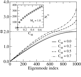
Figure 2: /Xiao, Yakubo, and Yu

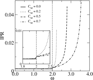
Figure 6: /Xiao, Yakubo, and Yu

In this section, we mainly concentrate on the graded mass model with $N=1000$. A further increase in $N$ does not change our results (except for Fig. 6 as shown later). The dispersion relation of the vibrational modes in a crystal gives rich information about properties of phonons. In the graded elastic network, however, the wavenumber is not conserved because of the lack of translational symmetry in the system. This does not allow us to consider the dispersion relation for our model. Nevertheless, the relation between the eigenfrequency $\omega_{\lambda}$ and the mode index $\lambda$ in ascending order with respect to $\omega_{\lambda}$, which can be regarded as a pseudo-dispersion relation, helps us to interpret vibrational modes in the graded system. Figure 2 shows the eigenfrequency $\omega_{\lambda}$ as a function of the eigenmode index $\lambda$ for gradient coefficients $C_{\text{M}}=0.0$, $0.2$, $0.5$, and $0.7$. $M_{0}=1$, $K_{0}=1$ and $C_{\text{K}}=0$ are used. Note that the relation for the homogeneous elastic chain ($C_{\text{M}}=0.0$) represents the usual dispersion relation. It is clear that the presence of the gradient alters the (pseudo-) dispersion relation, particularly beyond the frequency $\omega_{\text{c}}=2\sqrt{K_{0}/M_{0}}=2.0$ (dashed horizontal line) which is the maximum eigenfrequency of the homogeneous elastic chain with $M_{n}=M_{0}$ for any $n$ (the solid curve). The number $N_{\text{g}}$ of high-frequency excitations with $\omega>\omega_{\text{c}}$ depends on the gradient coefficient $C_{\text{M}}$ as shown by the insert of Fig. 2. The maximum frequency of the graded chain is given by $\omega_{\text{max}}=2\sqrt{K_{0}/M_{N}}$ ($2\sqrt{K_{N}/M_{0}}$) in the graded mass (force constant) model. Let us call these high energy excitations “gradons” which are clearly distinct from low frequency excitations as we will show later. The fact that $\omega_{\text{c}}$ is a characteristic frequency in the graded elastic chain is more explicitly found in the density of states (DOS) defined by

$$D(\omega)=\frac{1}{N}\sum_{\lambda}\delta(\omega-\omega_{\lambda}).$$ (6)

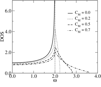
Figure 3: /Xiao, Yakubo, and Yu

The DOS shown in Fig. 3 clearly exhibits a singular maximum peak at $\omega_{\text{c}}=2.0$ for $C_{\text{M}}>0$. This behavior persists for various gradient coefficients $C_{\text{M}}$. The low-frequency DOS is in accordance with the usual asymptotic Debye density of vibrational states, both in the homogeneous case and the graded case. From the DOS, we expect that modes with $\omega>\omega_{\text{c}}$ are qualitatively different from modes with $\omega<\omega_{\text{c}}$. In order to clarify this point, we plot the mode patterns $\boldsymbol{e}(\lambda)$ in Fig. 4, where three typical modes with $\omega=2.38223(>\omega_{\text{c}})$, $1.99845(\approx\omega_{\text{c}})$, and $0.39309(<\omega_{\text{c}})$ are presented. These mode patterns show that modes with $\omega>\omega_{\text{c}}$ (namely, gradons) are confined at the “light” mass side, whereas those with $\omega<\omega_{\text{c}}$ (phonons) are extended. As will be shown later, these confined modes are qualitatively different from conventional localized modes. Nevertheless, we use the word localized modes for these confined states, because the present model exhibits a drastic change in spatial extent of modes. One can find a beating pattern in the wave profile [see Fig. 4(b)], which implies that the mode is composed of plural wavenumber components. The degree of mixing of different wavenumber components can be quantified by the full width at half maximum (FWHM) of the Fourier amplitude $|F_{j}(\boldsymbol{e})|=|\pi\sum_{n=1}^{N}e_{n}\exp{[2\pi i(j-1)(n-1)/N]}/\sqrt{N}|$. Indeed, the Fourier transform of the mode pattern in Fig. 4(a) has a finite width around the average wavenumber as shown in Fig. 5(a). Figure 5(b) gives the FWHM as a function of $\omega$ for several values of $C_{\text{M}}$. The FWHM shows singularity at $\omega=\omega_{\text{c}}$ as in the case of the DOS. For well-extended states for $\omega\ll\omega_{\text{c}}$, the FWHM must be very small, which implies that we can approximately define the Bloch wavenumber $k$ for modes in this very low frequency regime. It is then possible to regard Fig. 2 as a usual dispersion relation between $\omega$ and $k$ for $\omega\ll\omega_{\text{c}}$.

In order to quantify the degree of localization of excited modes, we consider the inverse participation ratio Toulous79 ; Wegner80 (IPR),

$$P^{-1}=\frac{\sum\limits_{n=1}^{N}e_{n}^{4}}{\Big{(}\sum\limits_{n=1}^{N}e_{n}^{2}\Big{)}^{2}}.$$ (7)

The IPR defined by Eq. (7) gives a measure of the number of sites contributing significantly to a given eigenstate. If the state is strongly localized, $P^{-1}$ becomes proportional to $1/\xi^{d}$, where $\xi$ is the localization length, while for a fairly extended state it is proportional to $1/L^{d}$ because all sites contribute to the state. We show in Fig. 6 the IPR of vibrational modes in the graded mass model as a function of the eigenfrequency for various gradient coefficients $C_{\text{M}}$. At low frequencies ($\omega<\omega_{\text{c}}$), small and almost flat IPR indicates fairly well-extended excitations across the whole network. The IPR increases dramatically, however, as the frequency exceeds $\omega_{\text{c}}=2.0$. This shows that modes with $\omega>\omega_{\text{c}}$ are spatially localized. These are in accord with the excitation shapes depicted in Fig. 4. As seen in the inset of Fig. 6, the small step of the IPR at $\omega=\omega_{\text{c}}$ is somewhat broad. This is a consequence of the finite size effect of our $N=1000$ system. We confirmed that the step becomes sharper as increasing $N$ (figure not shown here).

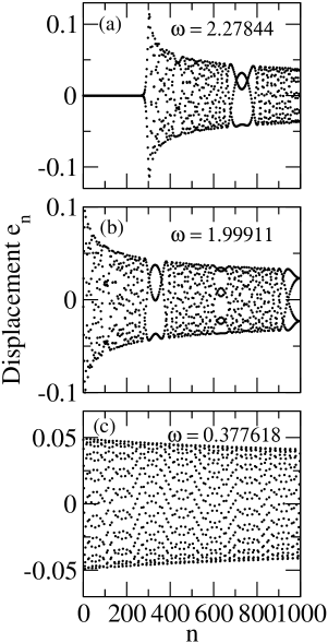
Figure 7: /Xiao, Yakubo, and Yu

Due to the duality between force constant and mass, the graded force constant model represented by Eq. (5) is essentially the same with the graded mass model we discussed above. Indeed, we basically observed the same results as those in the graded mass model. In Fig.7, for example, we present three typical excitation states with $\omega=2.27844(>\omega_{\text{c}})$, $1.99911(\approx\omega_{\text{c}})$, and $0.377618(<\omega_{\text{c}})$ for the graded force constant model with $C_{\text{K}}=1.0$. These mode patterns are quite similar to those in the graded mass model shown in Fig. 4. Further results on the pseudo-dispersion relation, the DOS, the FWHM, and the IPR show also similar behaviors to those in the graded mass case.

From all the results presented above, we can conclude that an infinite graded elastic chain exhibits the localization-delocalization transition at the frequency $\omega_{\text{c}}$ being the maximum eigenfrequency of the homogeneous elastic chain with $M_{n}=M_{0}$ (or $K_{n}=K_{0}$) for any $n$. In the frequency regime $\omega<\omega_{\text{c}}$, we have phonon-type modes extended over the whole system, while modes with $\omega>\omega_{\text{c}}$ (namely, gradons) are localized in the lighter mass side (or harder force constant side). It should be noted that this delocalization transition (the phonon-gradon transition) occurs in a single band as shown in Fig. 3. The mechanism of gradon localization is considered as follows. A mode with a frequency $\omega$ larger than $\omega_{\text{c}}$ cannot have amplitudes in the heavier (or softer) region because masses (or force constants) in this region are too heavy (or too soft) to vibrate with the frequency $\omega$. As a consequence, the mode pattern has finite amplitudes only in the lighter (or harder) region, while no amplitude in the heavier (or softer) region. The boundary between these two regions is determined by $\omega=2\sqrt{K_{n}/M_{n}}$. Therefore, the localization center site $n_{\text{c}}$ which is the position with the maximum amplitude [see Fig. 4(a)] is given by

$$n_{\text{c}}=\begin{cases}\displaystyle\frac{NM_{0}}{C_{\text{M}}}\left(1-\frac{\omega_{\text{c}}^{2}}{\omega^{2}}\right)&\text{graded mass model},\\ &\\ \displaystyle\frac{NK_{0}}{C_{\text{K}}}\left(\frac{\omega^{2}}{\omega_{\text{c}}^{2}}-1\right)&\text{graded force constant model}.\end{cases}$$ (8)

The fact that values of $n_{\text{c}}$ of the modes shown by Fig. 4(a) and Fig. 7(a) are predicted by Eq. (8) as $n_{\text{c}}=423$ for Fig. 4(a) and $298$ for Fig. 7(a) shows the validity of our interpretation of gradon localization. This mechanism of localization is essentially the same with that of impurity localized modes. Therefore, gradons belong to a kind of confined modes by impurities, and the phonon-gradon transition in a single band is induced by impurity localized modes.

Properties of this new type of the delocalization transition are largely different from usual transitions occurring in a single band, such as the Anderson transition. First of all, the gradon transition can occur even in a one-dimensional graded system, while the Anderson transition requires three or more dimensions. This is not surprising, because the scaling theory cannot be applied to the gradon transition. Furthermore, a localized mode in a usual sense has a finite localization length $\xi$ even if the system size is infinite. On the contrary, the localization length of a gradon, which is defined as the size of vibrating region and approximately given by $N-n_{\text{c}}$, becomes infinite if the system size $N$ tends to infinity as seen from Eq. (8). Gradon modes are localized only in the sense that a part of the whole system has vibrational amplitudes. The ratio of the vibrating region to the whole system is given by $1-M_{0}(1-\gamma^{2})/C_{\text{M}}$ for the graded mass model and $1-K_{0}(\gamma^{-2}-1)/C_{\text{K}}$ for the graded force constant model, where $\gamma=\omega/\omega_{\text{c}}$. Although it is known that there exist one-dimensional delocalization transitions in correlated disordered systems, Dunlap90 the gradon transition is distinguished from this type of transitions at this point. The fact that the DOS shows the singularity at the transition frequency is also a feature of the phonon-gradon transition, which contrasts strikingly with the Anderson transition without any spectral singularity at the critical point. For the graded mass model, each state in the vibrational DOS above $\omega_{\text{c}}$ corresponds to a light-mass impurity mode mentioned in Sec. I. The linear distribution of light-mass impurities in the graded mass model forms a continuous spectrum of impurity modes above $\omega_{\text{c}}$. The whole spectral structure shown in Fig. 3 is constructed by connecting two different spectra, the phonon-type excitation spectrum and the impurity mode one above $\omega_{\text{c}}$.

As seen from Figs. 4 and 7, mode pattern profiles of gradon excitations are highly asymmetric due to the asymmetricity of the graded elastic network. A gradon mode in the heavier (or softer) side of the localization center $n_{\text{c}}$ has an exponential tail with a large damping factor $d_{0}^{-1}$ as $\sim\exp[-(n_{\text{c}}-n)a/d_{0}]$. The width of the localization front (i.e., the decay length) $d_{0}$ seems to be independent of $\omega$. On the contrary, in the lighter (or harder) side of $n_{\text{c}}$, vibrational amplitudes decrease very slowly (almost constant) as increasing $n-n_{\text{c}}$. We should remark that the gradon transition remains sharp even for a finite system. This is because the width $d_{0}$ is much smaller than the system size $L$. This also contrasts to a conventional transition described by the scaling theory, in which the finite system size reduces the transition to a broad crossover.

IV conclusion and discussion

In summary, we identified a type of transition from extended to localized states in the one-dimensional graded elastic network described by Eq. (1) with Eq. (4) or (5). The delocalization transition occurs at $\omega=\omega_{\text{c}}$, where $\omega_{\text{c}}$ is the maximum frequency of the homogeneous network with $M_{n}=M_{0}$ (or $K_{n}=K_{0}$) for any $n$. The transition is totally distinguished from conventional disorder induced delocalization transition such as the Anderson transition in the following sense: (1) The delocalization transition occurs even in a one-dimensional system in contrast to the Anderson transition requiring three or more dimensions. (2) Localized vibrational states which is called gradons in the graded elastic network are classified into impurity localized modes though the spectral density of states (DOS) of gradon modes is continuous. (3) The localization length of a gradon becomes infinite if the system size tends to infinity. (4) At the transition frequency $\omega_{\text{c}}$, the DOS shows a singularity, which is a consequence of the connection of the phonon-type excitation spectrum to the one of impurity mode at $\omega=\omega_{\text{c}}$. The DOS of infinite graded chain can in fact be expressed as an average of the DOS of homogeneous chains over a range of masses. (5) The mode pattern of a gradon excitation is highly asymmetric around the localization center which is the position with the maximum amplitude. (6) The gradon transition remains sharp even for a finite system because the width of the localization front is much smaller than the system size.

It would be of great interests to study the general graded profiles. In this regard, further calculations with other graded profiles have been attempted and qualitatively similar results have been obtained. For instance, the power-law graded profile still confirms the existence of the transition from phonons to gradons. However, the transition frequency $\omega_{\text{c}}\neq 2$ any longer; it depends on the detailed graded profile. Higher-dimensional graded networks are more realistic models. These networks are possibly in two or three dimensional crystals, in which the vibrational modes can be partitioned in the dispersion relations, due to the presence of bounded surface elastic waves. xiao In current considerations, we have not included any damping or non-neighboring couplings and open boundary conditions are enforced. We believe the inclusion of further coupling or damping will not change the conclusions much, although inclusion of a damping can change the normal modes with an overall time decaying factor. In fact, further calculations with the next-nearest coupling $K^{\text{next}}_{n}$ in the model show enhancement of the degree of localization, increasing of the transition frequency $\omega_{\text{c}}$ but decreasing of the number of localized modes. xiao The localization tail still exhibits an exponential rather than power-law decay, the latter of which occurs only in systems with long-range couplings. xiao Localized states in high dimensions with vector displacements are also possible, but the bending and stretching force constants can introduce a new characteristic length scale and more complicated spectrum in such systems.

It is also natural to think about how physical quantities are affected by the existence of gradons. Since the DOS possesses a sharp peak at the phonon-gradon transition frequency $\omega_{\text{c}}$, we could expect a remarkable structure near $T=T_{0}\equiv\hbar\omega_{\text{c}}/K_{\text{B}}$ in the heat capacity, just as the hump of the specific heat capacity due to boson peak. Kantelhardt01 Furthermore, we believe the temperature dependence of the thermal conductivity $\kappa(T)$ is strongly affected by gradons due to the fact that the diffusion constant for localized gradon modes is zero, which facilitates locking of the heat flux. It is because if we neglect the anharmonic interaction between phonons and gradons, the thermal conductivity would become constant for $T\gg T_{0}$. One cannot, however, rule out the anharmonic interactions between phonons and gradons at high temperatures, and the decay processes from gradons to phonons give an additional thermal conductivity. As a result, the temperature dependence of $\kappa(T)$ for $T\gg T_{0}$ would be different from $\kappa(T)$ for crystals, which provides experimental evidence of gradon modes in the graded elastic networks. Further incorporating the gradon results with diatomic model, anharmonicity of nearest neighbor interaction, and rotational degree of freedom xiao is also rewarding. We expect experiments be done to observe gradons, or even its analogous like spin-wave gradons, quantum gradons, and photonic gradons etc. The present results and those in higher dimensions xiao will have implications in surface acoustic wave applications as diverse as touchscreens, pizeoelectric material design, and integrated microresonator systems etc, and also provide benefits to a wide spectrum of problems such as earthquake study or oil exploration.

Figure Captions

FIG. 1.Schematic pictures of the graded elastic networks. (a) The graded mass model, and (b) the graded force constant model.

FIG. 2. The pseudo-dispersion relation for the graded mass models with gradient coefficients $C_{\text{M}}=0.0$, $0.2$, $0.5$, and $0.7$ and $M_{0}=1.0$. $C_{\text{M}}=0$ corresponds to the homogeneous case [i.e., $k=n\pi/L$ and $\omega=2\omega_{0}\sin(ka/2)$]. Inset shows the number of gradons $N_{\text{g}}$ as a function of $C_{\text{M}}$.

FIG. 3. The densities of states for the graded mass model with $M_{0}=1.0$ and various $C_{\text{M}}$.

FIG. 4.Three typical excitation states of the graded mass model with $M_{0}=1.0$ and $C_{\text{M}}=0.7$ at (a) $\omega=2.38223(>\omega_{\text{c}})$, (b) $\omega=1.99845(\approx\omega_{\text{c}})$, and (c) $\omega=0.39309(<\omega_{\text{c}})$.

FIG. 5.(a) The Fourier transform of the mode pattern shown by Fig. 4(a). (b) The full width at half maximum of Fourier transforms of mode patterns of the graded mass model with $M_{0}=1.0$ as a function of $\omega$.

FIG. 6. The inverse participation ratio (IPR) of modes excited in the graded mass model with $M_{0}=1.0$ plotted as functions of the eigenfrequency. Inset shows the magnified IPR around $\omega=2.0$.

FIG. 7. Three typical excitation states of the graded force constant model with $K_{0}=1.0$ and $C_{\text{K}}=1.0$ at (a) $\omega=2.27844(>\omega_{\text{c}})$, (b) $\omega=1.99911(\approx\omega_{\text{c}})$, and (c) $\omega=0.377618(<\omega_{\text{c}})$.

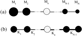
Figure 1: /Xiao, Yakubo, and Yu

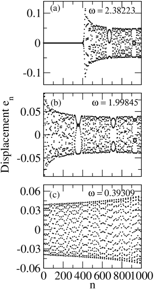
Figure 4: /Xiao, Yakubo, and Yu

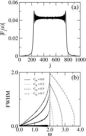
Figure 5: /Xiao, Yakubo, and Yu