Zitterbewegung of electrons and holes in III-V semiconductor quantum wells

Abstract

The notion of zitterbewegung is a long-standing prediction of relativistic quantum mechanics. Here we extend earlier theoretical studies on this phenomenon for the case of III-V zinc-blende semiconductors which exhibit particularly strong spin-orbit coupling. This property makes nanostructures made of these materials very favorable systems for possible experimental observations of zitterbewegung. Our investigations include electrons in n-doped quantum wells under the influence of both Rashba and Dresselhaus spin-orbit interaction, and also the two-dimensional hole gas. Moreover, we give a detailed anaysis of electron zitterbewegung in quantum wires which appear to be particularly suited for experimentally observing this effect.

]

I introduction

The spin degree of freedom of electrons in semiconductor nanostructures is one of the central subjects in the growing field of spin electronics overview . The latter key word describes the whole variety of efforts and proposals for using the electron spin instead, or in combination with, its charge for information processing, or, even more ambitious, quantum information processing. A central issue is the possibility of electrical control electron spins, which avoids many difficulties arising from applying and gating magnetic fields. Zinc-blende III-V semiconductors show a particularly strong spin-orbit interaction and are therefore natural candidates with respect to the above goals.

In the present paper we extend earlier results on the relativistic effect of zitterbewegung in systems of the above type Schliemann05a . In this context we also discuss related recent work by other authors Jiang05 ; Zawadzki05a ; Lee05 ; Nikolic05 ; Shen05 ; Zawadzki05b . Our investigations include electrons in n-doped quantum wells under the influence of both Rashba and Dresselhaus spin-orbit interaction, and holes in two-dimensional geometry. Phenomena related to spin-orbit coupling in such systems are presently studied very intensively also in the context of the intrinsic spin-Hall effect Murakami03 ; Sinova04 ; Schliemann05b . Particular attention is paid to the case of electron zitterbewegung in quantum wires which appear to be good candidates for experimental investigations of this effect.

The coupling between the orbital and the spin degree of freedom of electrons is a relativistic effect described by the Dirac equation and its nonrelativistic expansion in powers of the inverse speed of light $c$ Feshbach58 . In second order one obtains, apart from two spin-independent contributions, the following well-known spin-orbit coupling term,

$${\cal H}_{so}=\frac{1}{2m_{0}c^{2}}\vec{s}\cdot\left(\nabla V\times\frac{\vec{p}}{m_{0}}\right)\,,$$ (1)

where $m_{0}$ is the bare mass of the electron, $\vec{s}$, $\vec{p}$ its spin and momentum, respectively, and $V$ is some applied external potential. On the other hand, the free Dirac equation, $V=0$, has two dispersion branches with positive and negative energy,

$$\varepsilon(\vec{p})=\pm\sqrt{m_{0}^{2}c^{4}+c^{2}p^{2}}\,,$$ (2)

which are separated by an energy gap of $2m_{0}c^{2}\approx 1{\rm MeV}$. In particular, the nonrelativistic expansion of the Dirac equation quoted above can be seen as a method of systematically including the effects of the negative-energy solutions on the states of positive energy starting from their nonrelativistic limit Feshbach58 . Moreover, the large energy gap $2m_{0}c^{2}$ appears in the denominator of the right hand side of Eq. (1), suppressing the effects of spin-orbit coupling for weakly bound electrons.

On the other hand, the band structure of zinc-blende III-V semiconductors shows many formal similarities to the situation of free relativistic electrons, while the relevant energy scales are grossly different Zawadzki70 ; Darnhofer93 ; Rashba04 . For not too large doping of such semiconductors, one can concentrate on the band structure around the $\Gamma$ point. Here one has a parabolic $s$-type conduction band and a $p$-type valence band consisting of the well-known dispersion branches for heavy and light holes, and the split-off band. However, the gap between conduction and valence band is of order $1{\rm eV}$ or smaller. This heuristic argument makes plausible that spin-orbit coupling is an important effect in III-V semiconductors which actually lies at the very heart of the field of semiconductor spintronics.

Dating back to a seminal paper by Schrödinger Schrodinger30 ; Barut81 from 1930, the notion of zitterbewegung has been a long-standing theoretical prediction of relativistic quantum mechanics. In the free Dirac equation, this oscillatory quantum motion occurs for particle wave packets which are superpositions of both solutions of positive and negative energy. Thus, the dominant frequency of this dynamics is given by $2m_{0}c^{2}/{\hbar}$ which is of order $10^{20}{\rm Hz}$. Moreover, the length scale of this motion is given by the Compton wave length $\hbar/m_{0}c$ of the free electron. Therefore, in order to experimentally observe the zitterbewegung of free electrons one would need to confine these objects on a length scale of a few picometers. Now it follows form general uncertainty arguments that such a spatial confinement leads to an energy scale where electron-positron pair production plays a serious and detrimental role. These arguments have led many authors to the opinion that the zitterbewegung of electrons is impossible to observe, see e.g. Ref. Huang52 .

Most recently, we have theoretically investigated zitterbewegung in III-V zinc-blende semiconductors and developed a proposal for its experimental observation. As already mentioned, the mathematical treatment of effective band structure models relevant to such systems on the one hand, and the nonrelativistic expansion of the Dirac equation on the other hand show many formal similarities Zawadzki70 ; Darnhofer93 ; Rashba04 . In fact, under certain aspects, the low-energy band structure of such semiconductors around the Fermi level can be viewed as a model for truly relativistic electrons, but with energy and length scales which are much more favourable for observing effects like zitterbewegung.

This paper is organized as follows. In section II we study zitterbewegung in the two-dimensional electron gas. We extend previous results Schliemann05a to the situation where spin-orbit coupling of both the Rashba and Dresselhaus type is present. Moreover, we give a deeper discussion of zitterbewegung in quantum wires and our related experimental proposal. Section III is devoted to the same phenomenon for heavy holes in two-dimensional quantum wells. We close with conclusions in section IV.

II Zitterbewegung in the two-dimensional electron gas and in quantum wires

II.1 The two-dimensional electron gas

For conduction band electrons in $n$-doped quantum wells of zinc-blende semiconductor structures the dominant effects of spin-orbit interaction can be described in terms of two effective contributions to the Hamiltonian. On of them is the Rashba spin-orbit term Rashba60 which is due to the inversion-asymmetry of the confining potential and has the form

$${\cal H}_{R}=\frac{\alpha}{\hbar}\left(p_{x}\sigma^{y}-p_{y}\sigma^{x}\right)\,,$$ (3)

where $\vec{p}$ is the momentum of the electron confined in a two-dimensional geometry, and $\vec{\sigma}$ the vector of Pauli matrices. The coefficient $\alpha$ is tunable in strength by the external gate perpendicular to the plane of the two-dimensional electron gas. The other contribution is the Dresselhaus spin-orbit term which is present in semiconductors lacking bulk inversion symmetryDresselhaus55 . When restricted to a two-dimensional semiconductor nanostructure grown along the $[001]$ direction this coupling is of the form Dyakonov86 ; Bastard92

$${\cal H}_{D}=\frac{\beta}{\hbar}\left(p_{y}\sigma^{y}-p_{x}\sigma^{x}\right)\,,$$ (4)

where the coefficient $\beta$ is determined by the semiconductor material and the geometry of the sample. These two contributions to the effective Hamiltonian have also an interesting interplay Schliemann03a ; Schliemann03b .

We now consider the single-particle Hamiltonian of a free electron under the influence of spin-orbit coupling of both the Rashba and the Dresselhaus type,

$${\cal H}=\frac{\vec{p}^{2}}{2m}+{\cal H}_{R}+{\cal H}_{D}\,,$$ (5)

where $m$ is the effective band mass. The components of the time-dependent position operator

$$\vec{r}_{H}(t)=e^{i{\cal H}t/\hbar}\vec{r}(0)e^{-i{\cal H}t/\hbar}$$ (6)

in the Heisenberg picture read explicitly

$$x_{H}(t) = x(0)+\frac{p_{x}}{m}t+\left(\frac{\alpha}{\hbar}\sigma^{y}-\frac{\beta}{\hbar}\sigma^{x}\right)t$$ (7)

$$+ \frac{\alpha^{2}-\beta^{2}}{\Lambda^{2}}p_{y}\left(1-\cos\left(\frac{2}{\hbar^{2}}\Lambda t\right)\right)\frac{\hbar}{2}\sigma^{z}$$

$$+ \frac{\alpha^{2}-\beta^{2}}{\Lambda^{3}}p_{y}\left(\frac{2}{\hbar^{2}}\Lambda t-\sin\left(\frac{2}{\hbar^{2}}\Lambda t\right)\right)\Sigma\,,$$

$$y_{H}(t) = x(0)+\frac{p_{y}}{m}t-\left(\frac{\alpha}{\hbar}\sigma^{x}-\frac{\beta}{\hbar}\sigma^{y}\right)t$$ (8)

$$- \frac{\alpha^{2}-\beta^{2}}{\Lambda^{2}}p_{x}\left(1-\cos\left(\frac{2}{\hbar^{2}}\Lambda t\right)\right)\frac{\hbar}{2}\sigma^{z}$$

$$- \frac{\alpha^{2}-\beta^{2}}{\Lambda^{3}}p_{x}\left(\frac{2}{\hbar^{2}}\Lambda t-\sin\left(\frac{2}{\hbar^{2}}\Lambda t\right)\right)\Sigma$$

with

$$\Lambda^{2}(\vec{p};\alpha,\beta)=\left(\alpha^{2}+\beta^{2}\right)p^{2}+4\alpha\beta p_{x}p_{y}$$ (9)

and

$$\Sigma(\vec{p},\vec{\sigma};\alpha,\beta) = \frac{\hbar}{2}\Bigl{(}\alpha\left(p_{x}\sigma^{x}+p_{y}\sigma^{y}\right)$$ (10)

$$+\beta\left(p_{x}\sigma^{y}+p_{y}\sigma^{x}\right)\Bigr{)}\,.$$

Here the operators $\vec{p}$ and $\vec{\sigma}$ on the right hand sides are in the Schrödinger picture and therefore time-independent.

The oscillatory terms on the right hand sides of Eqs. (7), (8) can be viewed as the zitterbewegung the electron performs under the influence of spin-orbit coupling. This oscillatory quantum motion vanishes if relativistic effects are absent, $\alpha=\beta=0$. The contributions linear in time $t$ in the first lines in Eqs. (7),(8) are just proportional to the velocity

$$\vec{v}=\frac{i}{\hbar}\left[{\cal H},\vec{r}\right]\,,$$ (11)

which is in the presence of spin-orbit coupling a spin-dependent operator. The expressions (7),(8) contain the results given in Ref. Schliemann05a for pure Rashba or Dresselhaus coupling as special cases. For, instance, if only Rashba coupling is present $(\beta=0)$, one can express the position operator in the Heisenberg picture as

$$x_{H}(t) = x(0)+\frac{p_{x}}{m}t+\frac{p_{y}}{p^{2}}\frac{\hbar}{2}\sigma^{z}\left(1-\cos\left(\frac{2\alpha p}{\hbar^{2}}t\right)\right)$$ (12)

$$+ \frac{p_{x}}{p^{3}}\frac{\hbar}{2}\left(p_{x}\sigma^{y}-p_{y}\sigma^{x}\right)\left(\frac{2\alpha p}{\hbar^{2}}t-\sin\left(\frac{2\alpha p}{\hbar^{2}}t\right)\right)$$

$$+ \frac{1}{p}\frac{\hbar}{2}\sigma^{y}\sin\left(\frac{2\alpha p}{\hbar^{2}}t\right)\,,$$

$$y_{H}(t) = y(0)+\frac{p_{y}}{m}t-\frac{p_{x}}{p^{2}}\frac{\hbar}{2}\sigma^{z}\left(1-\cos\left(\frac{2\alpha p}{\hbar^{2}}t\right)\right)$$ (13)

$$+ \frac{p_{y}}{p^{3}}\frac{\hbar}{2}\left(p_{x}\sigma^{y}-p_{y}\sigma^{x}\right)\left(\frac{2\alpha p}{\hbar^{2}}t-\sin\left(\frac{2\alpha p}{\hbar^{2}}t\right)\right)$$

$$- \frac{1}{p}\frac{\hbar}{2}\sigma^{x}\sin\left(\frac{2\alpha p}{\hbar^{2}}t\right)\,.$$

The case $\alpha=\pm\beta$ is particular Schliemann03a ; Schliemann03b . As seen from Eqs. (7),(8), the oscillatory part of the time-dependent position operator, i.e. the zitterbewegung vanishes due to the prefactor $(\alpha^{2}-\beta^{2})$. Physically, this observation results from an additional conserved quantity arising at this point Schliemann03a ; Schliemann03b .

It is straightforward to evaluate the above time-dependent position operators within Gaussian wave packets. For simplicity we concentrate on the case of pure Rashba coupling described by Eqs (12),(13). We consider a Gaussian wave packet with initial spin polarization along the $z$-direction perpendicular to the quantum well,

$$\langle\vec{r}|\psi\rangle=\frac{1}{2\pi}\frac{d}{\sqrt{\pi}}\int d^{2}k\,e^{-\frac{1}{2}d^{2}\left(\vec{k}-\vec{k}_{0}\right)^{2}}e^{i\vec{k}\vec{r}}\left(\begin{array}[]{c}1\\ 0\end{array}\right)\,.$$ (14)

Clearly we have $\langle\psi|\vec{r}|\psi\rangle=0$, $\langle\psi|\vec{p}|\psi\rangle=\hbar\vec{k}_{0}$, and the variances of the position and momentum operators are $\left(\Delta x\right)^{2}=\left(\Delta y\right)^{2}=d^{2}/2$, $\left(\Delta p_{x}\right)^{2}=\left(\Delta p_{y}\right)^{2}=\hbar^{2}/2d^{2}$. Thus, the group velocity of the wave packet is given by $\hbar\vec{k}_{0}/m$ , while its spatial width is described by the parameter $d$ with the minimum uncertainty product typical for Gaussian wave packets, $\Delta p_{x}\Delta x=\Delta p_{y}\Delta y=\hbar/2$.

A direct calculation gives

$$\langle\psi|x_{H}(t)|\psi\rangle = \frac{\hbar k_{0x}}{m}+\frac{d}{2\pi}e^{-d^{2}k_{0}^{2}}\int_{0}^{2\pi}d\varphi\sin\varphi$$ (15)

$$\cdot\int_{0}^{\infty}dq\,e^{-q^{2}+2dq\left(k_{0x}\cos\varphi+k_{0y}\sin\varphi\right)}$$

$$\qquad\cdot\left(1-\cos\left(\frac{2\alpha q}{\hbar d}t\right)\right)\,.$$

In the above expression $q$ is a dimensionless integration variable. The remaining integration over the polar angle $\varphi$ gives a vanishing result if $k_{0y}=0$, i.e. if the group velocity is along the $x$-direction. More generally, one finds that

$$\langle\psi|\vec{k}_{0}\cdot\vec{r}_{H}(t)/k_{0}|\psi\rangle=\frac{\hbar k_{0}}{m}t\,,$$ (16)

which means that the zitterbewegung is always perpendicular to the group velocity of the wave packet. The same observation is made for the case of pure Dresselhaus coupling, $\alpha=0$. Note that for pure Rashba coupling the sum of the $z$-component of the orbital angular momentum $\vec{l}=\vec{r}\times\vec{p}$ and the $z$-component of the spin $\vec{s}=\hbar\vec{\sigma}/2$ is a conserved quantity, $[{\cal H},l^{z}+s^{z}]=0$, while for pure Dresselhaus coupling we have $[{\cal H},l^{z}-s^{z}]=0$. In the presence of these conservation laws, the zitterbewegung can also be interpreted as a consequence of spin rotation due to spin-orbit coupling. Consider for instance an electron moving along the $y$-direction with its spin being initially aligned with the $z$-direction. In the time evolution of the particle, the spin will then be rotated due spin-orbit coupling which requires, by virtue of the conservation law, also a finite component $l^{z}$ to develop, i.e. the electron has to perform also a movement perpendicular to its group velocity. In the general case $\alpha\neq 0\neq\beta$ such an interpretation does not seem to be possible since a conserved quantity of the above kind does not exist.

Let us turn back to the case of pure Rashba coupling. Without loss of generality we consider an electron wave packet moving along the $y$-direction, $k_{0x}=0$. By expanding the exponential containing the trigonometric functions in Eq. (15), one derives noteerratum

$$\langle\psi|x_{H}(t)|\psi\rangle = \frac{1}{2k_{0y}}\left(1-e^{-d^{2}k_{0y}^{2}}\right)$$ (17)

$$- \frac{1}{k_{0y}}e^{-d^{2}k_{0y}^{2}}\sum_{n=0}^{\infty}\Biggl{[}\frac{\left(dk_{0y}\right)^{2(n+1)}}{n!(n+1)!}$$

$$\cdot\int_{0}^{\infty}dqq^{2n+1}e^{-q^{2}}\cos\left(\frac{2\alpha q}{\hbar d}t\right)\Biggr{]}\,.$$

Thus, the amplitude of the zitterbewegung is proportional to the wave length $\lambda_{0y}=2\pi/k_{0y}$ of the electron motion perpendicular to it. In a semiconductor quantum well, this length can be of order a few ten nanometers, which is several orders of magnitude larger than the length scale of the zitterbewegung of free electrons given by the Compton wave length. Note also that the oscillatory zitterbewegung changes its sign if the translational motion is reversed.

If the product $dk_{0y}$ is not too large, $dk_{0y}\lesssim 1$, only low values of the summation index $n$ in Eq. (17) lead to substantial contributions, and the Gaussian factor in the integrand suppresses contributions from large values of $q$. Thus, a typical scale of this integration variable is leading to sizable contributions is $q\approx 1/\sqrt{2}$. Thus, a typical time scale in the integrand is $T=\sqrt{2}\pi\hbar d/\alpha$, and when averaging the zitterbewegung over times scales significantly larger than $T$, the cosine term drops giving

$$\overline{\langle\psi|x_{H}(t)|\psi\rangle}=\frac{1}{2k_{0y}}\left(1-e^{-d^{2}k_{0y}^{2}}\right)\,,$$ (18)

i.e. the time-averaged guiding center of the wave packet is shifted perpendicular to its direction of motion. Note that the zitterbewegung is absent for $k_{0y}=0$ Huang52 .

In the opposite case $dk_{0y}\gg 1$ the Gaussian approaches a $\delta$-function. In this limit one finds (for $k_{0x}=0$)

$$\langle\psi|x_{H}(t)|\psi\rangle=\frac{1}{2k_{0y}}\left(1-\cos\left(\frac{2\alpha k_{0y}}{\hbar}t\right)\right)\,.$$ (19)

Here the frequency of the zitterbewegung is $\Omega=2\alpha k_{0y}/\hbar$, and the guiding center of the wave packet is also shifted in the direction perpendicular to its group velocity. Note that $\hbar\Omega$ is the excitation energy between the two branches of the Rashba Hamiltonian ${\cal H}$ at a given momentum $\vec{k}=k_{0y}\vec{e}_{y}$. Rashba spin-orbit coupling is particularly strong in InAs where values for the parameter $\alpha$ of a few $10^{-11}{\rm eVm}$ can be reached Nitta97 ; Engels97 ; Heida98 ; Hu99 ; Grundler00 ; Sato01 ; Hu03 , leading to frequencies $\Omega$ is the terahertz regime. This is much smaller than the typical frequency of the zitterbewegung of free electrons which is of order $10^{20}{\rm Hz}$. For GaAs, the Rashba coefficient is typically an order of magnitude smaller than in InAs Miller03 and the Dresselhaus coupling plays a more important role Lommer88 ; Jusserand92 ; Jusserand95 . In summary, the zitterbewegung of electronic wave packets in semiconductor quantum wells as discussed above is characterized by amplitudes and frequencies which are by orders of magnitude larger and smaller, respectively, than it is the case for free electrons. This opens the perspective to experimentally observe the electron zitterbewegung in semiconductor nanostructures via terahertz methods, or using high-resolution scanning-probe microscopy imaging techniques as developed and discussed in Refs. Topinka00 ; LeRoy03 . The latter approach will be described in more detail in section II.2.

The issue of zitterbewegung of electrons in III-V semiconductors was also discussed recently by Zawadzki where the three-dimensional bulk case was considered Zawadzki05a . The author starts from an $8\times 8$ Kane model for conduction and valence band being diagonal in the hole sector Darnhofer93 ; Vurgaftman01 . Specializing on particles moving along the $z$-direction in real space and neglecting the split-off band, the author obtains an effective Hamiltonian coupling only light holes and conduction band electron states. Moreover, for an appropriate choice of basis this Hamiltonian matrix mimics the Hamiltonian of the free Dirac equation, which enables to derive a zitterbewegung following directly Schrödinger’s original approach Schrodinger30 ; Barut81 . However, when reducing the underlying $8\times 8$ Kane model in a systematic way to an effective $2\times 2$ Hamiltonian for conduction band electrons only, one obtains in the absence of an additional potential and magnetic fields to second order in the gap energy only a kinetic term involving an effective mass depending on band structure parameters Darnhofer93 . This is analogous to the situation of the free Dirac equation where, again in the absence of external fields, the lowest-order relativistic correction is an additional contribution to the kinetic energy which does not lead to zitterbewegung Feshbach58 . The zitterbewegung studied in the present work occurs, for the case of Rashba coupling, due to an external potential introducing structure-inversion asymmetry Rashba60 ; Darnhofer93 . For the case of Dresselhaus coupling, it stems from the bulk Dresselhaus coupling term which results from bulk-inversion asymmetry Dresselhaus55 and is not included in the $8\times 8$ Kane model. In this sense, Zawadzki’s result appears to be effect of higher order in the inverse gap energy which can be of importance in materials with particularly small gap such as InSb Vurgaftman01 . Moreover, the zitterbewegung as discussed in Ref. Zawadzki05a occurs always in in the direction of the group velocity of the particle wave packet, i.e. in the $z$-direction. This feature is clearly different from the zitterbewegung investigated here and might pose an obstacle against experimentally observing this effect.

II.2 Quantum wires

The zitterbewegung of an electron in a quantum well as described above is naturally accompanied by a broadening of the wave packet, where the dominant contribution stems from the dispersive effective-mass term in the Hamiltonian. Such a broadening might pose an obstacle for experimentally detecting the zitterbewegung. However, the broadening can be efficiently suppressed and limited if the electron moves along a quantum wire. In fact, the motion of electrons in quantum wells is generally under better control if additional lateral confinement is present. We therefore consider a harmonic quantum wire along the $y$-direction described by

$${\cal H}=\frac{\vec{p}^{2}}{2m}+\frac{1}{2}m\omega^{2}x^{2}+{\cal H}_{R}\,,$$ (20)

where the frequency $\omega$ parameterizes the confining potential perpendicular to the wire wire ; Governale02 . It is instructive to write the Hamiltonian in the form

$${\cal H}={\cal H}_{0}+{\cal H}_{1}$$ (21)

with

$${\cal H}_{0} = \hbar\omega\left(a^{+}a+\frac{1}{2}\right)+\frac{\hbar^{2}k_{0y}^{2}}{2m}+\alpha k_{0y}\sigma^{x}\,,$$ (22)

$${\cal H}_{1} = -i\sqrt{\frac{\hbar m\omega}{2}}\frac{\alpha}{\hbar}\left(a-a^{+}\right)\sigma^{y}\,.$$ (23)

Here $a$, $a^{+}$ are the usual harmonic climbing operators, and $k_{0y}$ is the component of the electron wave vector along the quantum wire. Due to the properties of the “mixing operator” ${\cal H}_{1}$, analytical progress as before without employing further approximations does not seem to be possible. We therefore project the Hamiltonian ${\cal H}$ onto the lowest two orbital subbands. This approximation is known to give very reasonable results for not too wide quantum wells Governale02 , and we will also compare its results with a full numerical simulation of the above multi-band Hamiltonian.

For a given $k_{0y}$ the truncated Hilbert space is spanned by the states $|0,\uparrow\rangle$, $|0,\downarrow\rangle$, $|1,\uparrow\rangle$, $|1,\downarrow\rangle$, where the arrows denote the spin state with respect to the $z$-direction, and $0$ and $1$ stand for the ground state and the first excited state of the harmonic potential, respectively. In the above basis, the truncated Hamiltonian reads

$${\cal H}=\left(\begin{array}[]{cccc}\varepsilon_{0}&-\alpha k_{0y}&0&-\sqrt{\frac{\hbar\omega\varepsilon_{R}}{2}}\\ -\alpha k_{0y}&\varepsilon_{0}&\sqrt{\frac{\hbar\omega\varepsilon_{R}}{2}}&0\\ 0&\sqrt{\frac{\hbar\omega\varepsilon_{R}}{2}}&\varepsilon_{1}&-\alpha k_{0y}\\ -\sqrt{\frac{\hbar\omega\varepsilon_{R}}{2}}&0&-\alpha k_{0y}&\varepsilon_{1}\end{array}\right)$$ (24)

with

$$\varepsilon_{0} = \frac{1}{2}\hbar\omega+\frac{\hbar^{2}k_{0y}^{2}}{2m}\,,$$ (25)

$$\varepsilon_{1} = \frac{3}{2}\hbar\omega+\frac{\hbar^{2}k_{0y}^{2}}{2m}$$ (26)

being the subband energies in the absence of spin-orbit coupling, and $\varepsilon_{R}=m\alpha^{2}/\hbar^{2}$ is the energy scale of the Rashba coupling. When applying the transformation

$$U=\frac{1}{\sqrt{2}}\left(\begin{array}[]{cccc}1&1&0&0\\ 0&0&1&-1\\ 1&-1&0&0\\ 0&0&1&1\end{array}\right)$$ (27)

the projected Hamiltonian and in turn the time evolution operator become block-diagonal,

$$Ue^{-\frac{i}{\hbar}Ht}U^{+}=\left(\begin{array}[]{cc}h_{+}(t)&0\\ 0&h_{-}(t)\end{array}\right)$$ (28)

where

$$h_{\pm}(t) = \left({\bf 1}\cos\left(\frac{1}{\hbar}\mu_{\pm}t\right)-i\frac{\vec{\mu}_{\pm}}{\mu_{\pm}}\cdot\vec{\sigma}\sin\left(\frac{1}{\hbar}\mu_{\pm}t\right)\right)$$ (29)

$$\cdot\exp\left(-\frac{i}{\hbar}\left(\hbar\omega+\frac{\hbar^{2}k_{0y}^{2}}{2m}\right)t\right)$$

and

$$\vec{\mu}_{\pm}=\left(\pm\alpha\sqrt{\frac{m\omega}{2\hbar}},0,-\frac{\hbar\omega}{2}\mp\alpha k_{0y}\right)\,.$$ (30)

Let us first consider an electron with a given momentum $k_{0y}$ along the wire and injected initially into the lowest subband of the confining potential with the spin pointing upwards along the $z$-direction, i.e. the initial wave function $|\psi_{z}\rangle=|0,\uparrow\rangle$ for the $x$-direction is a Gaussian whose width is determined by the characteristic length $\lambda=\sqrt{\hbar/m\omega}$ of the harmonic confinement. Using

$$UxU^{+}=\frac{\lambda}{\sqrt{2}}\left(\begin{array}[]{cc}0&\sigma^{x}\\ \sigma^{x}&0\end{array}\right)$$ (31)

one obtains for the above initial state the following time-dependent expectation value

$$\langle\psi_{z}|x_{H}(t)|\psi_{z}\rangle = \frac{\lambda}{\sqrt{2}}\frac{\mu_{+}^{x}\mu_{-}^{z}+\mu_{-}^{x}\mu_{+}^{z}}{\mu_{+}\mu_{-}}$$ (32)

$$\cdot\sin\left(\frac{1}{\hbar}\mu_{+}t\right)\sin\left(\frac{1}{\hbar}\mu_{-}t\right)\,.$$

The amplitude of this oscillatory dynamics perpendicular to the wire direction becomes maximal when the resonance condition $\hbar\omega=\pm 2\alpha k_{0y}$ is fulfilled. At that point we have $\mu_{\mp}^{z}=0$, and if $\mu_{\pm}^{x}$ can be neglected compared to $\mu_{\pm}^{z}$ (which is the case for large enough $k_{0y}$) the amplitude of the zitterbewegung is approximately $\lambda/\sqrt{2}$. This result from the truncated Hamiltonian is in excellent agreement with numerical simulations of the full multi-band system. In Fig. 1 we have plotted simulation results for $\langle\psi_{z}|x_{H}(t)|\psi_{z}\rangle$ where the wave number along the wire is fixed to be $k_{0y}\lambda=5$ and the Rashba parameter $\alpha$ is varied around the resonance condition. Clearly, the amplitude is maximum at resonance.Equivalent observation are made if the Rashba coupling is fixed while the wave number $k_{0y}$ is varied. In Fig. 2 we have plotted the amplitude of the zitterbewegung as a function of $\Omega/\omega=2\alpha k_{0y}/\hbar\omega$ for different values of the wave number $k_{0y}$ along the wire. In this range of parameters, the resonance becomes narrower with increasing $k_{0y}$, while its maximum value is rather independent of this quantity and remarkably well described by $\lambda/\sqrt{2}$.

A qualitative explanation for this resonance can be given in terms of the decomposition ${\cal H}={\cal H}_{0}+{\cal H}_{1}$ of the Hamiltonian. The zitterbewegung is induced by the perturbation ${\cal H}_{1}$ which can act most efficiently if the unperturbed energy levels of ${\cal H}_{0}$ are degenerate having opposite spins. This is the case at $|2\alpha k_{0y}|=\hbar\omega$.

We propose that electron zitterbewegung in semiconductor nanostructures as described above can be experimentally observed using high-resolution scanning-probe microscopy imaging techniques as developed and discussed in Refs. Topinka00 ; LeRoy03 . As a possible setup, a tip can be moved along the wire and centered in its middle. For an appropriate biasing of the tip, the electron density at its location is partially depleted leading to a reduced conductance of the wire. Since the amplitude of the zitterbewegung reflects the electron density in the center of the wire, the zitterbewegung will induce beatings in the wire conductance as a function of the tip position. These beatings are most pronounced at the resonance, see Fig. 1. Note that the oscillations shown there as a function of time can be easily converted to the real-space $y$-coordinate by multiplying the abscissa by $\hbar k_{0y}/m$. Moreover, for tuning the system to the resonance condition $|2\alpha k_{0y}|=\hbar\omega$, at least two parameters can be varied expertimentally: The group velocity of the injected electron along the wire given by $k_{0y}$, and the Rashba parameter $\alpha$ which is tunable by a gate voltage across the quantum well. Thus, quantum wires defined in InAs quantum wells are favorable systems for experiments of the above kind, since this material can exhibit a quite large Rashba coupling but has a comparatively small Dresselhaus term. The group velocity can be varied by changing the gate to the two-dimensional electron gas. This alters the global electron density and therefore also the wave vector for motion along the wire. Generally we expect spin-orbit effects in STM experiments to be more pronounced in the presence of additional confinement such as in a quantum wire.

The present considerations concentrate on the case of pure Rashba coupling neglecting a possible Dresselhaus contribution. Very analogous observations as above can be made for pure Dresselhaus coupling, while in the case of both couplings being present the analytical theory becomes technically more involved. We note that the Dresselhaus coupling, differently from the Rashba term, cannot be tuned by an external gate. Therefore, materials with pronounced Rashba coupling are favorable for tuning the system to the above resonance condition.

Let us now analyze the situation when the electron is injected into the lowest subband of the wire, but its spin is not aligned with the $z$-direction. If the spin points along the $x$-direction, no zitterbewegung occurs,

$$\langle\psi_{x}|x_{H}(t)|\psi_{x}\rangle=0\,.$$ (33)

This is a property of both the full multi-band model and the truncated Hamiltonian and follows from symmetry considerations: Under a reflection in the $yz$-plane $x$, $p_{x}$ and the $y$- and $z$-component of the spin change sign while the other components of spin and momentum remain unchanged. Thus, the Hamiltonian is invariant under this operation, a property which is also shared by the initial state $|\psi_{x}\rangle$. Therefore, the expectation value of $x_{H}(t)$ has to be equal to its negative and is consequently zero. Finally, if the spin points initially along the $y$-direction one finds from the truncated Hamiltonian

$$\langle\psi_{y}|x_{H}(t)|\psi_{y}\rangle = \frac{\lambda}{\sqrt{2}}\frac{1}{2}\Biggl{[}\frac{\mu_{+}^{x}\mu_{-}^{z}+\mu_{-}^{x}\mu_{+}^{z}}{\mu_{+}\mu_{-}}$$ (34)

$$\cdot\sin\left(\frac{1}{\hbar}\mu_{+}t\right)\sin\left(\frac{1}{\hbar}\mu_{-}t\right)$$

$$+ \frac{\mu_{+}^{x}}{\mu_{+}}\cos\left(\frac{1}{\hbar}\mu_{+}t\right)\sin\left(\frac{1}{\hbar}\mu_{-}t\right)$$

$$- \frac{\mu_{-}^{x}}{\mu_{-}}\sin\left(\frac{1}{\hbar}\mu_{+}t\right)\cos\left(\frac{1}{\hbar}\mu_{-}t\right)\Biggr{]}\,.$$

Thus, the zitterbewegung also occurs if the electron spin is initially aligned along the wire direction.

It is instructive to also investigate the dynamics of the spin degree of freedom as the electron passes along the wire. For a situation where the spin is pointing again initially in the $z$-direction, the truncated Hamiltonian leads to the following expressions:

$$\langle\psi_{z}|\sigma^{x}_{H}(t)|\psi_{z}\rangle=\frac{1}{2}\Biggl{[}\cos^{2}\left(\frac{1}{\hbar}\mu_{+}t\right)$$

$$\qquad+\frac{-\left(\mu_{+}^{x}\right)^{2}+\left(\mu_{+}^{z}\right)^{2}}{\mu_{+}^{2}}\sin^{2}\left(\frac{1}{\hbar}\mu_{+}t\right)$$

$$\qquad-\cos^{2}\left(\frac{1}{\hbar}\mu_{-}t\right)$$

$$\qquad-\frac{-\left(\mu_{-}^{x}\right)^{2}+\left(\mu_{-}^{z}\right)^{2}}{\mu_{-}^{2}}\sin^{2}\left(\frac{1}{\hbar}\mu_{-}t\right)\Biggr{]}\,,$$ (35)

$$\langle\psi_{z}|\sigma^{y}_{H}(t)|\psi_{z}\rangle = \frac{\mu_{-}^{z}}{\mu_{-}}\cos\left(\frac{1}{\hbar}\mu_{+}t\right)\sin\left(\frac{1}{\hbar}\mu_{-}t\right)$$ (36)

$$+ \frac{\mu_{+}^{z}}{\mu_{+}}\cos\left(\frac{1}{\hbar}\mu_{-}t\right)\sin\left(\frac{1}{\hbar}\mu_{+}t\right)\,,$$

$$\langle\psi_{z}|\sigma^{z}_{H}(t)|\psi_{z}\rangle = \cos\left(\frac{1}{\hbar}\mu_{+}t\right)\cos\left(\frac{1}{\hbar}\mu_{-}t\right)$$ (37)

$$+ \frac{\mu_{+}^{x}\mu_{-}^{x}+\mu_{+}^{z}\mu_{-}^{z}}{\mu_{+}\mu_{-}}$$

$$\cdot\sin\left(\frac{1}{\hbar}\mu_{+}t\right)\sin\left(\frac{1}{\hbar}\mu_{-}t\right)\,.$$

Interestingly the expectation value $\langle\psi_{z}|\sigma^{x}_{H}(t)|\psi_{z}\rangle$ shows a particular behavior at the resonance $\hbar\omega=\pm 2\alpha k_{0y}$. Here we have $\mu_{\mp}^{z}=0$, and if $\mu_{\pm}^{x}$ can again be neglected compared to $\mu_{\pm}^{z}$ (as it is the case for the choice of parameters used in Figs. 1,2), this expectation value is approximately given by

$$\langle\psi_{z}|\sigma^{x}_{H}(t)|\psi_{z}\rangle\approx\pm\left(1-\cos\left(\frac{2}{\hbar}\mu^{x}_{\mp}t\right)\right)\,.$$ (38)

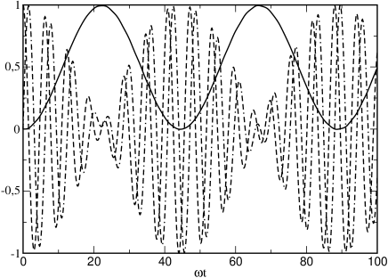
Figure 3: The spin expectation values $\langle\psi_{z}|\vec{\sigma}_{H}(t)|\psi_{z}\rangle$ as a function of time at the resonance condition $2\alpha k_{0y}=\hbar\omega$ with $k_{0y}\lambda=5$ (cf. mid panel of Fig. 1). The time evolution of $\langle\psi_{z}|\sigma^{x}_{H}(t)|\psi_{z}\rangle$ (solid line) is governed by a single frequency as shown in Eq. (38), while the other components $\langle\psi_{z}|\sigma^{y}_{H}(t)|\psi_{z}\rangle$ and $\langle\psi_{z}|\sigma^{z}_{H}(t)|\psi_{z}\rangle$ (dashed lines) show beatings between two frequencies given by $\mu_{\pm}$.

Thus, the time dependence is, to a very good degree of approximation, governed by a single frequency. This remarkable result is also confirmed by numerical simulations of the full multiband model shown in Fig. 3.

Finally, if the electron spin points initially in the $x$-direction, we have

$$\langle\psi_{x}|\sigma^{x}_{H}(t)|\psi_{x}\rangle = \cos^{2}\left(\frac{1}{\hbar}\mu_{+}t\right)$$ (39)

$$+ \frac{-\left(\mu_{+}^{x}\right)^{2}+\left(\mu_{+}^{z}\right)^{2}}{\mu_{+}^{2}}\sin^{2}\left(\frac{1}{\hbar}\mu_{+}t\right)$$

while the expectation values of the other two spin components strictly vanish. The latter result is also true for the full multi-band model and follows from the same symmetry considerations as above.

Let us finally summarize other recent theoretical developments pertaining to the issue of zitterbewegung in quantum wires. The electron dynamics in ballistic quantum wires in the presence of spin-orbit coupling were also recently analyzed by Nikolic, Zarba, and Welack concentrating on transverse forces on the electron induced by spin-orbit coupling Nikolic05 . A study similar in spirit was carried out by Shen, who also made a connection between transverse forces due to spin-orbit interaction and the occurrence of zitterbewegung Shen05 . Lee and Bruder studied recently quantum wires with spin-orbit coupling of both the Rashba and Dresselhaus type Lee05 . Their approach is mainly numerical and concentrates on mapping out charge- and spin-density modulations in ferromagnet-semiconductor single-junction quantum wires. The shape of these modulations is explained in terms of the symmetry properties of the eigenstates of the wire. Finally, Zawadzki has most recently analysed the band structure of narrow-gap single-wall carbon nanotubes making a connections to relativistic effects in the free Dirac equation Zawadzki05b . Similarly to Ref. Zawadzki05a , the kind of zitterbewegung predicted from these investigations is along the group velocity of the electron wave packet, i.e. along the wire, which is considered there as a strictly one-dimensional system. This is in contrast to the present study where we consider a quantum wire of finite width and obtain a zitterbewegung of electronic wave packets perpendicular to the wire direction.

III Holes in a two-dimensional quantum well

We now turn to the case of holes in the p-type valence band of III-V semiconductors as opposed to s-type conduction band electrons studied so far. We note that Jiang et al. have very recently performed a semiclassical study of the time evolution of holes in three-dimensional bulk systems under the influence of a homogeneous electric field Jiang05 . This investigation was motivated by the recent prediction of the intrinsic spin-Hall effect Murakami03 ; Sinova04 ; Schliemann05b . Here we shall analyse the full quantum time evolution of heavy-hole states in quantum wells, a scenario for which spin-Hall transport was most recently predicted Schliemann05b and experimentally reported Wunderlich05 .

At low temperatures and for not too wide wells, only heavy-hole states are occupied with their angular momentum pointing predominantly along the growth direction Winkler00 , corresponding to the total angular momentum states $\pm 3/2$. Due to this constraint, the effects of structure-inversion asymmetry on the hole spins are trilinear in the momentum, and the Hamiltonian incorporating this type of spin-orbit coupling reads for appropriate growth directions of the quantum well Winkler00 ; Gerchikov92 ,

$${\cal H}=\frac{\vec{p}^{2}}{2m}+i\frac{\tilde{\alpha}}{2\hbar^{3}}\left(p_{-}^{3}\sigma_{+}-p_{+}^{3}\sigma_{-}\right)\,,$$ (40)

using the notations $p_{\pm}=p_{x}\pm ip_{y}$, $\sigma_{\pm}=\sigma_{x}\pm i\sigma_{y}$, where $\vec{p}$, $\vec{\sigma}$ denote the hole momentum operator and Pauli matrices, respectively. These Pauli matrices operate on the total angular momentum states with spin projection $\pm 3/2$ along the growth direction; in this sense they represent a pseudospin degree of freedom rather than a genuine spin 1/2. In the above equation, $m$ is the heavy-hole mass, and $\tilde{\alpha}$ is Rashba spin-orbit coupling coefficient due to structure inversion asymmetry. The components of the time-dependent position operator read

$$x_{H}(t) = x(0)+\frac{p_{x}}{m}t+\frac{p_{y}}{p^{2}}\frac{3\hbar}{2}\sigma^{z}\left(1-\cos\left(\frac{2\tilde{\alpha}p^{3}}{\hbar^{4}}t\right)\right)$$ (41)

$$+ \frac{p_{x}}{p^{5}}\frac{3\hbar}{2}\left(\left(3p_{x}p_{y}^{2}-p_{x}^{3}\right)\sigma^{x}-\left(3p_{x}^{2}p_{y}-p_{y}^{3}\right)\sigma^{y}\right)$$

$$\cdot\left(\sin\left(\frac{2\tilde{\alpha}p^{3}}{\hbar^{4}}t\right)-\frac{2\tilde{\alpha}p^{3}}{\hbar^{4}}t\right)$$

$$+ \frac{\tilde{\alpha}}{\hbar^{3}}t\left(6p_{x}p_{y}\sigma^{x}+3\left(p_{y}^{2}-p_{x}^{2}\right)\sigma^{y}\right)\,,$$

$$y_{H}(t) = y(0)+\frac{p_{y}}{m}t-\frac{p_{x}}{p^{2}}\frac{3\hbar}{2}\sigma^{z}\left(1-\cos\left(\frac{2\tilde{\alpha}p^{3}}{\hbar^{4}}t\right)\right)\,,$$ (42)

$$- \frac{p_{y}}{p^{5}}\frac{3\hbar}{2}\left(\left(3p_{x}p_{y}^{2}-p_{x}^{3}\right)\sigma^{x}-\left(3p_{x}^{2}p_{y}-p_{y}^{3}\right)\sigma^{y}\right)$$

$$\cdot\left(\sin\left(\frac{2\tilde{\alpha}p^{3}}{\hbar^{4}}t\right)-\frac{2\tilde{\alpha}p^{3}}{\hbar^{4}}t\right)$$

$$+ \frac{\tilde{\alpha}}{\hbar^{3}}t\left(3\left(p_{x}^{2}-p_{y}^{2}\right)\sigma^{x}+6p_{x}p_{y}\sigma^{y}\right)\,.$$

Again, the zitterbewegung of a wave packet with its spin pointing initially in the $z$-direction is perpendicular to the group velocity. Specifically, for an initial state of the form (14) moving along the $y$-direction ($k_{0x}=0$), one finds in the limit $dk_{0y}\gg 1$

$$\langle\psi|x_{H}(t)|\psi\rangle=\frac{3}{2k_{0y}}\left(1-\cos\left(\frac{2\tilde{\alpha}k_{0y}^{3}}{\hbar}t\right)\right)\,.$$ (43)

Thus, the amplitude of the zitterbewegung is again proportional to the wave length $\lambda_{0y}=2\pi/k_{0y}$ of the particle motion perpendicular to it. The frequency of the zitterbewegung is given by $\tilde{\Omega}=2\tilde{\alpha}k_{0y}^{3}/\hbar$. Winkler et al. Winkler02 have studied both theoretically and experimentally the magnitude of the Rashba spin orbit coupling in GaAs-based quantum well samples with heavy-hole densities of a few $10^{14}{\rm m^{-2}}$ and have found typical values for the characteristic length scale $m\tilde{\alpha}/\hbar^{2}$ of a few nanometers. Assuming a value of $2{\rm nm}$ this corresponds to a coupling parameter of $\tilde{\alpha}=0.3{\rm eVnm^{3}}$, where we have used the heavy-hole mass $m\approx 0.5m_{0}$ for GaAs Vurgaftman01 . For a typical wave vector with $k_{0y}\approx 0.1{\rm nm}^{-1}$ this leads to frequencies $\tilde{\Omega}$ of order $10^{11}{\rm Hz}$, an estimate which is of a similar order of magnitude as for the case of an n-doped quantum well.

IV Conclusions

We have investigated the notion of zitterbewegung in both n- and p-doped III-V zinc-blende semiconductor quantum wells, extending previous work on the two-dimensional electron gas Schliemann05a . zitterbewegung in the two-dimensional electron gas has been studied for the case of spin-orbit coupling of both the Rashba and Dresselhaus type. In the context of these investigations we have also discussed recent work by Zawadzki Zawadzki05a . The crucial difference between zitterbewegung of free electrons and electrons bound in the above semiconductor nanostructures is the fact that in the latter systems the frequency of the oscillations is by orders of magnitude smaller while the amplitude is grossly larger. This circumstances make such systems favorable candidates for the experimental detection of zitterbewegung.

The case of electron dynamics in a quantum wire is studied in great detail for various initial conditions. For this type of system we propose possible experiments for detecting the zitterbewegung of electronic wave packets. For an harmonic quantum well in the presence of Rashba spin-orbit coupling, the dynamical parameters can be tuned to a resonance condition where the amplitude of the zitterbewegung becomes maximal Schliemann05a . This property should facilitate the experimental observation of this effect. In addition to the orbital dynamics, we have also analyzed in detail the electron spin dynamics, which also show peculiarities at the resonance.

Finally we have also discussed in detail the zitterbewegung in the two-dimensional hole gas. Here we have considered spin-orbit coupling of heavy holes due to structure-inversion asymmetry. Concerning the frequency and amplitude of the zitterbewegung, similar results are obtained as for the two-dimensional electron gas.

Figure 1: Zitterbewegung of an electron in a harmonic quantum wire perpendicular to the wire direction. The electron is initially injected into the lowest subband with its spin pointing along the $z$-direction. The wave number $k_{0y}$ for the motion along the wire is $k_{0y}\lambda=5$. The amplitude of the zitterbewegung is maximal at the resonance $2\alpha k_{0y}=\hbar\omega$ (middle panel).

Figure 2: Amplitude of the zitterbewegung perpendicular to the wire direction as a function of $\Omega/\omega=2\alpha k_{0y}/\hbar\omega$ for different values of the wave number $k_{0y}$ along the wire. Again the electron spin points initially in the $z$-direction.

- (1) For an overview see e.g. Semiconductor Spintronics and Quantum Computation, eds. D. D. Awschalom, D. Loss, and N. Samarth, Springer, Berlin, 2002; I. Zutic, J. Fabian, and S. Das Sarma, Rev. Mod. Phys. 76, 323 (2004).
- (2) J. Schliemann, D. Loss, and R. M. Westervelt, Phys. Rev. Lett. 94, 206801 (2005).
- (3) Z. F. Jiang, R. D. Li, S.-C. Zhang, and W. M. Liu, Phys. Rev. B 72, 045201 (2005).
- (4) W. Zawadzki, Phys. Rev. B 72, 085217 (2005).
- (5) M. Lee and C. Bruder, Phys. Rev. B 72, 045353 (2005).
- (6) B. K. Nikolic, L. P. Zarbo, and S. Welack, Phys. Rev. B 72, 075335 (2005).
- (7) S. Q. Shen, Phys. Rev. Lett. 95, 187203 (2005).
- (8) W. Zawadzki, cond-mat/0510184.
- (9) S. Murakami, N. Nagaosa, and S. C. Zhang, Science 301, 1348 (2003).
- (10) J. Sinova, D. Culcer, Q. Niu, N. A. Sinitsyn, T. Jungwirth, and A. H. MacDonald, Phys. Rev. Lett. 92, 126603 (2004).
- (11) J. Schliemann and D. Loss, Phys. Rev. B 71, 085308 (2005).
- (12) H. Feshbach and F. Villars, Rev. Mod. Phys. 30, 24 (1958); J. D. Bjorken and S. D. Drell, Relativistic Quantum Mechanics, McGraw-Hill, 1965; G. Baym Lectures on Quantum Mechanics, Addison-Wesley 1969; E. Merzbacher, Quantum Mechanics, 3rd edition., Wiley, 1998.
- (13) W. Zawadzki, in Optical Properties of Solids, E. D. Haidemenakis (ed.), Gordon and Breach, New York, 1970.
- (14) T. Darnhofer and U. Rössler, Phys. Rev. B 47, 16020 (1993).
- (15) E. I. Rashba, Physica E 20, 189 (2004).
- (16) E. Schrödinger, Sitzungsber. Preuss. Akad. Wiss. Phys. Math. Klass. 24, 418 (1930).
- (17) Schrödinger’s original approach differs somewhat from today’s usual textbook presentations and is reproduced in A. O. Barut and A. J. Bracken, Phys. Rev. D 23, 2454 (1981).
- (18) K. Huang, Am. J. Phys. 20, 479 (1952).
- (19) E. I. Rashba, Fiz. Tverd. Tela (Leningrad) 2, 1224 (1960) (Sov. Phys. Solid State 2, 1109 (1960)); Y. A. Bychkov and E. I. Rashba, J. Phys. C 17, 6039 (1984).
- (20) G. Dresselhaus, Phys. Rev. 100, 580 (1955).
- (21) M. I. Dyakonov and V. Y. Kachorovskii, Sov. Phys. Semicond. 20, 110 (1986).
- (22) G. Bastard and R. Ferreira, Surf. Science 267, 335 (1992).
- (23) J. Schliemann, J. C. Egues, and D. Loss, Phys. Rev. Lett. 90, 146801 (2003).
- (24) J. Schliemann and D. Loss, Phys. Rev. B 68, 165311 (2003).
- (25) Eq. (17) corrects an error in Eq. (8) of Ref. Schliemann05a , which has no influence on further results presented there.
- (26) J. Nitta, T. Akazaki, H. Takayanagi, and T. Enoki, Phys. Rev. Lett. 78, 1335 (1997).
- (27) G. Engels, J. Lange, T. Schäpers, and H. Lüth, Phys. Rev. B 55, 1958 (1997).
- (28) J. P. Heida, B. J. van Wees, J. J. Kuipers, T. M. Klapwijk, and G. Borghs, Rev. B 57, 11911 (1998).
- (29) C.-M. Hu, J. Nitta, T. Akazaki, H. Takayanagi, J Osaka, P. Pfeffer, and W. Zawadzki, Phys. Rev. B 60, 7736 (1999).
- (30) D. Grundler, Phys. Rev. Lett. 84, 6074 (2000).
- (31) Y. Sato, T. Kita, S. Gozu, and S. Yamada, J. Appl. Phys. 89, 8017 (2001).
- (32) C.-M. Hu, C. Zehnder, C. Heyn, and D. Heitmann, Phys. Rev. B 67, 201302 (2003).
- (33) J. B. Miller, D. M. Zumbuhl, C. M. Marcus, Y. B. Lyanda-Geller, D. Goldhaber-Gordon, K. Campman, and A. C. Gossard, Phys. Rev. Lett. 90, 076807 (2003).
- (34) G. Lommer, F. Malcher, and U. Rössler, Phys. Rev. Lett. 60, 728 (1988).
- (35) B. Jusserand, R. Richards, H. Peric, and B. Etienne, Phys. Rev. Lett. 69, 848 (1992).
- (36) B. Jusserand, R. Richards, G. Allan, C. Priester, and B. Etienne, Phys. Rev. B 51, 4707 (1995).
- (37) M. A. Topinka, B. J. LeRoy, S. E. J. Shaw, E. J. Heller, R. M. Westervelt, K. D. Maranowski, and A. C. Gossard, Science 289, 2323 (2000).
- (38) B. J. LeRoy, J. Phys.: Condens. Matter 15, R1835 (2003).
- (39) I. Vurgaftman, J. R. Meyer, and L. R. Ram-Mohan, J. Appl. Phys.89, 5815 (2001).
- (40) A. V. Moroz and C. H. W. Barnes, Phys. Rev. B 60, 14272 (1999); F. Mireles and G. Kirczenow, Phys. Rev. B 64, 024426 (2001); J. C. Egues, G. Burkard, and D. Loss, Phys. Rev. Lett. 89, 176401 (2002).
- (41) M. Governale and U. Zülicke, Phys. Rev. B 66 073311 (2002).
- (42) J. Wunderlich, B. Kästner, J. Sinova, and T. Jungwirth, Phys. Rev. Lett. 94, 047204 (2005).
- (43) R. Winkler, Phys. Rev. B 62, 4245 (2000).
- (44) L. G. Gerchikov and A. V. Subashiev, Sov. Phys. Semicond. 26, 73 (1992).
- (45) R. Winkler, H. Noh, E. Tutuc, and M. Shayegan, Phys. Rev. B 65, 155303 (2002).