Low energy states of a semiflexible polymer chain with attraction and the whip-toroid transitions

Abstract

We establish a general model for the whip-toroid transitions of a semiflexible homopolymer chain using the path integral method and the $O(3)$ nonlinear sigma model on a line segment with the local inextensibility constraint. We exactly solve the energy levels of classical solutions, and show that some of its classical configurations exhibit toroidal forms, and the system has phase transitions from a whip to toroidal states with a conformation parameter $c=\frac{W}{2l}\left(\frac{L}{2\pi}\right)^{2}$. We also discuss the stability of the toroid states and propose the low-energy effective Green function. Finally, with the finite size effect on the toroid states, predicted toroidal properties are successfully compared to experimental results of DNA condensation.

I Introduction

In nature, biological macromolecules are often found in collapsed states Doi and Edwards (1986); de Gennes (1979); Grosberg and Khokhlov (1994). Proteins take unique three-dimensional conformations in the lowest energy state (native state), which is of great importance in its functionality Finkelstein and Ptitsyn (2002). DNA in living cells is often packaged tightly, for instance, inside phage capsids. Recent advances in experimental techniques mean it is now possible to study the conformational properties of biopolymers at single molecular level Perkins et al. (1995); Strick et al. (1996); Perkins et al. (1997); Goff et al. (2002); Smith et al. (2001). As well as its biochemical, medical, and industrial importance, (bio-)polymers have drawn much attention Grosberg and Khokhlov (1994); Finkelstein and Ptitsyn (2002); Perkins et al. (1995); Strick et al. (1996); Perkins et al. (1997); Goff et al. (2002); Smith et al. (2001); Gosule and Schellman (1976); Bloomfield (1991, 1996); Yoshikawa et al. (1999); Conwell et al. (2003); Hud and Downing (2001).

To increase our understanding of their physical properties, a flexible homopolymer chain in a dilute solution, as the simplest model, has been heavily investigated de Gennes (1979); Doi and Edwards (1986); Grosberg and Khokhlov (1994); Lifshitz et al. (1978); Kholodenko and Freed (1984); de Gennes (1985); Kuznetsov et al. (1996a); Abrams et al. (2002); Kikuchi et al. (2005). When the temperature is lowered, or the solvent quality is changed from good to poor, the resulting effective attractive interactions between monomers can cause the polymer to undergo a coil-globule transition (collapse transition) from an extended coil to a compact globule state de Gennes (1979); Doi and Edwards (1986); Grosberg and Khokhlov (1994). Both equilibrium Lifshitz et al. (1978); Kholodenko and Freed (1984); de Gennes (1979); Doi and Edwards (1986); Grosberg and Khokhlov (1994) and dynamical de Gennes (1985); Kuznetsov et al. (1996a); Abrams et al. (2002); Kikuchi et al. (2005) properties of the coil-globule transition of the flexible chain are now well understood.

However, many biological macromolecules such as DNA, F-actin, and collagen show large persistence lengths and are classified as semiflexible chains Doi and Edwards (1986); Kleinert (2004); Freed (1972). For instance, double stranded DNA in aqueous solution, mostly with segment diameter $\sigma\,{\simeq}\,2\,nm$, has the persistence length $l\,{\simeq}\,50\!\sim\!60\,nm$. Therefore natural DNAs behave as semiflexible chains when their contour lengths are several orders longer than $l$ Doi and Edwards (1986); Kleinert (2004); Freed (1972). In such cases in a poor solvent condition, the balance between the bending stiffness and surface free energies induces toroidal conformation rather than spherical globule of a flexible chain Grosberg and Khokhlov (1981); Stukan et al. (2003); Hud et al. (1995); Ubbink and Odijk (1996); Schnurr et al. (2000, 2002); Pereira and Williams (2000); Miller et al. (2005); Park et al. (1998); Takenaka et al. (2005). In fact, when we put condensing agents as multivalent cations into DNA solution, it can cause DNA to undergo the condensation from a worm-like chain (whip or coil) to toroidal states Gosule and Schellman (1976); Bloomfield (1991, 1996); Yoshikawa et al. (1999).

Towards the understanding of the “whip(or coil)-toroid transition” of a semiflexible homopolymer chain, or of a DNA chain, many experimental and theoretical works have been done, in particular, in a poor solvent condition Montesi et al. (2004); Cooke and Williams (2004); Noguchi et al. (1996); Noguchi and Yoshikawa (1998); Kuznetsov and Timoshenko (1999); Kuznetsov et al. (1996b); Ivanov et al. (1998); Martemyanova et al. (2005); Grosberg and Khokhlov (1981); Stukan et al. (2003); Hud et al. (1995); Ubbink and Odijk (1996); Schnurr et al. (2000, 2002); Pereira and Williams (2000); Miller et al. (2005); Park et al. (1998); Takenaka et al. (2005); Eickbush and Moudrianakis (1978); Plum et al. (1990); Fang and Hoh (1999); Bottcher (1998). Extensive results from experiments showed that collapsed DNA exists in toroid, rod, sphere and spool-like phases with the toroid being the most probable Noguchi et al. (1996); Eickbush and Moudrianakis (1978); Plum et al. (1990); Fang and Hoh (1999); Bottcher (1998). Simulations using Monte Carlo, Langevin approaches or Gaussian variational method, calculated phase diagram for the semiflexible chain in a poor solvent Montesi et al. (2004); Cooke and Williams (2004); Noguchi et al. (1996); Noguchi and Yoshikawa (1998); Kuznetsov and Timoshenko (1999); Kuznetsov et al. (1996b); Ivanov et al. (1998); Martemyanova et al. (2005). In theoretical works, existing phenomenological models balance the bending and surface free energies to estimate toroidal properties Grosberg and Khokhlov (1981); Stukan et al. (2003); Hud et al. (1995); Ubbink and Odijk (1996); Schnurr et al. (2000, 2002); Pereira and Williams (2000); Miller et al. (2005); Park et al. (1998); Takenaka et al. (2005). It becomes increasingly probable that toroid is the stable lowest energy state — the ground state.

We note, however, that the theoretical aspects of the works assume a priori toroidal geometry as the stable lowest energy state with no theoretical proof Schnurr et al. (2000). Moreover, compared to the theory of coil-globule transition of a flexible chain Lifshitz et al. (1978); Kholodenko and Freed (1984); de Gennes (1979); Doi and Edwards (1986); Grosberg and Khokhlov (1994), which are well described by Gaussian approximation and field theoretical formalism Lifshitz et al. (1978); Kholodenko and Freed (1984), there is no simple “microscopic” theory, which contains the salient physics to demonstrate the whip-toroid transition of the semiflexible polymer.

Difficulties in formulating theory results specifically from the “local inextensibility constraint” of the semiflexible chain, which makes the theory non-Gaussian Kleinert (2004), and also from the “non-local nature” of the attractive interaction along the polymer chain, which makes the theory analytically intractable. As a result, even for the simplest semiflexible chain model without attraction, i.e. the Hamiltonian (3), only a few equilibrium properties are analytically tractable such as the mean square end-to-end distance $\langle\,{{\bf R}^{2}}\rangle$ of a free chain Kleinert (2004); Hamprecht and Kleinert (2005) and that of a semiflexible chain confined to a spherical surface Spakowitz and Wang (2003).

To overcome these problems, we propose a microscopic model to describe the whip-toroid transitions of a semiflexible homopolymer chain at low energy — at low temperature or at large persistence length. To explore the equilibrium distribution (Green function) of a semiflexible chain, the path integral formulation is applied rather conventionally. Note that a semiflexible homopolymer chain in equilibrium at low energy satisfies the local inextensibility constraint. Also, if the chain satisfies the local inextensibility constraint, its Hamiltonian becomes equivalent to the O(3) nonlinear sigma model on a line segment. Therefore, a semiflexible homopolymer chain at low energy can be formulated in the path integral of the O(3) nonlinear sigma model on a line segment. It is the first time that the local inextensibility constraint and the non-local attraction in the path integral are employed together and are solved clearly. Exploring it in detail, we find the toroid states as the ground state and the whip-toroid transitions of the semiflexible chain at low energy, which can also be found in our preprint Ishimoto and Kikuchi (2005a). We then discuss and test the stability of the toroidal solutions, and propose the low-energy effective Green function. We show, in final sections, that our predictions on toroidal properties are in sufficiently quantitative agreement with the experiments Yoshikawa et al. (1999); Bloomfield (1996).

The paper is organized as follows. In sections II and III, a semiflexible polymer chain with a delta-function attractive potential is formulated in the path integral method. We then deduce $O(3)$ nonlinear sigma model on a line segment with the local inextensibility constraint. In section IV, we derive the classical equations of motion for the nonlinear sigma model action, and solve them explicitly. We also prove that our solutions represent the general solutions of the equations. The precise microscopic Hamiltonian, or the energy levels, are obtained from the solutions, and the conditions for the stable toroids are given. We also investigate the phase transitions in the presence of the attractive interactions. Section V is devoted to the stability of the toroidal states under the ‘quantum’ fluctuations away from classical solutions. We also construct the low-energy effective Green function from those of the whip and toroid states using perturbation theory. In section VI, the finite size effect is introduced and the theory is mapped onto physical systems. Assuming the hexagonally packed cross sections and van der Waals interactions, we show that our microscopic model does fit well quantitatively with a macroscopic property of the toroids — the mean toroidal radius in the experiments Yoshikawa et al. (1999); Bloomfield (1996). In the final section, our conclusion summarizes the paper and discussions are given with respect to the literature and the future prospects. Note the precise definition of the delta function potential is given in Appendix A, and the $SO(3)$ transformations are described in Appendix B.

II Polymer chain as a line segment

In the continuum limit, the Green function (end-to-end distribution) of a semiflexible polymer chain with attractive interactions can be given by the path integral:

$$G(\vec{0},\vec{R};\vec{u}_{i},\vec{u}_{f};L,W)={\cal N}^{-1}\!\!\!\!\int_{\vec{r}(0)=\vec{0},{\vec{u}(0)=\vec{u}_{i}}}^{\vec{r}(L)=\vec{R},{\vec{u}(L)=\vec{u}_{f}}}\!\!\!\!\!\!\!\!\!\!\!\!\!\!\!\!\!\!\!\!\!\!\!\!\!{\cal D}[\vec{r}(s)]\,e^{-{\cal H}[\vec{r},\vec{u},W]}$$ (1)

with the local inextensibility constraint $|\vec{u}|^{2}=1$ Kleinert (2004); Freed (1972). $s$ is the proper time along the semiflexible polymer chain of total contour length $L$. $\vec{r}(s)$ denotes the pointing vector at the ‘time’ $s$ in our three dimensional space while $\vec{u}(s)\equiv\frac{\partial\vec{r}(s)}{\partial s}$ corresponds to the unit bond (or tangent) vector at $s$. ${\cal N}$ is the normalisation constant (8).

Following Freed et al. and Kleinert Kholodenko and Freed (1984); Kleinert (2004), the dimensionless Hamiltonian can be written by

$${\cal H}[\vec{r},\vec{u},W] = \int_{0}^{L}ds\,\left[H(s)+V_{AT}(s)\right]$$ (2)

where $H(s)$ and $V_{AT}(s)$ are the local free Hamiltonian and the attractive interaction term, respectively:

$$H(s) = \frac{l}{2}\left|\frac{\partial}{\partial s}\vec{u}(s)\right|^{2}\!\!\!,$$ (3)

$$V_{AT}(s) = -W\int_{0}^{s}ds^{\prime}\delta\left(\vec{r}(s)-\vec{r}(s^{\prime})\right)\!.$$ (4)

$l$ is the persistence length and $W$ is a positive coupling constant of the attractive interaction between polymer segments. Thermodynamic $\beta=1/(k_{B}T)$ is implicitly included in $l$ and $W$, which can be revived when we consider the thermodynamic behaviours of the system. $l$ is assumed to be large enough to realise its stiffness: $l\gg l_{b}$, where $l_{b}$ is the bond length. Note that there has been no consensus about the form of attractions, but people in the literature agree that effective attractions derive the toroidal geometry Grosberg et al. (2002). For example, in DNA condensations, interplay between charges, salt and other unsettled (unknown) elements derives extraordinary short-range dominant effective attraction in a poor solvent condition. Therefore, we introduce the above delta-function potential $V_{AT}(s)$ for the modelling of the DNA condensation in a poor solvent condition, again as in Freed et al. Kholodenko and Freed (1984); Kleinert (2004). As you can read off from the above, $V_{AT}(s)$ takes the non-local form, since the form at $s$ contains information at the other points $s^{\prime}\in(0,s)$. In $V_{AT}(s)$, we omit the symbol for the absolute value $|\vec{r}(s)-\vec{r}(s^{\prime})|$. (see Appendix A for the precise definition of the potential.)

In what follows, we express $\vec{r}$ by the unit bond vector $\vec{u}$ and therefore the Hamiltonian ${\cal H}(\vec{u})$ in terms of $\vec{u}$. Hence, the Green function $G\left(\vec{0},\vec{R};\vec{u}_{i},\vec{u}_{f};L,W\right)$ becomes a path integral over $\vec{u}$ with the positive coupling constant $W$, regardless of $\vec{r}$,

$$G=\int_{\vec{u}_{i}}^{\vec{u}_{f}}{\cal D}[\vec{u}(s)]\,\delta\left({\textstyle\int_{0}^{L}ds\,\vec{u}(s)-\vec{R}}\right)\,e^{-{\cal H}[\vec{u},W]},$$ (5)

where we used $\vec{r}(L)=\int_{0}^{L}ds\,\vec{u}(s)$ and the Jacobian is absorbed by ${\cal N}$ which is neglected here. The delta function selects out the end-to-end vector. Basic properties of the Green function is given below.

Due to the local inextensibility constraint $|\vec{u}(s)|^{2}=|\partial\vec{r}(s)|^{2}=1$, the total length of the polymer chain is strictly $L$ for $G(\vec{R},L,W)$. Thus, the Green function as a distribution function exhibits a hard shell at $|\vec{R}|=L$:

$$G\left(\vec{0},\vec{R};\vec{u}_{i},\vec{u}_{f};L,W\right) = 0\quad{\rm for~{}}|\vec{R}|>L.$$ (6)

That is

$$\int_{|\vec{R}|\leq L}d^{3}\vec{R}\;G\left(0,\vec{R};\vec{u}_{i},\vec{u}_{f};L,W\right)=1.$$ (7)

It further means that the normalisation constant is given by

$${\cal N}=\int_{|\vec{R}|\leq L}\!\!\!\!\!\!\!\!\!\!\!\!d^{3}\vec{R}\;\int_{\vec{u}_{i}}^{\vec{u}_{f}}\!\!\!{\cal D}[\vec{u}(s)]\,\delta\left({\textstyle\int_{0}^{L}ds\,\vec{u}(s)-\vec{R}}\right)\,e^{-{\cal H}[\vec{u},W]}.$$ (8)

III O(3) nonlinear sigma model on a line segment

When $W=0$, our free dimensionless Hamiltonian is given solely by $\vec{u}$ field:

$${\cal H}(\vec{u}) \equiv {\cal H}(\vec{r},\vec{u},W=0)$$ (9)

$$= \frac{l}{2}\int_{0}^{L}ds\,\left|\partial\vec{u}(s)\right|^{2}$$

with the constraint $|\vec{u}(s)|^{2}=1$. This can be interpreted as the low energy limit of a linear sigma model on a line segment, or quantum equivalently a nonlinear sigma model on a line segment, rather than some constrained Hamiltonian system.

In this section we consider $O(3)$ nonlinear sigma model on a line segment for the path integral formulation of the semiflexible polymer chain. This is nothing but a quantum mechanics of a limited time $s\in[0,L]$ with a constraint. The constraint $|\vec{u}|^{2}=1$ restricts the value of $\vec{u}$ on a unit sphere $S^{2}$. This can be transformed into $u_{3}^{2}=1-u_{1}^{2}-u_{2}^{2}.$

Substituting this into eq.(9) gives

$$S[u_{1},u_{2}] = \frac{l}{2}\int_{0}^{L}ds\;\left[G^{ij}\right]\partial u_{i}(s)\partial u_{j}(s)$$ (10)

where the metric $G^{ij}$ on the unit sphere in three dimensional $\vec{u}$-space

$$G^{ij}[u_{1},u_{2}] \equiv \left(\begin{array}[]{cc}\frac{1-u_{2}^{2}}{1-\left(u_{1}^{2}+u_{2}^{2}\right)}&\frac{u_{1}u_{2}}{1-\left(u_{1}^{2}+u_{2}^{2}\right)}\\ \frac{u_{1}u_{2}}{1-\left(u_{1}^{2}+u_{2}^{2}\right)}&\frac{1-u_{1}^{2}}{1-\left(u_{1}^{2}+u_{2}^{2}\right)}\end{array}\right).$$ (13)

This is called the nonlinear sigma model since the action is $O(3)$ symmetric but some of its transformations are realised nonlinearly on this $\{u_{i}\}$ basis. It is also equivalent to the classical Heisenberg model with a constraint of unit length spins $\vec{S_{I}}^{\!2}=1$ in the continuum limit Chaikin and Lubensky (1995).

The action can also be expressed in the polar coordinate:

$$\left\{\begin{array}[]{rcl}u_{1}&=&r_{u}\sin\theta_{u}\cos\varphi_{u}\\ u_{2}&=&r_{u}\sin\theta_{u}\sin\varphi_{u}\\ u_{3}&=&r_{u}\cos\theta_{u}\end{array}\right.\Leftrightarrow\left\{\begin{array}[]{rcl}r_{u}&=&|\vec{u}|\\ \theta_{u}&=&\arccos{\frac{u_{3}}{r_{u}}}\\ \varphi_{u}&=&\arctan{\frac{u_{2}}{u_{1}}}\end{array}\right.,$$ (20)

$$S[\theta_{u},\varphi_{u}] = \frac{l}{2}\int_{0}^{L}ds\;\left[(\partial\theta_{u})^{2}+\sin^{2}\theta_{u}(\partial\varphi_{u})^{2}\right]$$ (21)

$$= \frac{l}{2}\int_{0}^{L}ds\;[\widetilde{G}^{ii}]\,\partial\theta_{i}(s)\partial\theta_{i}(s)$$

where $(\theta_{1},\theta_{2})\equiv(\theta_{u},\varphi_{u})$, and the metric $\widetilde{G}^{ij}$ is given by the diagonal matrix:

$$\widetilde{G}^{ij}[\theta_{1},\theta_{2}] \equiv \left(\begin{array}[]{cc}1&0\\ 0&\sin^{2}\theta_{1}\end{array}\right).$$ (24)

This is essentially the same as $G^{ij}[u_{i}]$ since both are metrics on the same sphere $S^{2}$. The $SO(3)$ transformations of the polar coordinates $(\theta_{u},\varphi_{u})$ can be expressed by three infinitesimal parameters $g_{i}$ (see Appendix B):

$$\left\{\begin{array}[]{rcl}\delta\theta_{u}&=&g_{1}\sin\phi_{u}-g_{2}\cos\phi_{u},\\ \delta\phi_{u}&=&\cot\theta_{u}\left(g_{1}\cos\phi_{u}+g_{2}\sin\phi_{u}\right)-g_{3}.\end{array}\right.$$ (27)

The canonical quantisation of the action (21) is suitable for the investigation of the local nature of the system, but not for its global nature such as toroidal conformations. Therefore, we focus on the classical solutions of the action (21) and consider the quantum fluctuations around the classical solutions using the path integral method. Integrating the action (21) by parts gives

$$S[\theta_{u},\varphi_{u}]\! = \!\!-\frac{l}{2}\int_{0}^{L}\!\!ds\!\!\;\left[\theta_{u}\partial^{2}\theta_{u}+\varphi_{u}\left(\partial\circ\sin^{2}\theta_{u}\circ\partial\right)\varphi_{u}\right]$$ (28)

$$+\Bigl{[}{\rm Surface}\Bigr{]}_{0}^{L}$$

where $\circ$ stands for the composition of the mappings and the surface term $\Bigl{[}{\rm Surface}\Bigr{]}_{0}^{L}=\frac{l}{2}\Bigl{[}\theta_{u}\partial\theta_{u}+\sin^{2}\theta_{u}\varphi_{u}\partial\varphi_{u}\Bigr{]}_{0}^{L}.$ The surface term might be neglected by taking the north pole of the polar coordinates $(\theta_{u}(0),\varphi_{u}(0))=(0,0)$ and considering the static solutions. By setting the north pole, half of the surface term vanishes. Given that we have the static solutions, i.e. $\vec{u}(s)\sim\langle\,{\vec{u}\,}\rangle$ the surface term contribution becomes much smaller compared to the bulk term ${\sim}O\left(\frac{l_{b}}{L}\right)$ where $l_{b}$ is the constant bond length. Minimizing the action (21) in terms of $\theta_{u}$ and $\varphi_{u}$ yields the classical equations of motion:

$$\left[-\partial^{2}+\frac{\sin 2\theta_{u}}{2\theta_{u}}(\partial\varphi_{u})^{2}\right]\theta_{u} = 0$$

$$\left[\,\partial^{2}+2(\partial\theta_{u})\cot\theta_{u}\partial\,\right]\varphi_{u} = 0.$$ (29)

IV Classical solutions and the whip-toroid transition

Our aim in this section is to explore classical solutions of eq.(29) and to study the lowest energy states and the whip-toroid phase transition in the presence of attractive interactions.

IV.1 Classical solutions

Consider classical solutions of eq.(29) with a trial solution $\dot{\theta_{u}}=0$. The first equation of (29) leads to $\sin 2\theta_{u}(\dot{\varphi_{u}})^{2}=0$. Thus, the solution is either $\theta_{u}=0,\frac{\pi}{2},\pi$ or $\dot{\varphi_{u}}=0$. The solutions $\theta_{u}=0,\pi$ or $\dot{\varphi_{u}}=0$ with $\dot{\theta_{u}}=0$ are equivalent to having a constant $\vec{u}$. Accordingly, classical solutions reduce to $\theta_{u}=\frac{\pi}{2}$ or $\vec{u}=const$. When we substitute $\theta_{u}=\frac{\pi}{2}$ into the second equation of motion (29), we obtain $\partial^{2}\varphi_{u}=0$. Therefore, we have the two classical solutions

$$\vec{u}(s)=const.$$

$$or~{}~{}$$

$$\theta=\frac{\pi}{2}\quad and\quad\varphi_{u}=as+b,$$ (30)

where $a,b$ are constants. Note that the second classical solution of eq.(30) is the uniform motion of a free particle on the sphere (see Fig.1).

By symmetry argument, we state that the solutions (30) represent all the classical solutions. That is either a constant $\vec{u}(s)$ (rod solution) or a rotation at a constant speed along a great circle on the $S^{2}$ (toroid solution).

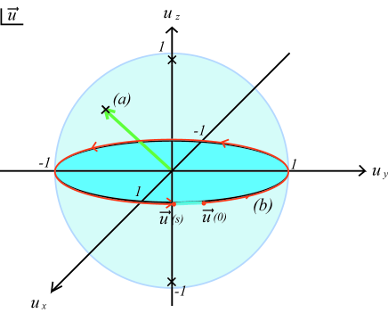
Figure 1: Classical solutions of eq.(29): (a) constant $\vec{u}$, (b) a path along a great circle on $S^{2}$.

Proof)

The theory has $O(3)\supset SO(3)$ global symmetry. Accordingly, one can take any initial value of $\vec{u}(0)$ for a classical solution. In other words, one may set $\vec{u}(0)$ to be the north pole for the representatives of the classical solutions, using two degrees of freedom of $SO(3)$ rotations. In addition, by $SO(2)$ local rotation symmetry or by one residual degree of freedom of $SO(3)$, we can freely set the orientation of $\partial\vec{u}(0)$. For example, $\left(\dot{\theta_{u}}(0),\dot{\varphi_{u}}(0)\right)=(0,a)$ or $(a,0)$. So, one may set the initial values as

$$\vec{u}(0) = (\theta_{u}(0),\varphi_{u}(0))=\left(\frac{\pi}{2},0\right),$$

$$\partial\vec{u}(0) = \left(\dot{\theta_{u}}(0),\dot{\varphi_{u}}(0)\right)=(0,a),$$ (31)

with a condition $a\geq 0$. The non-negative real constant $a$ turns out to be the only degree of freedom that represents all the classical solutions.

Substituting these initial values to the equations of motion (29), we obtain at $s=0$

$$\partial^{2}\theta_{u} = 0,\quad\partial^{2}\varphi_{u}=0.$$ (32)

So, an infinitesimal change $\epsilon$ of the variable $s$ yields

$$(\theta_{u}(\epsilon),\varphi_{u}(\epsilon))=\left(\frac{\pi}{2},\epsilon a\right),\quad\!\!\left(\dot{\theta_{u}}(\epsilon),\dot{\varphi_{u}}(\epsilon)\right)=(0,a).$$ (33)

As one can see in the equations of motion and in the above, so long as $\theta_{u}(s)=\frac{\pi}{2}$, eq.(32) holds at any $s$. Hence, the initial conditions leads to the pair of conditions, $\partial\theta_{u}(s)=0$ and $\theta_{u}(0)=\frac{\pi}{2}$. In other words, the pair of the conditions exhaust the representatives of the classical solutions. Thus, found solutions may well be regarded as the general solutions. $(Q.E.D.)$

Note that the solutions (30) can be regarded as ‘topological’ solutions in a sense that they are solitonic solutions.

IV.2 Non-local attractive interactions as a topological term

Now we consider the attractive interaction term (4). It is difficult to interpret it in the context of quantum theory due to its non-local nature along the polymer chain. However, we can solve them with our classical solutions (30). Let us rewrite eq.(4) with

$$\vec{r}(s)-\vec{r}(s^{\prime})=\int_{0}^{s}dt\,\vec{u}(t)-\int_{0}^{s^{\prime}}dt\,\vec{u}(t)=\int_{s^{\prime}}^{s}dt\,\vec{u}(t),$$

that is,

$$V_{AT}(s)=-W\int_{0}^{s}ds^{\prime}\;\delta\left(\int_{s^{\prime}}^{s}dt\,\vec{u}(t)\right).$$ (35)

Hence the problem is now reduced to the one in the $\vec{u}$ space: finding non-zero values of $\delta\left(\int_{s^{\prime}}^{s}dt\,\vec{u}(t)\right)$ with the classical solutions (30). That is to find $\vec{u}(s^{\prime})$ for a given $s$, which satisfies $\left|\int_{s^{\prime}}^{s}dt\,\vec{u}\right|=0$. Note that, exactly speaking, the integration over $s^{\prime}$ is from $0$ to $s-\epsilon$ with an infinitesimal positive constant $\epsilon$ (see Appendix A). Thus, we exclude the $s^{\prime}=s$ case in the following.

In the polar coordinates (20), this is expressed by

$$\int_{s^{\prime}}^{s}dt\,\sin\theta_{u}\cos\varphi_{u} = 0,$$

$$\int_{s^{\prime}}^{s}dt\,\sin\theta_{u}\sin\varphi_{u} = 0,$$

$$\int_{s^{\prime}}^{s}dt\,\cos\theta_{u} = 0.$$ (36)

The first classical solution ($\vec{u}=const.$) does not satisfy these equations and thus derives no attractive interactions. If we substitute the second classical solution of eq.(30) into eqs.(36), we have $\cos\theta_{u}(s)=0$,

$$\int_{s^{\prime}}^{s}\!\!\!dt\,\cos(at\!+\!b)\!\!\! = \!\!\!\frac{1}{a}\left(\sin(as\!+\!b)\!-\!\sin(as^{\prime}\!\!+\!b)\right)\!=\!0,$$

$$\int_{s^{\prime}}^{s}\!\!\!dt\,\sin(at\!+\!b)\!\!\! = \!\!\!\frac{1}{a}\left(\cos(as^{\prime}\!\!+\!b)\!-\!\cos(as\!+\!b)\right)\!=\!0.$$ (37)

Hence we have solutions: $s-s^{\prime}=2n\pi/a>0$, $n\in\mathbf{Z}$. Without any loss of generality, we assume $a>0$ and $n\in\mathbf{Z}_{+}$. Introducing $N(s)\equiv[as/2\pi]$ by Gauss’ symbol , we obtain

$$\int_{s-2\pi/a}^{s}dt\,\vec{u}(t)=\int_{s-4\pi/a}^{s}dt\,\vec{u}(t)$$

$$=\cdots=\int_{s-2\pi N(s)/a}^{s}dt\,\vec{u}(t)=0.$$ (38)

Therefore, the attractive potential is given by

$$V_{AT}(s)=-W\cdot N(s).$$ (39)

Note that $N(L)$ represents the winding number of the classical solution (30) along a great circle of $S^{2}$ (see Fig.1). Finally, an integration over $s$ yields the dimensionless Hamiltonian with our classical solutions:

$${\cal H} [\vec{u},W]=\int_{0}^{L}ds\,H(s)+\int_{0}^{L}ds\,V_{AT}(s)$$ (40)

$$= \frac{Ll}{2}a^{2}-W\left[\frac{2\pi}{a}\sum_{k=1}^{N(L)-1}k+\frac{2\pi}{a}\left(\frac{aL}{2\pi}-N(L)\right)N(L)\right]$$

$$= \frac{Ll}{2}a^{2}-WL\cdot N(L)\left\{1-\frac{\pi}{aL}\left(N(L)+1\right)\right\}.$$

The first term denotes the bending energy, and the second and the third terms are thought of as ‘topological’ terms from the winding number. When the chain of contour length $L$ winds $N(L)$ times we have the $N(L)$ circles of each length $\frac{2\pi}{a}$ and the rest $\left(L-\frac{2\pi}{a}N(L)\right)$. The second and third terms in the second line of eq.(40) result from the former and the latter respectively.

IV.3 The toroid and whip states

The non-zero winding number of the classical solution in the $\vec{u}$ space means that the polymer chain winds in the $\vec{r}$ space as well. That is, when $a>\frac{2\pi}{L}$, configurations around the second classical solution (30) start forming a toroidal shape since

$$\vec{r}(s)=\left(\begin{array}[]{c}\frac{1}{a}\left\{\sin(as+b)-\sin(b)\right\}\\ -\frac{1}{a}\left\{\cos(as+b)-\cos(b)\right\}\\ const.\end{array}\right),$$ (44)

and stabilise itself by attracting neighbouring segments. We call such classical solutions the “toroid states.” Whenever $a$ increases and passes through the point $\frac{2\pi n}{L}$ for $n\in\mathbf{Z}_{+}$, another toroid state appears with the increased winding number $n$. Note that the radius of the toroid state is given by $\frac{1}{a}$ (see Fig. 2).

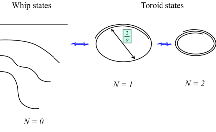
Figure 2: The whip ($N=0$) and toroid states ($N\geq 1$). The value of $b$ is given by the initial value of the bond vector $\vec{u}_{i}$.

When $0<a\leq\frac{2\pi}{L}$, the chain cannot wind like the toroid states. Both ends of the chain are not connected to each other, thus can move freely as well as any other parts of the chain fluctuate. As long as the total energy of the chain does not exceed the bending energy of $\frac{2\pi^{2}l}{L}$ at $a=\frac{2\pi}{L}$, they can whip with zero winding number.

We call such low-energy extended coil states the “whip states.” Although the definition includes fluctuations around the classical solutions, unless otherwise stated, we primarily refer to the classical solutions of such states, which are rather bowstrings than whips.

In the next subsection we explore the exact energy levels of the whip and toroid states, and discuss the phase transitions between these states.

IV.4 Favoured vacuum and toroid-whip transition

The dimensionless Hamiltonian of the second classical solution (30) is a function of $l,L,W$ and $a$:

$${\cal H}_{cl}(\!a,\!l,\!L,\!W\!)\!\equiv\!\frac{Ll}{2}a^{2}\!+\!\frac{\pi W}{a}N\!(\!L\!)\!\left(N\!(\!L\!)\!+\!1\right)\!-\!WL\!\cdot\!N\!(\!L\!).$$ (45)

This matches with the first classical solution when $\frac{N(L)}{a}=0$ for $a=0$ is defined. Accordingly, the above expression is valid for all classical solutions. Note that, since previous works assume a priori toroidal shape, no one clearly derived the precise microscopic Hamiltonian. Thus, we are now in a position to investigate exact energy levels of the whip and toroid states.

Consider first a case with $L$, $W$, and $l$ fixed. By definition, ${\cal H}(a)\equiv{\cal H}_{cl}(a,l,L,W)$ is continuous in the entire region of $a\geq 0$ and is a smooth function in each segment:

$$a\in\left[\frac{2\pi N}{L},\frac{2\pi(N+1)}{L}\right]\quad{\rm for~{}}N\in\mathbf{Z}_{\geq 0}.$$ (46)

However, it is not smooth at each joint of the segments: $\frac{aL}{2\pi}\in\mathbf{Z}_{+}$. Introducing a new parameter $c\equiv\left(\frac{L}{2\pi}\right)^{\!2}\!\frac{W}{2l}$ out of three existing degrees of freedom, we plot in Fig.3 the energy levels as a function of $a$ for different values of $c$, showing qualitative agreement with Conwell et al. for the condensation of $3$kb DNA in various salt solutions Conwell et al. (2003). Note that, in what follows, we call the segment (46) the “N-th segment” counting from $0$-th, and we also call $c$ the “conformation parameter” because the parameter $c$ solely determines the shape of this curve.

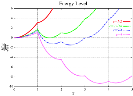
Figure 3: The dependence of the energy ${\cal H}(a)$ on $x=aL/2\pi$ and $c$. ${\cal H}(a)$ is scaled by the factor of $\sqrt{Wl}$ for convenience.

Suppose $N(L)=N$ is fixed, the Hamiltonian (45) takes a minimum at $a=a_{c}(N)\equiv\left(\frac{\pi W}{Ll}N(N+1)\right)^{1/3}$. Accordingly, each segment falls into one of the following three cases:

• When $a_{c}(N)\leq\frac{2\pi N}{L}$, ${\cal H}(a)$ is a monotonic function in the segment and takes its minimum at $a=\frac{2\pi N}{L}$.

• When $\frac{2\pi N}{L}<a_{c}(N)<\frac{2\pi(N+1)}{L}$, ${\cal H}(a)$ behaves quadratic in $a$ and takes its minimum at $a=a_{c}(N)$.

• When $\frac{2\pi(N+1)}{L}<a_{c}(N)$, ${\cal H}(a)$ is monotonic in the segment and takes its minimum at $a=\frac{2\pi(N+1)}{L}$.

The first and third cases are physically less relevant since they mean no (meta-)stable point in the segment. So, we focus on the second case.

The condition on $N$ for the second case turns out to be (see Fig. 4)

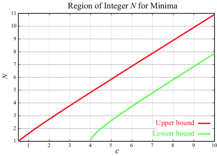
Figure 4: The solid line is the upper bound and the dashed line is the lower bound of $N$ for the minima, i.e., $N_{U,L}(c)$ (and $c_{U,L}^{(N)}$). The asymptotic values of $N_{U,L}(c)$ are both $N_{U,L}(c)\sim c$ ($c_{U,L}^{(N)}\sim N$).

$$N_{L}(c)< N <N_{U}(c)\quad{\rm for~{}}c\geq 4,$$

$$1\leq N <N_{U}(c)\quad{\rm for~{}}0\leq c<4,$$ (47)

where

$$N_{L}(c) \equiv \frac{c}{2}\left(1-\frac{2}{c}+\sqrt{1-\frac{4}{c}}\right),$$

$$N_{U}(c) \equiv \frac{c}{2}\left(1+\sqrt{1+\frac{4}{c}}\right).$$ (48)

Note that, by replacing $N$ with $N(L)=[aL/2\pi]$, one can read the condition on $a$ as well.

As one can see in Figs. 3, 4 , there are apparently more than one (meta-)stable toroid states at most values of $c$. This is because the first term of bending in eq.(45) is monotonically increasing, while the other two terms in eq.(45) are decreasing but not smoothly. This non-smoothness and the balance between two factors lead to multiple local minima and potential barriers between them. The number of minima is roughly given by the width of the region for $N$, i.e., $N_{U}(c)-N_{L}(c)$. For example, when $c\geq 4$,

$$N_{U}(c)-N_{L}(c) = 1+\frac{c}{2}\left(\sqrt{1+\frac{4}{c}}-\sqrt{1-\frac{4}{c}}\right)$$ (49)

$$= 1+\frac{c}{2}\left(\sum_{k=0}^{\infty}\frac{(-1)^{k}\left(-\frac{1}{2}\right)_{k}}{k!}\left(\frac{4}{c}\right)^{k}\right.$$

$$\,\,\,\,\,\,\,\,\,\,\,\,\,\,\,\left.-\sum_{k=0}^{\infty}\frac{\left(-\frac{1}{2}\right)_{k}}{k!}\left(\frac{4}{c}\right)^{k}\right)$$

$$= 3+2\left(\sum_{k=1}^{\infty}\frac{\left(\frac{1}{2}\right)_{2k}}{(2)_{2k}}\left(\frac{4}{c}\right)^{2k}\right)$$

$$> 3,$$

where $(a)_{k}=a(a+1){\cdots}(a+k-1)$ is the Pochhammer symbol. Therefore, there are at least three minima with positive winding numbers greater than 1. When $0<c<4$, the condition of having more than three minima is $c>\frac{9}{4}$. To summarise, when $c>\frac{9}{4}$ there exist at least three minima with positive winding numbers. It might be helpful to mention that, if we introduce the finite size effect in section VI, the number of minima could be reduced in some cases.

One can plot the critical value of $c$ where the minimum of the $N$-th segment emerges and vanishes. The lower bound of the $N$-th segment is

$$c_{L}^{(N)}=\frac{N^{2}}{N+1}<N,$$ (50)

while the upper bound is

$$c_{U}^{(N)}=\frac{(N+1)^{2}}{N}>N+1.$$ (51)

So, when $c$ satisfies the following inequality relation:

$$c_{L}^{(N)}\!\!<c<c_{U}^{(N)},$$ (52)

the $N$-th segment has a minimal and (meta-)stable point. For example, when $\frac{1}{2}<c<4$, the first segment $a\in[\frac{2\pi}{L},\frac{4\pi}{L}]$ (i.e. $N=1$) has a minimal point at $a=a_{c}(1)$.

Now we discuss the critical points of the conformation parameter $c$ at which the conformational transitions between states may occur. When $N_{U}(c)\leq 1$ (i.e. $c\leq\frac{1}{2}$), the second condition in eq.(47) vanishes and thus the whip states only survive at low energy. In this parameter region, the $a=0$ rod state will be favoured as the ground state with vanishing energy. Including ‘quantum’ fluctuations around $a=0$, we call this phase the whip phase. Successively, at the critical value of $c=\frac{1}{2}$, the whip phase to whip-toroid co-existence phase transition would occur. On the other hand, when $c>\frac{1}{2}$, there always exists at least one (meta-) stable toroid state with positive winding number $N(L)$. As $c$ grows over $\frac{1}{2}$, the local minimum in the first segment decreases from some positive value. Finally, when the energy of the $N=1$ stable toroid state balances with the ground state of the whip state (i.e. ${\cal H}_{cl}=0$), the whip-dominant to toroid-dominant phase transition may occur. Such a value of $c$ is $27/16$. Since there is a potential barrier between the $a=0$ rod and the $N=1$ stable toroid states, the transition is first order. When $c>27/16$, the toroid states will dominate the action. The energy plot (Fig. 3) clearly shows that the transitions between the toroid states are also first order, if any, as there exist potential barriers between two successive minima. Further discussions on the phase transitions will be given in the final section.

For later convenience, we rewrite the Hamiltonian (45) and $a_{c}(N)$ in terms of $c$ and the new variable $x\equiv\frac{aL}{2\pi}$

$${\cal H}_{cl}(a,l,L,W)=\frac{WL}{2}{\cal H}(c,x)$$

$$=\sqrt{2\pi^{2}Wl}\left\{\sqrt{c}\;{\cal H}(c,x)\right\}=\frac{4\pi^{2}l}{L}c\;{\cal H}(c,x),$$ (53)

where

$${\cal H}(c,x) = \frac{x^{2}}{2c}+\frac{1}{x}[x]([x]+1)-2[x].$$ (54)

Therefore, $[x]=N(L)$ and $x_{c}([x])=\frac{a_{c}(N)L}{2\pi}=\left\{c\cdot[x]([x]+1)\right\}^{1/3}$.

V Stability, quantum fluctuations, and perturbations

So far we have dealt with the classical solutions, which are derived from the first derivative of the action. Thus, they may correspond to the global/local minima of the action in the configuration space. However, the solutions are not necessarily stable unless we take into account the attraction, since the second derivative test of the action with $W=0$ gives the non-positive Hessian. That is to say, they seem to be saddle points.

$$\left.\frac{\delta^{2}S[\theta_{u},\varphi_{u}]}{\delta\varphi_{u}^{2}}\right|_{W=0} = 0,$$

$$\left.\frac{\delta^{2}S[\theta_{u},\varphi_{u}]}{\delta\theta_{u}^{2}}\right|_{W=0} = \left(l\dot{\varphi}_{u}^{2}\right)\cos 2\theta_{u},$$

$$\left.\frac{\delta^{2}S[\theta_{u},\varphi_{u}]}{\delta\theta_{u}\delta\varphi_{u}}\right|_{W=0} = -l\left(2\dot{\theta}_{u}\dot{\varphi}_{u}\cos(2\theta_{u})+\ddot{\varphi}_{u}\sin(2\theta_{u})\right),$$

$$\det H|_{W=0} = \left|\begin{array}[]{cc}\partial_{\varphi}^{2}S&\partial_{\varphi}\partial_{\theta}S\\ \partial_{\theta}\partial_{\varphi}S&\partial_{\theta}^{2}S\end{array}\right|_{W=0}\leq 0$$ (57)

In fact, the general whip states do not need to live in a flat plane in $\mathbf{R}^{3}$ whereas the classical whip state does. So, the transitions between the classical and the non-classical whip states have the flat directions, i.e., they can be seamless without any change of energy. Therefore, the stability problem is to be treated carefully with and without attraction.

V.1 Stability and quantum fluctuations with attraction

When the attraction is turned on, the toroid states with the winding number of more than two may become extremely (meta-)stable under the quantum fluctuations away from the classical solutions. It is not easy to show that all such second derivatives of the action give positive values and therefore stabilise the states, since the interaction term contains a special function of the quantum variable $\vec{u}$. However, there is a much easier way to see the stability.

Consider any small fluctuation of a segment $\delta l_{s}$ from such a state. It gives rise to an increase of the energy:

$$\delta{\cal H}(a)\geq W\cdot\delta l_{s}.$$ (58)

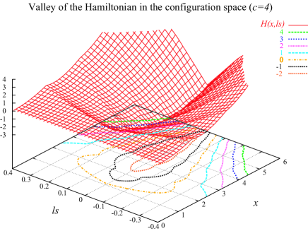
Figure 5: A sketch of the energy level ${\widetilde{\cal H}}(x,l_{s})$ with the attraction. For ease of use, the maximum value is suppressed at $4$ and $l_{s}$ is normalised by $L$. The direction along the valley is parameterised by $a$ variable of the classical solution. Its perpendicular direction is the quantum fluctuation $l_{s}$ by $SO(2)$ away from the classical solutions. As one can see, $l_{s}$ is a flat direction for the whip states $(x<1)$.

More generally, we can write down the dimensionless Hamiltonian as a function of $a$, or $x$, and $l_{s}$, that is, the energy levels away from the toroid states. $l_{s}$ is now defined as the length $l_{s}$ of the polymer segment shifted from an end of the toroid. The shifted polymer segment is locally rotated by $SO(2)$ transformation, for example, by $90$ degrees at each node, keeping the local bending energy unchanged.

$${\cal H}(a,l_{s}) = {\widetilde{\cal H}}(x,l_{s})$$ (59)

$$= \frac{WL}{4c}x^{2}+\frac{WL}{2x}[x(1-\frac{l_{s}}{L})]\left([x(1-\frac{l_{s}}{L})]+1\right)$$

$$-WL[x(1-\frac{l_{s}}{L})]+Wl_{s}[x(1-\frac{l_{s}}{L})],$$

where $x=\frac{aL}{2\pi}$ (Fig.5). The energy loss for the infinitesimal segment $\delta l_{s}$ is found to be

$$\delta E=WN\delta l_{s},$$ (60)

where $N$ is the local number of the overlapped segments $N=[\frac{a(L-l_{s})}{2\pi}]$. When $l_{s}=L$, the energy becomes $E=\frac{Ll}{2}a^{2}$ of the bending energy.

Therefore, under perpendicular ‘quantum’ fluctuations away from the classical solutions, the toroid states which look stable in ${\cal H}_{cl}$ are also generally (meta-)stable. It should be noted here that the fluctuation along the classical solutions may still be flat so that the transitions from one toroid state to another is possible. These facts justify our claims on the phase transitions between toroid states and their existence.

As for the toroid state with the winding number one, its stability depends on the value of $c$. The transition along the classical solutions is almost flat so that when $c\leq\frac{1}{2}$ it naturally goes down to a whip state (Fig.5). Therefore, it is absolutely unstable. When $c>\frac{1}{2}$, one may state that it is meta-stable since attracted parts locally stabilise the state. However, the non-attracted parts are still free to move unless it gives an increase of the total energy. So, the toroid state with $N=1$ is partially stable or metastable. Its probability is given by summing over such quantum fluctuations of non-attracted parts that give the energy similar to that of the classical solution.

On the other hand, even with the attraction, the whip state is unstable since it is not affected by the presence of the attraction. Therefore, it would be meaningless to pick up any particular shape of the whips and estimate its probability. Instead, one should only estimate the probability of all the whip states that have the similar energy ${\cal H}(a<2\pi/L)$, by carefully counting the number of such states, or equivalently by estimating entropy. Note that, roughly speaking, the whip state is more probable than a single rod state with $a=0$.

With the above reasons, it would be more appropriate to state that one of the toroid states of $N=[x]\geq 2$ is the ground state when $l$ is much larger than the bond length $l_{b}$ and $c\geq 4$ where the whip states become negligible. Although we listed the above reasons, we remind that there is a first order transition between the rod ($a=0$) and the toroid state ($N=1$). The potential barrier between them is given by $\frac{2\pi^{2}l}{L}$, thus the transition will be suppressed by the factor of $e^{-1}$ or smaller when $L<2\pi^{2}l\sim 1\mu m$ in the case of DNA with $l\sim 50nm$.

V.2 Perturbation by the classical solutions

In order to complete the theory at low energy, we construct the low-energy effective Green function $G_{eff}$ from those of the toroid and the whip states, in perturbation theory. To make the function more accessible, we fix the persistence length $l$ in what follows. Accordingly, $G_{eff}$ becomes a function of $L$ and $W$, or equivalently, of $c$ and $L$. In addition, $c=\frac{W}{2l}\left(\frac{L}{2\pi}\right)^{2}\geq 4$ is assumed to ensure the existence of the stable toroid states at the beginning.

Let us denote the Green function of the toroid states by $G_{T}$, and that of the whip states by $G_{w}$. As we would like to sum over all toroid contributions to $G_{T}$, the end-to-end vector $\vec{R}$ and the initial and final bond vectors $(\vec{u}_{i},\vec{u}_{f})$ will be omitted in $G_{T}$ as well as in $G_{w}$. Therefore, $G_{T}$ is a function only of $c=c(\tau)$ where $c(\tau)$ is a function of the chain length $\tau$ of the toroidal segment. $G_{w}$ is also a function of $\tau$: the length of the non-attracted whipping segment in this case. Note that, however, $G_{w}(\tau)$ does not depend on $W$ since the chain segment is free by definition.

With these specifications, the effective Green function can be constructed by the following perturbations:

$$G_{eff}(c,L)=G_{w}(L)$$

$$+\Biggl{[}G_{T}(c(L))+2\int_{0}^{L-L_{min}}d\tau\;\;G_{T}(c(L-\tau))\,G_{w}(\tau)$$

$$\qquad+\int_{\tau_{1}>0,\tau_{2}>0,\atop\tau_{1}+\tau_{2}<L-L_{min}}d\tau_{1}d\tau_{2}\;\;G_{w}(\tau_{1})\,G_{T}(c(L-\tau_{1}-\tau_{2}))\,G_{w}(\tau_{2})\Biggr{]}$$

$$+\Biggl{[}\int_{L_{min}}^{L-L_{min}}d\tau\;\;G_{T}(c(L-\tau))\,G_{T}(\tau)$$

$$\qquad+2\int_{\tau_{1}>L_{min},\tau_{2}>0,\atop\tau_{1}+\tau_{2}<L-L_{min}}d\tau_{1}d\tau_{2}\;\;G_{T}(c(L-\tau_{1}-\tau_{2}))\,G_{T}(\tau_{1})\,G_{w}(\tau_{2})$$

$$\qquad+\int_{\tau_{1}>0,\tau_{2}>L_{min},\atop\tau_{1}+\tau_{2}<L-L_{min}}d\tau_{1}d\tau_{2}\;\;G_{T}(c(L-\tau_{1}-\tau_{2}))\,G_{w}(\tau_{1})\,G_{T}(\tau_{2})$$

$$\qquad+\int_{\tau_{1,3}>0,\tau_{2}>L_{min},\atop\sum_{i=1}^{3}\tau_{i}<L-L_{min}}\left[\prod_{i=1}^{3}d\tau_{i}\right]\;G_{w}(\tau_{1})\times$$

$$\,\,\,\,\,\,\,\,\,\,\,\,\,\,\,\,\,\,\,G_{T}\left(c\left(L-\sum_{i=1}^{3}\tau_{i}\right)\right)\,G_{T}(\tau_{2})\,G_{w}(\tau_{3})$$

$$\qquad+2\int_{\tau_{1,3}>0,\tau_{2}>L_{min},\atop\sum_{i=1}^{3}\tau_{i}<L-L_{min}}\left[\prod_{i=1}^{3}d\tau_{i}\right]G_{T}\!\left(\!c\!\left(\!L\!-\!{\textstyle\sum_{i=1}^{3}\!\tau_{i}}\!\right)\right)\!\times\!$$

$$\,\,\,\,\,\,\,\,\,\,\,\,\,\,\,\,\,\,\,G_{w}(\tau_{1})\,G_{T}(\tau_{2})\,G_{w}(\tau_{3})$$

$$\qquad+\int_{\tau_{1,2,4}>0,\tau_{3}>L_{min},\atop\sum_{i=1}^{4}\tau_{i}<L-L_{min}}\left[\prod_{i=1}^{4}d\tau_{i}\right]\;G_{w}(\tau_{1})\times\,$$

$$\,\,\,\,\,\,\,\,\,\,\,\,\,\,\,\,\,\,\,G_{T}\left(c\left(L-\sum_{i=1}^{3}\tau_{i}\right)\right)\,G_{w}(\tau_{2})\,G_{T}(\tau_{3})\,G_{w}(\tau_{4})\Biggr{]}$$

$$+\cdots,$$ (61)

where $L_{min}$ is given by the lower bound of the conformation parameter $c$: $c(L_{min})=1/2$, for the existence of a (meta-)stable toroid state. It reads

$$L_{min}=\frac{L}{\sqrt{2c(L)}}=2\pi\sqrt{\frac{l}{W}}.$$ (62)

The first bracket in eq.(61) gives the contributions from the conformations which contain only one toroid, the second bracket gives the ones with two toroids, and so on. It should be noted that so-called ‘tadpole’ conformation appears in this low energy perturbation as the third term in eq.(61) with one toroid and one whip. Schematically, eq.(61) can be depicted in Fig.6.

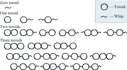
Figure 6: Each term in eq.(61) is expressed by a product of the toroids (circles) and the whips (waves). The third term is so called the ‘tadpole’ conformation. Below the forth term, all contributions are of multi-tori.

Roughly speaking, in our ideal toroid with zero thickness, the winding number $N_{c}$ of the dominant toroid state is proportional to $c(\tau)$ which is a quadratic function in $\tau$. Besides, the minimum of the Hamiltonian is given at $a_{c}(N_{c})$: ${\rm Min}({\cal H}(a))\sim-\frac{WLN_{c}}{4}\sim-\frac{\pi{W^{2}}}{4l}\!{\left(\frac{L}{2\pi}\right)}^{\!3}$. Therefore, the ratio of the probabilities of the toroids with different lengths $\tau$ and $L$ can be estimated by

$$\frac{G_{T}(c(\tau))}{G_{T}(c(L))}\sim\frac{e^{\frac{\pi W^{2}}{4l}\left(\frac{\tau}{2\pi}\right)^{3}}}{e^{\frac{\pi W^{2}}{4l}\left(\frac{L}{2\pi}\right)^{3}}}=e^{-\frac{W^{2}}{2^{5}\pi^{2}l}\left(L^{3}-\tau^{3}\right)}.$$ (63)

Since we assume that $L$ is large enough as $L^{3}\gg\frac{2^{5}\pi^{2}l}{W^{2}}$, the toroid states with smaller contour length are highly suppressed by the above factor (From $c{\geq}4$, we have $L^{3}\geq{\left(2^{5}{\pi}^{2}lW\right)}^{\frac{1}{2}}\left(\frac{2^{5}\pi^{2}l}{W^{2}}\right)$. If $W{\sim}O(1)$ and $l{\gg}1$, we obtain $L^{3}\gg\frac{2^{5}\pi^{2}l}{W^{2}}$).

For example, this condition holds for the cases of DNA considered in the next section. Hence, the above perturbation can be justified for a large value of $c(L)$. Note, however, that the statistical weight for each path, or each conformation, is not specified here, nor for the whip state and the normalisation factor. Moreover, we have not counted other conformations such as conventional ‘tadpoles’ with overlaying whips. Therefore, and unfortunately, we do not go into the precise comparison of the above terms. Instead, we will make some remarks on these issues in the final section.

VI Comparison with experiments

In previous sections, we have found the toroid states as the classical solutions and found that some of them are (meta-)stable, one of which becomes the ground state at large $c$. As mentioned, it is pointless to ask $\vec{u}_{i},\vec{u}_{f}$, and $\vec{R}(L)$. One of the most physically meaningful observable is the radius of the toroid.

For large $c$, the ground state — the dominant toroid state of the winding number $N_{c}$ can be estimated by the inequality relation (52) of $c$:

$$c_{L}^{(N_{c})}<c<c_{U}^{(N_{c})}.$$

By its inverse relation, it reads $N_{c}\simeq c$, since $c_{L}^{(N_{c})}\simeq N_{c}$ and $c_{U}^{(N_{c})}\simeq N_{c}$. Using this, we can estimate that the radius of our dominant ideal toroid behaves

$$r_{c}=\frac{L}{2\pi N_{c}}=\frac{4\pi l}{WL}.$$ (64)

This result is, however, not directly applicable to the physical systems, because our model has the zero thickness of the chain. That is, every chain segment interacts equally with all the other segments accumulated on the same arc of the toroid.

Therefore in this section, we first introduce a finite size effect into our Hamiltonian. We then estimate the mean radius of toroid and compare resulting analytical expression with the experiments of DNA condensation Yoshikawa et al. (1999); Bloomfield (1996). Also, the mean radius of the toroid cross section is calculated in the end.

VI.1 Finite size effect

The finite size effect of the toroid cross section can be approximated by the hexagonally arranged DNA chains with van der Waals type interactions, i.e., with the effective nearest neighbour interactions. Namely, if the chains are packed in a complete hexagonal cross section, the winding numbers are $N=7,19,37$, and so on. In such cases, the number of van der Waals interactions between segments can be counted by the links between neighbouring pairs in the hexagonal cross section. We then obtain the number as a discrete function ${\cal V}_{discrete}(N)$. We can approximate it or analytically continue to the following analytic function ${\cal V}(N)$:

$${\cal V}(N)=3N-2\sqrt{3}\sqrt{N-\frac{1}{4}}.$$ (65)

Thereupon, the attractive energy can be expressed by those of $N$ loops and the rest of the chain:

$$\int_{0}^{L}\!\!\!\!ds\;V_{AT}(s)\!=\!-\frac{2\pi{W}}{a}{\cal V}(N)\!-\!W\!\!\left(\!\!L\!-\!\frac{2\pi N}{a}\!\right)\!Gap(N),$$ (66)

where $Gap(N)\equiv{\cal V}(N+1)-{\cal V}(N)$ is additionally introduced in order to compensate the continuity of the potential as a function of $a$. Note that, up to $N=3$, we need not to introduce this finite size effect, since there is no difference between the ideal toroid and the hexagonally arranged case: the number of links are the same in both cases. Therefore, we assume $N(L)\geq 4$ for this effect. Note also that the entanglement (knotting) effect of the chain arrangement is neglected.

Finally, substituting eq.(66) into ${\cal H}[\vec{u},W]$, the finite size effect leads to the modified Hamiltonian:

$${\cal H}(a) = \frac{Ll}{2}a^{2}-\frac{2\pi W}{a}{\cal V}(N(L))$$ (67)

$$-\frac{2\pi W}{a}\!\left(\frac{aL}{2\pi}-N(L)\right)Gap(N(L)).$$

Most physical observables for tightly packed toroids can be quite accurately estimated using this Hamiltonian. For example, in principle, we can derive the exact value of the radius of the stable toroid. In fact, by the same analysis presented in the previous section, we obtain the following “asymptotic” relation of $N_{c}$ of the dominant toroid for large $c$:

$$N_{c}\simeq\left(2\sqrt{3}\,c\right)^{\frac{2}{5}}.$$ (68)

VI.2 Mapping onto experimental data

By $r_{c}\equiv\frac{L}{2\pi N_{c}}$, we now estimate the mean radius of the toroid (i.e. the average of inner and outer radii) in a physical system. A coupling constant of (4) can be given by $W\!=\!\frac{1}{l_{m}}\!\!\left(\frac{k\epsilon}{k_{B}T}\right)$ where $k$ is the number of the electric dipoles in a monomer segment, each of which creates van der Waals interaction of the magnitude $\epsilon$. $l_{m}$ denotes the length of the monomer along the chain contour, taken to be a half of pitch per turn (of helix) $l_{m}\simeq 5\,bp=1.66\,nm$ in the end. Note we assume $l_{m}\sim l_{b}$. Substituting $N_{c}$ of the dominant toroid state (68) and the above, we obtain

$$r_{c}\simeq{\left(6\pi\right)}^{-\frac{1}{5}}L^{\frac{1}{5}}{\left(\frac{l}{W}\right)}^{\!\!\frac{2}{5}}\!\!=\!{\left(6\pi\right)}^{-\frac{1}{5}}L^{\frac{1}{5}}{\left(l_{m}l\right)}^{\frac{2}{5}}{\left(\frac{k\epsilon}{k_{B}T}\right)}^{\!\!-\frac{2}{5}}\!\!\!\!\!\!\!.$$ (69)

The scaling property of the first equality matches with the one in Stukan et al. (2003). Note that a coupling constant of second nearest neighbour is vanishingly small $W_{2}\,{\simeq}\,2^{-6}W=\frac{1}{64}W$, so that one may neglect it in this van der Waals regime.

We estimate the mean toroidal radius of T$4$ DNA in low ionic conditions reported in Yoshikawa et al. (1999). Using $L=57{\mu}m$, $l\,{\simeq}\,50\!\sim\!60\,nm$, and $l_{m}$, the mean radius of the toroid is

$$r_{c}=29.09B^{-\frac{2}{5}}\sim 31.29B^{-\frac{2}{5}}{~{}[nm]},$$ (70)

where $B\equiv\frac{k\epsilon}{k_{B}T}$. This is in good agreement with the experiment $r_{c}\simeq 28.5$ $nm$ for $B\,{\sim}\,1.15$.

The same argument for the toroid formed by Sperm DNA packaged by protamines Bloomfield (1996) ($L=20.4{\mu}m$), gives the analytic value

$$r_{c}=23.69B^{-\frac{2}{5}}\sim 25.48B^{-\frac{2}{5}}~{}[nm],$$ (71)

which also agrees with an experimental result $r_{c}{\simeq}26.25$ $nm$ for $B\,{\sim}\,0.85$. Note that the former toroid is densely packed Yoshikawa et al. (1999), hence hexagonal assumption could be a good approximation. It is therefore well expected to have the stronger attraction compared to thermal fluctuations, $B>1$. The latter has a larger diameter of the effective segment. Thus, it may well be expected to have the weaker but large enough interaction with smaller $B$ to maintain a toroidal conformation.

Similarly, the mean radius of the toroid cross section can be calculated for the complete hexagonal cross section with a side of $n$ monomers:

$$r_{cross}=\frac{2+\sqrt{3}}{4}\left(n-\frac{1}{2}\right)l_{d}$$ (72)

where $l_{d}$ is the diameter of the segment. Substituting our relation of $n$ with the winding number $N$: $n=\frac{1}{2}+\frac{1}{\sqrt{3}}\sqrt{N-\frac{1}{4}}$, eq.(72) can be rewritten as

$$r_{cross}=\frac{2\sqrt{3}+3}{12}N^{\frac{1}{2}}\left[1-\frac{1}{8N}+O\left(\frac{1}{N^{2}}\right)\right]l_{d}.$$ (73)

Using this general result, we now specify the type of interactions and derive the expression for the mean radius of the toroid cross section. In the case of van der Waals interactions, $N_{c}$ is given by eq.(68), and therefore we have

$$r_{cross} \simeq \frac{3\sqrt{3}+6}{12}{\left(6\pi\right)}^{\!-\frac{2}{5}}\!L^{\!\frac{2}{5}}\!{\left(\frac{W}{l}\right)}^{\!\!\frac{1}{5}}\!\!l_{d}$$ (74)

$$= \frac{3\sqrt{3}+6}{12}{\left(6\pi\right)}^{\!-\frac{2}{5}}\!L^{\frac{2}{5}}{\left(l_{m}l\right)}^{\!\!-\frac{1}{5}}\!{\left(\frac{k\epsilon}{k_{B}T}\right)}^{\!\!\frac{1}{5}}\!\!l_{d}.$$

Note that the scaling property $r_{cross}\sim L^{\frac{2}{5}}$ is in agreement with the one in Stukan et al. (2003) obtained in the asymptotic limit.

Similarly, we can formally consider the case of ideal toroid, although it has zero thickness. In this case with $N_{c}\simeq c$, we have

$$r_{cross} \simeq \frac{2\sqrt{3}+3}{24\pi}L{\left(\frac{W}{2\,l}\right)}^{\!\!\frac{1}{2}}\!l_{d}$$ (75)

$$= \frac{2\sqrt{3}+3}{24\pi}\,L\,{\left({2\,l_{m}l}\right)}^{\!-\!\frac{1}{2}}\!{\left(\frac{k\epsilon}{k_{B}T}\right)}^{\!\!\frac{1}{2}}\!l_{d}.$$

It should be noted that, with van der Waals interactions, the mean radius of the toroid scales as $L^{\frac{1}{5}}$ while that of the toroid cross section scales as $L^{\frac{2}{5}}$. In the case of ideal toroid, the mean radius of the toroid scales as $L^{-1}$ while that of the cross section scales as $L$.

VII Discussion and concluding remarks

We have shown that the (meta-)stable toroid states appear as the classical solutions of the low energy effective theory of a semiflexible homopolymer chain — the nonlinear sigma model on a line segment. We have shown in this paper the complete proof of the statement that our classical solutions represent the general solution. The novelty of the model comes from the fact that the difficulties of the local inextensibility constraint $|\vec{u}|^{2}=1$ and the delta-function potential are resolved explicitly with our solutions in the path integral formulation (hence our theory goes further beyond the Gaussian approximation). Together with our microscopic Hamiltonian, they lead us to the profound analytic curve of the energy levels (Fig.3). It is also of interests that the balance between the bending energy and the attractive potential creates multiple local minima at $a=a_{c}(N)$ for each $N$ satisfying eq.(47). One can read off from eq.(49) and Fig.4 that the number of local minima is basically three or four in the case of our ideal toroid. Another work on multiple local minima will be mentioned shortly. In search of the ground state, we found that the phase transitions occur at $c=\frac{1}{2}$ and at $c=\frac{27}{16}$, and discovered that such configurational transitions are governed by the conformation parameter $c=\frac{W}{2l}\left(\frac{L}{2\pi}\right)^{2}$. The critical point $c=\frac{27}{16}$ indicates the whip-toroid or whip-dominant to toroid-dominant transition of the first order.

In section V-A, we have shown the stability of the toroid states and the validity of such phase transitions. We also calculated the potential barrier of the whip-toroid transition (rod-toroid transition), and indicated that, for the chains of $L<1$ $\mu m$, the rod ($a=0$) to $N=1$ (meta-)stable toroid state transition is fairly unlikely. This would explain why it is difficult to observe short DNA toroids in experiments T05 (2005). In section V-B, we have constructed the effective Green function from those of the whip and toroid states using perturbation theory at low energy. It naturally contains multi-tori and ‘tadpole’ conformations.

We finally introduced the hexagonal approximation to count the finite size effect of the toroid cross section and established the mapping onto the experimental data of the DNA toroid radii. Our result is even quantitatively in good agreement with the experiments Yoshikawa et al. (1999); Bloomfield (1996). Hence, we conclude that our theory is certainly an analytic theory of DNA condensation and of toroidal condensation of many other semiflexible polymer chains with effective van der Waals attraction, or equivalently with effective short-range dominant attraction. Here, we presented only the comparisons with DNA condensations, but simply by varying the parameters $l,W,L$, and $l_{m}$, our theory and results should fit to the same problems in similar biochemical objects.

In analogy to the classical limit $\frac{1}{\hbar}\to\infty$ in quantum mechanics, it is assumed that the persistence length $l$ is large enough for our low energy theory to be valid. The local inextensibility constraint is originally given by some bond potential such as $\lambda(|\vec{u}|-1)^{2}$ with the spring constant $\lambda$. Note the low energy theory becomes invalid when the constraint does not hold in the Hamiltonian. That is, $l$ and $\lambda$ should be sufficiently larger than $O(1)$ so that our theory remains valid. On the other hand, as $l$ approaches $1$ or $0$, one may be able to see the transition from whip-toroid phase to coil-globule or coil-rod phase. This is beyond our scope in this paper, but the issue will be discussed at the end of this section.

Of particular interest on multiple local minima is the work by Kuznetsov and Timoshenko Kuznetsov and Timoshenko (1999). Using Gaussian variational method and off-lattice Monte Carlo simulation, they numerically calculated the phase diagram for a ring semiflexible chain in various solvent conditions. Note that their model Hamiltonian is the same as ours except for the harmonic spring term connecting adjacent beads. For a given stiffness, upon increasing the magnitude of two-body attraction, they found toroids with larger winding numbers become more stable. This is consistent with our findings as our conformational parameter $c$ is a function of the magnitude of the attraction $W$. They also found that several distinct toroid states (i.e. multiple minima) can exist, which are characterized by winding numbers and are separated by first order phase transition lines (see Fig.$4$ in Kuznetsov and Timoshenko (1999)). Although they considered a ring polymer, these facts are in good agreement with our analytic findings for an open semiflexible chain. It would be of great interest to numerically check the existence of multiple minima for an open semiflexible chain.

So far, we have only dealt with the whip and toroid conformations, but there are other configurations to be explored. Numerical simulations showed that a semiflexible chain takes toroid, collapsed rod or racquet conformations, depending on chain length, stiffness, magnitude of interactions, temperature, and other variables. Of particular interest is the works by Noguchi et al. Noguchi and Yoshikawa (1998); Noguchi et al. (1996) and Stukan et al. Stukan et al. (2003); Martemyanova et al. (2005) who studied the dependence of stiffness on conformational properties. They observed both toroid and collapsed rod states for some intermediate stiffness. Upon increasing stiffness they found toroid states are more probable.

Collapsed rods have not been present in our model. One of the reasons is they are not classical solutions, which can only survive and become the only candidates for the ground state at large $l$ or at small $T$. Another reason may be because the inextensibility constraint $|\vec{u}|^{2}=1$ is quite strong or because collapsed rods are energetically less favoured. That is, our model with the constraint is simply in the quite stiff regime where the collapsed rods are less likely. Moreover, discrete nature of the chain, which are present in most numerical models, might allow sudden hairpins although they are highly disfavoured in some continuum models. Indeed, when they increase stiffness, toroid states are more probable Noguchi and Yoshikawa (1998); Martemyanova et al. (2005). This competition in the intermediate stiffness remains an interesting open question.

In addition to toroids and collapsed rods, tadpole like conformations (i.e. a toroid head with long tail) have been observed in the experiment by Noguchi et. al. Noguchi and Yoshikawa (1998). They also performed the Monte Carlo simulations and found that this tadpole like structure was realised only twice in a hundred runs. We have also dealt with a ‘tadpole’ conformation in the effective Green function, but it only includes the simplest tadpole shape: a toroid with a single non-interacting whip. Therefore, we have not counted tadpoles such as a toroid with two whips attracting each other or a toroid with a collapsed rod or a toroid with two collapsed rods attracting each other. To compare them, one should first estimate the entropy of the whip and compare it to the toroids. Also, relative energy levels and statistical weights of these conformations (toroid, collapsed rod, tadpole) including reported racquet states of metastable intermediate Martemyanova et al. (2005); Schnurr et al. (2000, 2002) will be studied in the forthcoming work. Note that the whip is defined by the elongated state at low energy whose upper bound is given tentatively by $E<\frac{2\pi^{2}l}{L}$. Precisely speaking, it should be the lowest bound for a chain to form a loop, which is to be explored in detail as well as the above.

As for the scaling property $r_{c}\sim L^{\nu}$ of the toroid radius, the exponents $\nu$ predicted in the literature in the asymptotic limit are $\nu=\frac{1}{5}$ in most cases Stukan et al. (2003); Schnurr et al. (2002); Pereira and Williams (2000); Miller et al. (2005). This agrees with our precise asymptotic result (69) where both the parameter $c$ and the winding number $N_{c}$ of a dominant toroid are large enough. Note our model has robustness in that it can treat chains of any finite length: a real chain is a finite system.

However, the exponents are inconsistent with the experimentally well known observation that the radius is independent of the chain length Bloomfield (1991, 1996); Yoshikawa et al. (1999). This might suggest that the real interaction is not necessarily van der Waals like, or at least is not a single van der Waals type interaction. It should be noted here that combinations of our ideal toroid and its finite size effect can give a range of $\nu=-1\sim\frac{1}{5}$ in some region.

Another interesting remark is that when we apply Coulomb like interactions to our approximation, we observe the radius remains nearly constant as $L$ changes. This will be presented in the near future Ishimoto and Kikuchi (2006b).

Finally, we remark that our model can be regarded as the linear sigma model at low energy where it actually reduces to the nonlinear sigma model. The linear sigma model is one of the most suitable models to describe phase transitions in quantum field theory. Although we are not formulating quantum field theory, the model actually involves a phase transition from a constrained to non-constrained system, that is, from constant-length bonds to spring-like bonds (Gaussian flexible chain). This is an interesting model to be studied. Although we have listed some questions to solve, there are obviously a lot of problems to be investigated. Our theory could also be extended and applied to the challenging interdisciplinary problems such as protein folding.

Acknowledgments

We are grateful to K. Binder, V. A. Ivanov, W. Paul, and N. Uchida for their stimulating discussions. Y.I. is grateful to K. Nagayama for his discussions and encouragement, and to T. Araki for his comment. N.K. is grateful to H. Noguchi, A. Cavallo and T. Kawakatsu for stimulating discussions, and to T. A. Vilgis for his earlier discussions of the field theory of globule-toroid transition which led us to this direction. Y.I. acknowledges the Yukawa Institute for Theoretical Physics where this work is partially done during the YITP-W-05-04 Workshop “Soft Matter as Structured Materials”. N.K. acknowledges the Deutsche Forschungsgemeinschaft for financial support.

Appendix A The delta function potential

Our delta function potential expressed in the body is

$$V_{AT}(s)=-W\int_{0}^{s}ds^{\prime}\;\delta\left(\vec{r}(s)-\vec{r}(s^{\prime})\right).$$ (76)

This is, however, rather schematic. The precise definition will be given below, sorting out two ambiguities in eq.(76). One is the definition of the delta function and the other is its integration contour concerning the self-interaction contribution. The exact form of the function is given by renormalising the coupling constant, the measure, or the delta function itself appropriately, and by expecting some ultraviolet (short-range) cutoff $\epsilon>0$ in the integration contour:

$$V_{AT}(s)=-W\!\!\int_{0}^{s-\epsilon}\!\!\!\!\!\!\![ds^{\prime}]_{re}\;\delta\left(\left|\vec{r}(s)-\vec{r}(s^{\prime})\right|\right)\,\,\,{\rm for~{}}\epsilon\leq s,$$ (77)

otherwise it vanishes.

First, we should interpret that the delta function is not three-dimensional but one-dimensional, changing its argument from $\left(\vec{r}(s)-\vec{r}(s^{\prime})\right)$ to $\left|\vec{r}(s)-\vec{r}(s^{\prime})\right|$. When the argument of the delta function has some zeros, it has the following property. Say that the argument is given by a function $g(x)$ then

$$\delta\left(g(x)\right)=\sum_{x_{i}}\frac{\delta(x-x_{i})}{|g^{\prime}(x_{i})|}$$ (78)

where $\{x_{i}\}$ is the roots of $g(x)$. Accordingly, at around every zero, the integration over $x$ gives a $|g^{\prime}(x_{i})|^{-1}$ contribution. By definition, our potential should not have such a contribution, so that the amplitude must be normalised appropriately. For example, such a renormalisation of the measure can be achieved by

$$\int_{-\infty}^{\infty}[dx]_{re}\;\delta\left(g(x)\right) = \int_{-\infty}^{\infty}[dx]_{re}\;\sum_{x_{i}}\frac{\delta(x-x_{i})}{|g^{\prime}(x_{i})|}$$ (79)

$$= \sum_{x_{i}}\int_{x_{i}}dx|g^{\prime}(x_{i})|\;\frac{\delta(x-x_{i})}{|g^{\prime}(x_{i})|}$$

$$= \sum_{x_{i}}\int_{x_{i}}dx\;\delta(x-x_{i})$$

$$= {\rm Number~{}of~{}zeros}.$$

As given in the second line of the above expression, the measure is renormalised such that it cancels all the denominators of the delta function potential.

Another example is to renormalise the delta function as follows:

$$\int_{0}^{s}ds^{\prime}\;\delta^{re}(g(s^{\prime})) \equiv \int_{0}^{s}ds^{\prime}\;\frac{dg(s^{\prime})}{ds^{\prime}}\delta(g(s^{\prime}))$$ (80)

$$= \int_{C}dg(s^{\prime})\delta(g(s^{\prime})),$$

where $C$ is given by the one-parameter contour of $g(s^{\prime})$ from $s^{\prime}=0$ to $s^{\prime}=s$. Therefore, we implicitly include one of these renormalisations in eq.(76).

The second ambiguity is that, when the integration contour is from $0$ to $s$, it arises a self-interaction between a point at $s$ and an adjacent point at $(s-\epsilon)$ with some infinitesimal positive parameter $\epsilon$. In order to avoid such a self-interaction, we have implicitly introduced an ultraviolet cutoff $\epsilon$ ($\epsilon>0$) in the form of $V_{AT}(s)$:

$$\int_{0}^{s-\epsilon}ds^{\prime}\delta(\cdots).$$ (81)

Note that $V_{AT}(s<\epsilon)$ is defined as nil.

Appendix B SO(3) transformation

The dimension of the generators of $SO(3)$ are three: $T^{i}$ for $i=1$ to $3$ and global $SO(3)$ transformation can be given by its exponential mapping: $e^{g_{i}T^{i}}$ where $g_{i}$ are some arbitrary parameters. The matrix form of the generators on the fundamental representations are antisymmetric $\{\left(T^{i}\right)_{jk}\}$ where $j$ and $k$ are matrix suffices running from 1 to 3. Its adjoint representation is given by $(T^{i})_{jk}=\epsilon_{ijk}$ where $\epsilon_{ijk}$ is the complete antisymmetric tensor.

The $SO(3)$ infinitesimal transformation of the bond vector $\vec{u}$ is given by

$$\delta u_{j}=g_{i}T^{i}_{jk}u_{k},$$ (82)

where $i,k$ are summed over and $g_{i}$ are infinitesimal parameters in this case. Clearly, the action is invariant under such transformations:

$$(u^{i})^{\prime}(u_{i})^{\prime}-u^{i}u_{i} = (u^{i}+\delta u^{i})(u_{i}+\delta u_{i})-|u|^{2}$$ (83)

$$= g_{k}\left((u^{j}T_{ji}^{k})u_{i}+u^{i}(T_{ij}^{k}u_{j})\right)$$

$$= g_{k}\left((u_{i}T^{k}u_{j})^{T}+(u_{i}T^{k}u_{j})\right)$$

$$= 0,$$

since $T^{k}$ is antisymmetric $(T^{k})^{T}=-(T^{k})$. Note that $u_{i}$ and $\partial u_{i}$ have the same property under $SO(3)$. For simplicity, let us take its adjoint representation $T^{i}_{jk}=\epsilon_{ijk}$ and write down the transformation law in the polar coordinates

$$\delta u_{j}=g_{i}\epsilon_{ijk}u_{k},$$ (84)

where $i,k$ are summed over. Substituting the polar decomposition with the constraint $|\vec{u}|^{2}=1$, one obtains

$$\delta u_{x} = \delta(\sin\theta_{u}\cos\phi_{u})=\left(g_{3}\sin\theta_{u}\sin\phi_{u}-g_{2}\cos\theta_{u}\right)$$

$$\Rightarrow\delta\theta_{u}\cos\theta_{u}\cos\phi_{u}-\delta\phi_{u}\sin\theta_{u}\sin\phi_{u}$$

$$\,\,\,\,\,\,\,\,\,=\left(g_{3}\sin\theta_{u}\sin\phi_{u}-g_{2}\cos\theta_{u}\right),$$

$$\delta u_{y} = \delta(\sin\theta_{u}\sin\phi_{u})=\left(g_{1}\cos\theta_{u}-g_{3}\sin\theta_{u}\cos\phi_{u}\right)$$

$$\Rightarrow\delta\theta_{u}\cos\theta_{u}\sin\phi_{u}+\delta\phi_{u}\sin\theta_{u}\cos\phi_{u}$$

$$\,\,\,\,\,\,\,\,\,=\left(g_{1}\cos\theta_{u}-g_{3}\sin\theta_{u}\cos\phi_{u}\right),$$

$$\delta u_{z} = \delta(\cos\theta_{u})=\sin\theta_{u}\left(g_{2}\cos\phi_{u}-g_{1}\sin\phi_{u}\right)$$ (85)

$$\Rightarrow\delta\theta_{u}=\left(g_{1}\sin\phi_{u}-g_{2}\cos\phi_{u}\right).$$

Thus, the transformations of $\theta_{u}$ is shown in the last line. From the first and second transformations, one finds

$$(second)\cos\phi_{u}-(first)\sin\phi_{u}$$

$$\Rightarrow\delta\phi_{u}\sin\theta_{u}=\left(g_{1}\cos\theta_{u}-g_{3}\sin\theta_{u}\cos\phi_{u}\right)\cos\phi_{u}$$

$$\,\,\,\,\,\,\,\,\,\,\,\,\,\,\,\,\,\,\,\,\,\,\,\,\,\,\,\,\,\,\,\,\,\,\,\,-\left(g_{3}\sin\theta_{u}\sin\phi_{u}-g_{2}\cos\theta_{u}\right)\sin\phi_{u}$$

$$\quad\delta\phi_{u}=\left(\cot\theta_{u}\left(g_{1}\cos\phi_{u}+g_{2}\sin\phi_{u}\right)-g_{3}\right).$$ (86)

Therefore, the $SO(3)$ transformations are given by

$$\delta\theta_{u} = g_{1}\sin\phi_{u}-g_{2}\cos\phi_{u},$$

$$\delta\phi_{u} = \cot\theta_{u}\left(g_{1}\cos\phi_{u}+g_{2}\sin\phi_{u}\right)-g_{3},$$ (87)

where $g_{i}$ are arbitrary infinitesimal parameters which represent rotations around $i$-axis, i.e., $x$-, $y$-, and $z$-axes.

References

- Doi and Edwards (1986) M. Doi and S. F. Edwards, The theory of polymer dynamics (Clarendon Press, Oxford, 1986).
- de Gennes (1979) P. G. de Gennes, Scaling Concepts in Polymer Physics (Cornell University Press, New York, 1979).
- Grosberg and Khokhlov (1994) A. Y. Grosberg and A. R. Khokhlov, Statistical physics of macromolecules (American Institute of Physics, New York, 1994).
- Finkelstein and Ptitsyn (2002) A. V. Finkelstein and O. Ptitsyn, Protein Physics : A Course of Lectures (Academic Press, London, 2002).
- Perkins et al. (1995) T. T. Perkins, D. E. Smith, R. G. Larson, and S. Chu, Science 268, 83 (1995).
- Strick et al. (1996) T. R. Strick, J. F. Allemand, D. Bensimon, A. Bensimon, and V. Croquette, Science 271, 1835 (1996).
- Perkins et al. (1997) T. T. Perkins, D. E. Smith, and S. Chu, Science 276, 2016 (1997).
- Goff et al. (2002) L. L. Goff, O. Hallatschek, E. Frey, and F. Amblard, Phys. Rev. Lett. 89, 258101 (2002).
- Smith et al. (2001) D. E. Smith, S. J. Tans, S. B. Smith, S. Grimes, D. L. Anderson, and C. Bustamante, Nature 413, 748 (2001).
- Gosule and Schellman (1976) L. C. Gosule and J. A. Schellman, Nature 259, 333 (1976).
- Bloomfield (1991) V. A. Bloomfield, Biopolymers 31, 1471 (1991).
- Bloomfield (1996) V. A. Bloomfield, Curr. Opinion Struct. Biol. 6, 334 (1996).
- Yoshikawa et al. (1999) Y. Yoshikawa, K. Yoshikawa, and T. Kanbe, Langmuir 15, 4085 (1999).
- Conwell et al. (2003) C. C. Conwell, I. D. Vilfan, and N. V. Hud, Proc. Natl. Acad. Sci. 100, 9296 (2003).
- Hud and Downing (2001) N. V. Hud and K. H. Downing, Proc. Natl. Acad. Sci. 98, 14925 (2001).
- Lifshitz et al. (1978) I. M. Lifshitz, A. Y. Grosberg, and A. R. Khokhlov, Rev. Mod. Phys. 50, 683 (1978).
- Kholodenko and Freed (1984) A. L. Kholodenko and K. F. Freed, J. Phys. A: Math. Gen. 17, 2703 (1984).
- de Gennes (1985) P. G. de Gennes, J. Phys. (France) Lett. 46, L639 (1985).
- Kuznetsov et al. (1996a) Y. A. Kuznetsov, E. G. Timoshenko, and K. A. Dawson, J. Chem. Phys. 104, 3338 (1996a).
- Abrams et al. (2002) C. F. Abrams, N. Lee, and S. Obukhov, Europhys. Lett. 59, 391 (2002).
- Kikuchi et al. (2005) N. Kikuchi, J. F. Ryder, C. M. Pooley, and J. M. Yeomans, Phys. Rev. E 71, 061804 (2005).
- Kleinert (2004) H. Kleinert, Path Integrals in Quantum Mechanics, Statistics, and Polymer Physics, and Financial Markets (World Scientific Publishing Company, 2004).
- Freed (1972) K. F. Freed, Adv. Chem. Phys. 22, 1 (1972).
- Grosberg and Khokhlov (1981) A. Y. Grosberg and A. R. Khokhlov, Adv. Polym. Sci. 41, 53 (1981).
- Stukan et al. (2003) M. R. Stukan, V. A. Ivanov, A. Y. Grosberg, W. Paul, and K. Binder, J. Chem. Phys. 118, 3392 (2003).
- Hud et al. (1995) N. V. Hud, K. H. Downing, and R. Balhorn, Proc. Natl. Acad. Sci. 92, 3581 (1995).
- Ubbink and Odijk (1996) J. Ubbink and T. Odijk, Europhys. Lett. 33, 353 (1996).
- Schnurr et al. (2000) B. Schnurr, F. C. MacKintosh, and D. R. M. Williams, Europhys. Lett. 51, 279 (2000).
- Schnurr et al. (2002) B. Schnurr, F. Gittes, and F. C. MacKintosh, Phys. Rev. E 65, 061904 (2002).
- Pereira and Williams (2000) G. G. Pereira and D. R. M. Williams, Europhys. Lett. 50, 559 (2000).
- Miller et al. (2005) I. C. B. Miller, M. Keentok, G. G. Pereira, and D. R. M. Williams, Phys. Rev. E 71, 031802 (2005).
- Park et al. (1998) S. Y. Park, D. Harries, and W. M. Gelbart, Biophys. J. 75, 714 (1998).
- Takenaka et al. (2005) Y. Takenaka, K. Yoshikawa, Y. Yoshikawa, Y. Koyama, and T. Kanbe, J. Chem. Phys. 123, 014902 (2005).
- Montesi et al. (2004) A. Montesi, M. Pasquali, and F. C. MacKintosh, Phys. Rev. E 69, 021916 (2004).
- Cooke and Williams (2004) I. R. Cooke and D. R. M. Williams, Physica A 339, 45 (2004).
- Noguchi et al. (1996) H. Noguchi, S. Saito, S. Kidoaki, and K. Yoshikawa, Chem. Phys. Lett. 261, 527 (1996).
- Noguchi and Yoshikawa (1998) H. Noguchi and K. Yoshikawa, J. Chem. Phys. 109, 5070 (1998).
- Kuznetsov and Timoshenko (1999) Y. A. Kuznetsov and E. G. Timoshenko, J. Chem. Phys. 111, 3744 (1999).
- Kuznetsov et al. (1996b) Y. A. Kuznetsov, E. G. Timoshenko, and K. A. Dawson, J. Chem. Phys. 105, 7116 (1996b).
- Ivanov et al. (1998) V. A. Ivanov, W. Paul, and K. Binder, J. Chem. Phys. 109, 5659 (1998).
- Martemyanova et al. (2005) J. A. Martemyanova, M. R. Stukan, V. A. Ivanov, M. Mueller, W. Paul, and K. Binder, J. Chem. Phys. 122, 174907 (2005).
- Eickbush and Moudrianakis (1978) T. H. Eickbush and E. N. Moudrianakis, Cell 13, 295 (1978).
- Plum et al. (1990) G. E. Plum, P. G. Arscott, and V. A. Bloomfield, Biopolymers 30, 631 (1990).
- Fang and Hoh (1999) Y. Fang and J. H. Hoh, FEBS Lett. 459, 173 (1999).
- Bottcher (1998) C. Bottcher, J. Am. Chem. Soc. 120, 12 (1998).
- Hamprecht and Kleinert (2005) B. Hamprecht and H. Kleinert, Phys. Rev. E 71, 031803 (2005).
- Spakowitz and Wang (2003) A. J. Spakowitz and Z. G. Wang, Phys. Rev. Lett. 91, 166102 (2003).
- Ishimoto and Kikuchi (2005a) Y. Ishimoto and N. Kikuchi, RIKEN-TH-49, cond-mat/0507477 (2005a).
- Grosberg et al. (2002) A. Y. Grosberg, T. T. Nguyen, and B. I. Shklovskii, Rev. Mod. Phys. 74, 329 (2002).
- Chaikin and Lubensky (1995) P. M. Chaikin and T. Lubensky, Principles of condensed matter physics (Cambridge University Press, Cambridge, 1995).
- T05 (2005) in private communication with Y. Takenaka (2005).
- Ishimoto and Kikuchi (2006b) Y. Ishimoto and N. Kikuchi, in preparation (2006b).