Electronic Properties of Disordered Two-Dimensional Carbon

Abstract

Two-dimensional carbon, or graphene, is a semi-metal that presents unusual low-energy electronic excitations described in terms of Dirac fermions. We analyze in a self-consistent way the effects of localized (impurities or vacancies) and extended (edges or grain boundaries) defects on the electronic and transport properties of graphene. On the one hand, point defects induce a finite elastic lifetime at low energies with the enhancement of the electronic density of states close to the Fermi level. Localized disorder leads to a universal, disorder independent, electrical conductivity at low temperatures, of the order of the quantum of conductance. The static conductivity increases with temperature and shows oscillations in the presence of a magnetic field. The graphene magnetic susceptibility is temperature dependent (unlike an ordinary metal) and also increases with the amount of defects. Optical transport properties are also calculated in detail. On the other hand, extended defects induce localized states near the Fermi level. In the absence of electron-hole symmetry, these states lead to a transfer of charge between the defects and the bulk, the phenomenon we call self-doping. The role of electron-electron interactions in controlling self-doping is also analyzed. We also discuss the integer and fractional quantum Hall effect in graphene, the role played by the edge states induced by a magnetic field, and their relation to the almost field independent surface states induced at boundaries. The possibility of magnetism in graphene, in the presence of short-range electron-electron interactions and disorder is also analyzed.

I Introduction

Carbon is a life sustaining element that, due to the versatility of its bonding, is present in nature in many allotropic forms. Besides being an element that is fundamental for life on the planet, it has been explored recently for basic science and technology in the form of three-dimensional graphite, Brandt et al. (1988) one-dimensional nanotubes, Rao et al. (2003) zero-dimensional fullerenes, Sawamura et al. (2002) and more recently in the form of two-dimensional Carbon, also known as graphene. Experiments in graphene-based devices have shown that it is possible to control their electrical properties by the application of external gate voltage, Novoselov et al. (2004); Berger et al. (2004); Novoselov et al. (2005a, b); Zhang et al. (2005a); Bunch et al. (2005); Zhang et al. (2005b, c) opening doors for carbon-based nano-electronics. In addition, the interplay between disorder and magnetic field effects leads to an unusual quantum Hall effect predicted theoretically Peres et al. (2005a); Castro Neto et al. (2005); Gusynin and Sharapov (2005) and measured experimentally Esquinazi et al. (2003a); Novoselov et al. (2005a); Zhang et al. (2005a). These systems can be switched from n-type to p-type carriers and show entirely new electronic properties. We show that their physical properties can be ascribed to their low dimensionality, and the phenomenon of self-doping, that is, the change in the bulk electronic density due to the breaking of particle-hole symmetry, and the unavoidable presence of structural defects. Our theory not only provides a description of the recent experimental data, but also makes new predictions that can be checked experimentally. Our results have also direct implication in the physics of Carbon based materials such as graphite, fullerenes, and carbon nanotubes.

Graphene is the building block for many forms of Carbon allotropes. Its structure consists of a Carbon honeycomb lattice made out of hexagons (see Fig. 1). The hexagons can be thought of Benzene rings from which the Hydrogen atoms were extracted. Graphite is obtained by the stacking of graphene layers that is stabilized by weak van der Waals interactions. Pauling (1972) Carbon nanotubes are synthesized by graphene wrapping. Depending on the direction in which graphene is wrapped, one can obtain either metallic or semiconducting electrical properties. Fullerenes can also be obtained from graphene by modifying the hexagons into pentagons and heptagons in a systematic way. Even diamond can be obtained from graphene under extreme pressure and temperatures by transforming the two-dimensional sp² bonds into three-dimensional sp³ ones. Therefore, there has been enormous interest over the years in understanding the physical properties of graphene in detail. Nevertheless, only recently, with the advances in material growth and control, that one has been able to study truly two-dimensional Carbon physics.

One of the most striking features of the electronic structure of perfect graphene planes is the linear relationship between the electronic energy, $E_{{\bm{k}}}$, with the two-dimensional momentum, ${\bm{k}}=(k_{x},k_{y})$, that is: $E_{{\bm{k}}}=v_{\rm F}|{\bm{k}}|$, where $v_{\rm F}$ is the Dirac-Fermi velocity. This singular dispersion relation is a direct consequence of the honeycomb lattice structure that can be seen as two interpenetrating triangular sub-lattices. In ordinary metals and semiconductors the electronic energy and momentum are related quadratically via the so-called effective mass, $m^{*}$, ($E_{{\bm{k}}}=\hbar^{2}{\bm{k}}^{2}/(2m^{*})$), that controls much of their physical properties. Because of the linear dispersion relation, the effective mass in graphene is zero, leading to a unusual electrodynamics. In fact, graphene can be described mathematically by the two-dimensional Dirac equation, whose elementary excitations are particles and holes (or anti-particles), in close analogy with systems in particle physics. In a perfect graphene sheet the chemical potential, $\mu$, crosses the Dirac point and, because of the dimensionality, the electronic density of states vanishes at the Fermi energy. The vanishing of the effective mass or density of states has profound consequences. It has been shown, for instance, that the Coulomb interaction, unlike in an ordinary metal, remains unscreened DiVincenzo and Mele (1984) and gives rise to an inverse quasi-particle lifetime that increases linearly with energy or temperature González et al. (1996), in contrast with the usual metallic Fermi liquid paradigm, where the inverse lifetime increases quadratically with energy.

The fact that graphene is a two-dimensional system has also serious consequences in terms of the positional order of the Carbon atoms. Long-range Carbon order in graphene is only really possible at zero temperature because thermal fluctuations can destroy long-range order in two-dimensions (the so-called, Hohenberg-Mermin-Wagner theorem Mermin and Wagner (1966)). At a finite temperature $T$, topological defects such as dislocations are always present. Furthermore, because of the particular structure of the honeycomb lattice, the dynamics of lattice defects in graphene planes belong to the generic class of kinetically constrained modelsDavison and Sherrington (2000); Ritort and Sollich (2003), where defects are never completely annealed since their number decreases only as a logarithmic function of the annealing time Davison and Sherrington (2000). Indeed, defects are ubiquitous in carbon allotropes with sp² coordination and have been observed in these systems Hashimoto et al. (2004). As a consequence of the presence of topological defects, the electronic properties discussed previously, are significantly modified leading to qualitatively new physics. As we show below, extended defects can lead to the phenomenon of self-doping with the formation of electron or hole pockets close to the Dirac points. We show, however, that the presence of such defects can still lead to long electronic mean free paths. We present next an analysis of the physical properties of graphene as a function of the density of defects, at zero and finite temperature, frequency, and magnetic field. The defects analyzed here, like boundaries (edges), dislocations, vacancies, can be considered strong distortions of the perfect system. In this respect, our work complements the studies of defects and interactions in systems described by the two-dimensional Dirac equation r (1).

The role of disorder on the electronic properties of coupled graphene planes shows also its importance on the unexpected appearance of ferromagnetism in proton irradiated graphite Kopelevich et al. (2000); Esquinazi et al. (2002); Moehlecke et al. (2002); Kempa et al. (2003); Esquinazi et al. (2003b); Makarova and Palacio (2005). In a recent publication, the role of the exchange mechanism on a disordered graphene plane was addressed Peres et al. (2005b). It was found that disorder can stabilizes a ferromagnetic phase in the presence of long-range Coulomb interactions. On the other hand, the effect of disorder on the density of states of a single graphene plane amounts to the creation of a finite density of states at zero energy. Therefore, a certain amount of screening should be present and the question of whether the interplay of disorder and short-range Coulomb interaction may stabilize a ferromagnetic ground state has to be addressed as well.

Moreover, with the current experimental techniques, it is possible to study not only a single layer of graphene but also graphene multi-layers (bilayers, trilayers, etc). Recent experiments provide direct evidence that while the high-energy physics of graphene multi-layers (for energies above around 100 meV from the Dirac point) is quite different from that of single layer graphene, the low-energy physics seems to be universal, two-dimensional, independent of the number of layers, and dominated by disorder Berger et al. (2004); Zhang et al. (2005a, c). Hence, the work described here maybe fundamental for the understanding of this low-energy behavior. There is still an interesting question whether this universal low-energy physics survives in bulk graphite.

In this paper we present a comprehensive and unabridged study of the electronic properties of graphene in the presence of defects (localized and extended), and electron-electron interaction, as a function of temperature, external frequency, gate voltage, and magnetic field. We study the electronic density of states, the electron spectral function, the frequency dependent conductivity, the magneto-transport, and the integer and fractional quantum Hall effect. We also discuss the possibility of a magnetic instability of graphene due to short-range electron-electron interactions and disorder (the problem of ferromagnetism in the presence of disorder and long-range Coulomb interactions was discussed in a previous publication Peres et al. (2005b)).

The paper is organized as follows: in Sec. II.1 a formal solution for the single impurity and many impurities $T-$matrix calculation is given. Details of the position averaging procedure are given in Sec. V, in connection with the same problem, but in a magnetic field. In Sec. II.2 the problem of Dirac fermions in a disordered honeycomb lattice is studied within the full Born approximation (FBA) and the full self-consistent Born approximation (FSBA) for the density of states. Using the results of Sec. II.2, the spectral and transport properties of Dirac fermions are computed in Sec. III. In Sec. IV we address the question of magnetism and the interplay between short-range electron-electron interactions and disorder. The density of states of Dirac fermions in a magnetic field perpendicular to a graphene plane is studied in Sec. V and the magneto-transport properties of this system are computed both at zero and finite frequencies, using the FSBA. The quantization values for the integer quantum Hall effect and for Jain’s sequence of the fractional quantum Hall effect are discussed. Finally, Sec. VII contains our conclusions. We have also added appendices with the details of the calculations.

II Impurities and vacancies.

The honeycomb lattice can be described in terms of two triangular sub-lattices, $A$ and $B$ (see Fig. 1). The unit vectors of the underlying triangular sub-lattice are

$$\bm{a}_{1} = \frac{a}{2}(3,\sqrt{3},0)\,,$$

$$\bm{a}_{2} = \frac{a}{2}(3,-\sqrt{3},0)\,,$$ (1)

where $a$ is the lattice spacing (we use units such that $K_{B}=1=\hbar$). The reciprocal lattice vectors are:

$$\bm{b}_{1}=\frac{2\pi}{3a}(1,\sqrt{3},0)\,,\hskip 5.69046pt\bm{b}_{2}=\frac{2\pi}{3a}(1,-\sqrt{3},0)\,.$$ (2)

The vectors connecting any $A$ atom to its nearest neighbors are:

$$\bm{\delta}_{1} = \frac{a}{2}(1,\sqrt{3},0),$$

$$\bm{\delta}_{2} = \frac{a}{2}(1,-\sqrt{3},0),$$

$$\bm{\delta}_{3} = a(1,0,0)$$ (3)

and the vectors connecting to next-nearest neighbors are:

$${\bf n}_{1} = -{\bf n}_{2}={\bf a}_{1}\,,$$

$${\bf n}_{3} = -{\bf n}_{4}={\bf a}_{2}\,,$$

$${\bf n}_{5} = -{\bf n}_{6}=\bm{a}_{1}-\bm{a}_{2}\,.$$ (4)

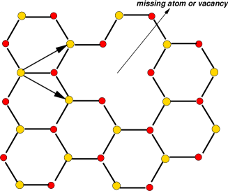
Figure 1: (color on line) A honeycomb lattice with vacancies, showing its primitive vectors.

In what follows we use a tight-binding description for the $\pi$-orbitals of Carbon with a Hamiltonian given by:

$$H_{{\rm t.b.}} = -t\sum_{\langle i,j\rangle,\sigma}(a^{{\dagger}}_{i,\sigma}b_{j,\sigma}+{\rm h.c.})$$ (5)

$$+ t^{\prime}\sum_{\langle\langle i,j\rangle\rangle,\sigma}(a^{{\dagger}}_{i,\sigma}a_{j,\sigma}+b^{{\dagger}}_{i,\sigma}b_{j,\sigma}+{\rm h.c.})\,,$$

where $a^{{\dagger}}_{i,\sigma}$ ($a_{i,\sigma}$) creates (annihilates) and electron on site ${\bf R}_{i}$ with spin $\sigma$ ($\sigma=\uparrow,\downarrow$) on sub-lattice $A$ and $b^{{\dagger}}_{i,\sigma}$ ($b_{i,\sigma}$) creates (annihilates) and electron on site ${\bf R}_{i}$ with spin $\sigma$ ($\sigma=\uparrow,\downarrow$) on sub-lattice $B$. $t$ is the nearest neighbor ($\langle i,j\rangle$) hopping energy ($t\approx 2.7$ eV), and $t^{\prime}$ is the next-nearest neighbor ($\langle\langle i,j\rangle\rangle$) hopping energy ($t^{\prime}/t\approx 0.1$). We notice en passant that in earlier studies of graphite McClure (1957) it has been assumed that $t^{\prime}=0$. This assumption, however, is not warranted since there is overlap between Carbon $\pi$-orbitals in the same sub-lattice. In fact, we will show that $t^{\prime}$ plays an important role in graphene since it breaks the particle-hole symmetry and is responsible for various effects observed experimentally.

Translational symmetry is broken by the presence of disorder. Localized defects such as vacancies and impurities are included in the tight-biding description by the addition of a local energy term:

$$H_{{\rm imp.}}=\sum_{i,\sigma}V_{i}\left(a^{\dagger}_{i,\sigma}a_{i,\sigma}+b^{\dagger}_{i+\bm{\delta}_{3},\sigma}b_{i+\bm{\delta}_{3},\sigma}\right)\,,$$ (6)

where $V_{i}$ is a random potential at site ${\bf R}_{i}$. In momentum space we define:

$$a^{\dagger}_{i,\sigma}=\frac{1}{\sqrt{N_{A}}}\sum_{\bm{k}}e^{i\bm{k}\cdot\bm{R}_{i}}a^{\dagger}_{\bm{k},\sigma}\,,\hskip 5.69046ptb^{\dagger}_{i,\sigma}=\frac{1}{\sqrt{N_{B}}}\sum_{\bm{k}}e^{i\bm{k}\cdot\bm{R}_{i}}b^{\dagger}_{\bm{k},\sigma}\,,$$ (7)

where $N_{A}=N_{B}=N$, and the non-interacting Hamiltonian, $H_{1}=H_{{\rm t.b.}}+H_{{\rm imp.}}$, reads:

$$H_{1} = \sum_{\bm{k},\sigma}[\phi(\bm{k})a^{\dagger}_{\bm{k},\sigma}b_{\bm{k},\sigma}+\phi^{\ast}(\bm{k})b^{\dagger}_{\bm{k},\sigma}a_{\bm{k},\sigma}]$$ (8)

$$+ \sum_{\bm{k},\sigma}\tilde{\phi}(\bm{k})(a^{\dagger}_{\bm{k},\sigma}a_{\bm{k},\sigma}+b^{\dagger}_{\bm{k},\sigma}b_{\bm{k},\sigma})$$

$$+ \sum_{\bm{q},\bm{k},\sigma}V_{{\bf q}}[a^{\dagger}_{\bm{k}+\bm{q},\sigma}a_{\bm{k},\sigma}+b^{\dagger}_{\bm{k}+\bm{q},\sigma}b_{\bm{k},\sigma}]\,,$$

where

$$\phi(\bm{k}) = -t\sum_{i=1}^{3}e^{i{\bf k}\cdot{\bf\delta}_{i}}\,,$$

$${\tilde{\phi}}(\bm{k}) = t^{\prime}\sum_{i=1}^{6}e^{i{\bf k}\cdot{\bf n}_{i}}\,,$$ (9)

and $V_{{\bf q}}$ is the Fourier transform of the random potential due to impurities. Hamiltonian (8) is the starting point of our approach.

II.1 The single impurity problem and the T-matrix approximation

In the single impurity case one can write $V_{\bf q}=V/N$ where $V$ is the strength of the impurity potential. In what follows we use standard finite temperature Green’s function formalism Doniach and Sondheimer (1988); Bruus and Flesberg (2004). Because of the existence of two sub-lattices, the Green’s function can be written as a $2\times 2$ matrix:

$$\bm{G}_{\sigma}(\bm{k},{\bf p},\tau)=\left(\begin{array}[]{cc}G_{AA,\sigma}(\bm{k},{\bf p},\tau)&G_{AB,\sigma}(\bm{k},{\bf p},\tau)\\ G_{BA,\sigma}(\bm{k},{\bf p},\tau)&G_{BB,\sigma}(\bm{k},{\bf p},\tau)\end{array}\right)\,,$$ (12)

where

$$G_{AA,\sigma}(\bm{k},{\bf p},\tau) = -\langle{\cal T}a_{\bm{k},\sigma}(\tau)a_{\bm{p},\sigma}^{{\dagger}}(0)\rangle\,,$$

$$G_{AB,\sigma}(\bm{k},{\bf p},\tau) = -\langle{\cal T}a_{\bm{k},\sigma}(\tau)b_{\bm{p},\sigma}^{{\dagger}}(0)\rangle\,,$$

$$G_{BA,\sigma}(\bm{k},{\bf p},\tau) = -\langle{\cal T}b_{\bm{k},\sigma}(\tau)a_{\bm{p},\sigma}^{{\dagger}}(0)\rangle\,,$$

$$G_{BB,\sigma}(\bm{k},{\bf p},\tau) = -\langle{\cal T}b_{\bm{k},\sigma}(\tau)b_{\bm{p},\sigma}^{{\dagger}}(0)\rangle\,,$$ (13)

where $\tau$ is the “imaginary” time, and ${\cal T}$ is the time ordering operator.

For a single impurity the Green’s function can be written as $\bm{G}(\bm{k},{\bf p},\tau)=\delta_{\bm{k},\bm{p}}\bm{G}(\bm{k},\tau)$, where Doniach and Sondheimer (1988):

$$\bm{G}(\bm{k},\omega_{n})=\bm{G}^{0}(\bm{k},\omega_{n})+\bm{G}^{0}(\bm{k},\omega_{n})\bm{T}_{{\rm imp.}}(\omega_{n})\bm{G}^{0}(\bm{k},\omega_{n})\,,$$ (14)

where $\omega_{n}=2\pi T(n+1/2)$ is the fermionic Matsubara frequency, $\bm{G}^{0}(\bm{k},\omega_{n})$ is the propagator of the tight-binding Hamiltonian (5) and

$$\bm{T}_{{\rm imp.}}(\omega_{n})=\frac{V}{N}[\bm{1}-V\bar{\bm{G}}^{0}(\omega_{n})]^{-1}\,,$$ (15)

is the single impurity T-matrix, where:

$$\bar{\bm{G}}^{0}(\omega_{n})=\frac{1}{N}\sum_{\bm{k}}\bm{G}^{0}(\bm{k},\omega_{n})\,.$$ (16)

The above result is exact for a single impurity. For a finite but small density, $n_{i}=N_{i}/N$, of impurities, the Green’s function equation becomes:

$$\bm{G}(\bm{k},\omega_{n})=\bm{G}^{0}(\bm{k},\omega_{n})+\bm{G}^{0}(\bm{k},\omega_{n})\bm{T}(\omega_{n})\bm{G}(\bm{k},\omega_{n})\,,$$ (17)

which is valid up to first order in $n_{i}$, that is, it takes only into account the multiple scattering of the electrons by a single impurity. Equation (17) can be solved as:

$$\bm{G}(\bm{k},\omega_{n})=[[\bm{G}^{0}(\bm{k},\omega_{n})]^{-1}-\bm{T}(\omega_{n})]^{-1}\,,$$ (18)

where

$$\bm{T}(\omega_{n})=N_{i}\bm{T}_{{\rm imp.}}(\omega_{n})=Vn_{i}[\bm{1}-V\bar{\bm{G}}^{0}(\omega_{n})]^{-1}\,.$$ (19)

For vacancies we take $V\to\infty$ and (19) reduces to:

$$\bm{T}(\omega_{n})=-n_{i}[\bar{\bm{G}}^{0}(\omega_{n})]^{-1}\,.$$ (20)

It worth stressing that Eqs. (14) and (15) although similar in form to Eqs. (18) and (19) have a very different meaning. Whereas the first set applies to the single impurity problem, the latter set is the consequence of an assemble average over the impurity positions (see Sec. V for details on the averaging procedure in the context of Landau levels) with a re-summation procedure, corresponding to the FBA Bruus and Flesberg (2004).

II.2 The low-energy physics and the electronic density of states

The results of the previous subsection are entirely general, in the sense that no approximation for the band structure was made. Consider, for simplicity, the tight-binding Hamiltonian (5) in the case of $t^{\prime}=0$, that can be written, in momentum space, as:

$$H_{{\rm t.b.}}=\sum_{{\bf k},\sigma}[a^{{\dagger}}_{{\bf k},\sigma},b^{{\dagger}}_{{\bf k},\sigma}]\cdot\left[\begin{array}[]{cc}0&\phi({\bf k})\\ \phi^{*}({\bf k})&0\end{array}\right]\cdot\left[\begin{array}[]{c}a_{{\bf k},\sigma}\\ b_{{\bf k},\sigma}\end{array}\right]\,,$$ (25)

which can be diagonalized and produces the spectrum:

$$E_{\pm}({\bf k})=\pm|\phi({\bf k})|\,,$$ (26)

where the plus (minus) sign is related with the upper (lower) band. It is easy to show that the spectrum vanishes at the $K$ point in the Brillouin zone with wave-vector, ${\bf Q}=(2\pi/(3\sqrt{3}a),2\pi/(3a))$, and other five points in the Brillouin zone related by symmetry. In fact, it is easy to show that:

$$\phi({\bf Q}+{\bf p}) \simeq \frac{3}{2}tae^{i\pi/3}(p_{y}-ip_{x})$$ (27)

$$+ \frac{3}{8}ta^{2}e^{i\pi/3}(p_{x}^{2}-p_{y}^{2}-2ip_{x}p_{y})\,,$$

$$\frac{\phi({\bf Q}+{\bf p})}{|\phi({\bf Q}+{\bf p})|} = e^{i\delta({\bf Q}+{\bf p})}\approx e^{i\pi/3}\frac{(p_{y}-ip_{x})}{|{\bf p}|}\,,$$ (28)

where $\bm{p}$ ($p\ll Q$) is measured relatively to the $K$ point in Brillouin zone and we have defined $e^{i\delta(\bm{k})}=\phi(\bm{k})/|\phi(\bm{k})|$, for latter use. Using (27) in (26) we find:

$$E_{\pm}({\bf Q}+{\bf p})\simeq\pm\frac{3}{2}ta|\bm{p}|=\pm v_{F}|\bm{p}|\,,$$ (29)

for the electron’s dispersion. Eq. (29) is the dispersion of a relativistic particle with “light” velocity $v_{F}=3ta/2$, that is, a Dirac fermion. Hence, at low energies (energies much lower than the bandwidth), the effective description of the tight-binding problem reduces the 6 points in the Brillouin zone to 2 Dirac cones, each one of them associated with a different sublattice. The low energy description is valid as long as the characteristic momenta (energy) of the excitations is smaller than a cut-off, $k_{c}$ ($D=v_{F}k_{c}$), of the order of the inverse lattice spacing. In the spirit of a Debye model, where one conserves the total number of states in the Brillouin zone, we choose $k_{c}$ such that $\pi k_{c}^{2}=(2\pi)^{2}/A_{c}$, where $A_{c}=3\sqrt{3}a^{2}/2$ is the area of the hexagonal unit cell. Hence, eq.(29) is valid for $p\ll k_{c}$ and $E\ll D=k_{c}v_{F}$.

So far we have discussed the case of $t^{\prime}=0$. When $t^{\prime}\neq 0$ the problem can also be easily diagonalized and one finds that, close to the K point, the electron dispersion changes to:

$$E_{\pm}({\bf Q}+{\bf p})\approx-3t^{\prime}\pm v_{F}|{\bf p}|+\frac{9t^{\prime}a^{2}}{4}{\bf p}^{2}\,,$$ (30)

showing that $t^{\prime}$ does not change the Dirac physics but introduces an asymmetry between the upper and lower bands, that is, it breaks the particle-hole symmetry. Hence, $t^{\prime}$ affects only the intermediate to high energy behavior and preserves the low-energy physics. For many of the properties discussed in this section $t^{\prime}$ does not play an important role and will be dropped. Nevertheless, we will see later that in the presence of extended defects $t^{\prime}$ plays an important role and has to be introduced in order to provide a consistent physical picture of graphene.

For $t^{\prime}=0$ we find:

$${G}_{AA}(\omega_{n},{\bm{k}}) = \sum_{j=\pm 1}\frac{1/2}{i\omega_{n}-j|\phi(\bm{k})|}\,,$$ (31)

$${G}_{AB}(\omega_{n},{\bm{k}}) = \sum_{j=\pm 1}\frac{je^{i\delta(\bm{k})}/2}{i\omega_{n}-j|\phi(\bm{k})|}\,,$$ (32)

$${G}_{BA}(\omega_{n},\bm{k}) = \sum_{j=\pm 1}\frac{je^{-i\delta(\bm{k})}/2}{i\omega_{n}-j|\phi(\bm{k})|}\,,$$ (33)

$${G}_{BB}(\omega_{n},{\bm{k}}) = {G}_{AA}(\omega_{n},\bm{k})\,.$$ (34)

The expansion of the energy around the K point simplifies greatly the expressions in the calculation of the T-matrix, since they lead to simpler forms to Eqs. (31)-(34). For the case of vacancies, Eq.(20), it is easy to see that at low energies the T-matrix reads:

$$\bm{T}(\omega_{n})=-n_{i}[\bar{G}_{AA}^{0}(\omega_{n})]^{-1}\,\bm{I}\,,$$ (35)

where $\bm{I}$ a 2$\times$2 identity matrix, and

$$\bar{G}_{AA}^{0}(\omega_{n}) = \frac{1}{2N}\sum_{j=\pm 1,{\bf k}}\frac{1}{i\omega_{n}-j|\phi(\bm{k})|}$$ (36)

$$= \frac{1}{2\rho}\sum_{j=\pm 1}\int\frac{d^{2}k}{(2\pi)^{2}}\frac{1}{i\omega_{n}-jv_{F}k}$$

$$= \frac{1}{4\pi\rho}\int_{0}^{k_{c}}\frac{dk\,k}{i\omega_{n}-jv_{F}k}$$

$$= -\frac{1}{4\pi\rho v_{F}^{2}}\,\,i\omega_{n}\ln\left(D^{2}/\omega_{n}^{2}\right)\,,$$

where $\rho=S/V$ is the graphene planar density ($S$ is the area of the graphene layer). After a Wick rotation ($i\omega_{n}\to\omega+i0^{+}$) one finds:

$$\bar{G}^{0}_{AA}(\omega+i0^{+})=-F_{0}(\omega)-i\pi\rho_{0}(\omega)\,,$$ (37)

where,

$$F_{0}(\omega) = \frac{2\omega}{D^{2}}\ln\left(\frac{D}{|\omega|}\right)\,,$$ (38)

$$\rho_{0}(\omega) = \frac{|\omega|}{D^{2}}\,,$$ (39)

where we have used that $\rho=1/A_{c}=k_{c}^{2}/(4\pi)$, and hence $4\pi\rho v_{F}^{2}=D^{2}$. In the above equations we always assume $|\omega|\ll D$. Notice that $\rho_{0}(\omega)$ is simply the density of states of two-dimensional Dirac fermions.

II.2.1 A single vacancy

Assuming that a single unit cell has been diluted, we use Eqs. (14) and (15) to determine the correction to the Dirac fermion density of states. The actual density of states, $\rho(\omega)$, is given by:

$$\rho(\omega) = -\frac{1}{\pi}{\rm Im}\bar{G}_{AA}(\omega+i0^{+})$$ (40)

$$= \rho_{0}(\omega)-\frac{2/N}{D^{2}}\frac{\rho_{0}(\omega)}{F_{0}^{2}(\omega)+\pi^{2}\rho_{0}^{2}(\omega)}$$

$$\approx \rho_{0}(\omega)-\frac{2/N}{|\omega|\log^{2}(D/|\omega|)}\hskip 14.22636pt(\omega\rightarrow 0)\,,$$

indicating that the contribution of the vacancy to the density of states is singular in the low frequency regime. The contribution is negative because one has exactly one missing state associated with the vacancy. The electronic wave function around a single impurity was computed in Ref.[Pereira et al., 2005]. The result obtained here is identical to the one obtained in the dilution problem in Heisenberg antiferromagnets Chernyshev et al. (2001, 2002). The reason for this coincidence is easy to understand: the low energy excitations of an antiferromagnet in the ordered Néel phase are antiferromagnetic magnons with linear dispersion relation, that is, relativistic bosons with a “speed of light” given by the spin-wave velocity. Since we have been discussing a non-interacting problem, the statistics plays no role, and the effect of disorder is the same for relativistic bosons or fermions.

II.2.2 The full Born approximation (FBA)

The situation is clearly different if one has a finite density of vacancies. In this case we have to deal with Eqs. (18) and (19) corresponding to the FBA where all one-impurity scattering events have been considered. As before, the density of states is given by $\rho(\omega)=-{\rm Im}\bar{G}_{AA}(\omega+i0^{+})/\pi$ and it is possible, after some tedious algebra, to obtain an analytical expression for this quantity, given by:

$$\rho(\omega) = \frac{\rho_{0}(\omega)}{D^{2}}\frac{2n_{i}}{a(\omega)}\ln\left(\frac{D^{2}}{b^{2}(\omega)+c^{2}(\omega)}\right)$$ (41)

$$+ \frac{1}{\pi D^{2}}\sum_{\alpha=\pm 1}\frac{\alpha b(\omega)}{a(\omega)}\left[\arctan\left(\frac{a(\omega)D}{c}\right)\right.$$

$$+ \left.\arctan\left(\frac{\alpha b(\omega)}{c(\omega)}\right)\right]\,,$$

with

$$a(\omega) = F_{0}^{2}(\omega)+\pi^{2}\rho_{0}^{2}(\omega)\,,$$

$$b(\omega) = a(\omega)\omega-n_{i}F_{0}(\omega)\,,$$

$$c(\omega) = n_{i}\pi\rho_{0}(\omega)\,,$$ (42)

where $F_{0}(\omega)$ and $\rho_{0}(\omega)$ are defined in (38) and (39), respectively. A plot of Eq. (41) is given in Fig. 2 for two values of the impurity concentration $n_{i}$. Once again, the low energy behavior of $\rho(\omega)$ is the same found in the context of diluted antiferromagnets. Chernyshev et al. (2001, 2002) We remark that the dilution procedure introduces a low energy scale proportional to $Dn_{i}$, as can be seen from panel (c) in Fig. 2.

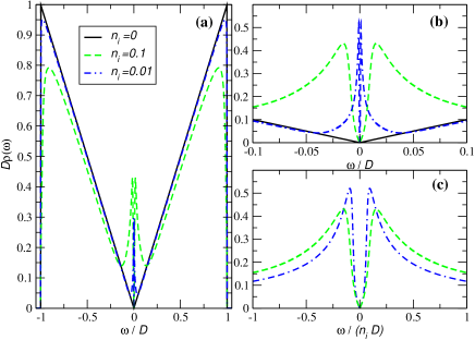
Figure 2: (color on line) Density of states obtained from the FBA. Panel (a) shows $\rho(\omega)$ over the entire band; panel (b) shows the low energy part, where it is seen that the peak in $\rho(\omega)$ has a higher value for lower $n_{i}$; panel (c) shows that the peak in $\rho(\omega)$ appears at an energy scale of the order of $n_{i}D/4$.

II.2.3 The full self-consistent Born approximation (FSBA)

The FBA does not take into account electronic scattering from multiple vacancies, it accounts only for multiple scattering from a single one. In order to include some contributions from multiple site scattering another partial series summation can be performed by replacing the bare propagator in the expression of the T-matrix in (20) by full propagator, leading to the FSBA. Because the matrix elements of the scattering potential computed from two Bloch states $|\bm{k}\rangle$ and $|\bm{p}\rangle$ are assumed momentum independent, the self-energy for the electrons depends only on the frequency. The self-consistent problem requires, in general, a careful numerical solution but in this particular case it is possible to reduce the problem to a set of coupled algebraic equations. The self-consistent problem requires the solution of the equation:

$$\Sigma(\omega_{n})=\frac{-n_{i}}{\bar{G}_{AA}^{0}(\omega_{n}-\Sigma(\omega_{n}))}\,,$$ (43)

where $\Sigma(\omega_{n})$ is the electron self-energy. One can show that the self-energy can be written as:

$$\Sigma(\omega+i0^{+})=\frac{n_{i}}{F(\omega)+i\pi\rho(\omega)}\,,$$ (44)

where $F(\omega)$ and $\rho(\omega)$ are determined by the following set of coupled algebraic equations:

$$F(\omega)=\frac{b}{2a(\omega)D^{2}}\Psi(F,\rho,\omega)+\frac{c(\omega)}{a(\omega)D^{2}}\Upsilon(F,\rho,\omega)\,,$$ (45)

$$\pi\rho(\omega)=\frac{c(\omega)}{2a(\omega)D^{2}}\Psi(F,\rho,\omega)-\frac{b(\omega)}{a(\omega)D^{2}}\Upsilon(F,\rho,\omega)\,,$$ (46)

where we used the definitions (42) and also defined the functions $\Psi(F,\rho,\omega)$ and $\Upsilon(F,\rho,\omega)$:

$$\Psi(F,\rho,\omega)\sum_{\alpha}\ln\left[\frac{(\alpha a(\omega)D+b(\omega))^{2}+c^{2}(\omega)}{b^{2}(\omega)+c^{2}(\omega)}\right]\,,$$ (47)

$$\Upsilon(F,\rho,\omega)=-2\arctan[b(\omega)/c(\omega)]$$

$$+\sum_{\alpha}\alpha\arctan[a(\omega)D/c(\omega)-\alpha b(\omega)/c(\omega)]\,.$$ (48)

The solution of Eqs. (45) and (46) describes the effect of the vacancies on the density of states of the Dirac Fermions. $\rho(\omega)$ is the self-consistent density of states, and $F(\omega)$ corresponds to the real part of self-energy (in analogy with $\rho_{0}(\omega)$ and $F_{0}(\omega)$ defined in (39) and (38)). In Fig. 3 we show the result of this procedure for various impurity concentrations.

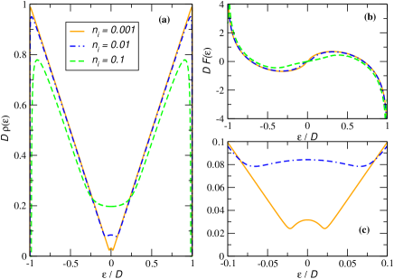
Figure 3: (color on line) Density of states obtained in FSBA. Panel (a) shows $\rho(\omega)$; panel (b) shows $F({\omega})$; panel (c) shows $\rho(\omega)$ at low energies.

The low-energy behavior of the density of states, showing a parabolic enhancement of $\rho(\omega)$, has also been found in the context of heavy-fermion superconductors Schmitt-Rink et al. (1986). An exact numerical calculation of the electronic density was carried out in Ref.[Pereira et al., 2005], where it was found that besides the low energy dome-like shape of the $\rho(\omega)$ (as shown in Fig. 3), a large peak appears very close to $\omega=0$. This peak is reminiscent of the single impurity result given in (40). Hence, besides the peak, the FSBA gives a very good account of the density of states in this problem.

Notice that the self-energy, $\Sigma(\omega)$, in (44) depends on $n_{i}$ in a non-trivial way, since both the self-consistent $F(\omega)$ and $\rho(\omega)$ also depend on $n_{i}$. The self-energy is depicted in Fig. 4 for various values of the dilution density $n_{i}$.

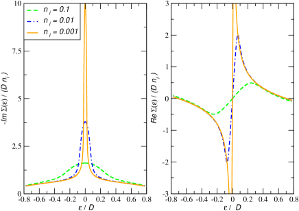
Figure 4: (color on line) Imaginary (left panel) and real (right panel) part of the self-energy obtained from the FSBA. Note that both quantities are divided by $Dn_{i}$.

III Spectral and transport properties

The electronic spectral function is defined as:

$$A(\bm{k},\omega)=-\frac{1}{\pi}{\rm Im}G(\bm{k},\omega+i0^{+})\,,$$ (49)

and can be interpreted as the probability density that an electron has momentum $\bm{k}$ and energy $\omega$. For a non-interacting, non-disordered, problem, the spectral function is simply a Dirac delta function at $\omega=E({\bf k})$. In the presence of disorder and/or electron-electron interactions the spectral function is broadened and its sharpness determines whether the electronic system supports quasi-particles. The spectral function can be measured directly in angle resolved photoemission experiments (ARPES) Zhou et al. (2005).

In terms of the self-energy, $\Sigma({\bf k},\omega)$, the spectral function reads:

$$A(\bm{k},\omega)=-\frac{1}{\pi}\frac{{\rm Im}\Sigma({\bf k},\omega)}{[\omega-E({\bf k})-{\rm Re}\Sigma({\bf k},\omega)]^{2}+[{\rm Im}\Sigma({\bf k},\omega)]^{2}}\,.$$ (50)

In the case of graphene, there are two contributions to the self-energy,

$$\Sigma({\bf k},\omega)=\Sigma_{{\rm e.-e.}}(\bm{k})+\Sigma_{{\rm dis.}}(\omega)\,,$$ (51)

where $\Sigma_{{\rm e.-e.}}(\bm{k})$ is the self-energy correction due to the electron-electron interactions that was computed originally in Ref. [González et al., 1992]:

$${\rm Im}\Sigma_{{\rm e.-e.}}(\bm{k})=\frac{1}{48}\left(\frac{e^{2}}{\epsilon_{0}v_{F}}\right)^{2}v_{F}|\bm{k}|\,,$$ (52)

where $e$ is the electron charge, and $\epsilon_{0}$ the dielectric constant of graphene. The other contribution, $\Sigma_{{\rm dis.}}$, is due to disorder and is given in (44).

Notice that these two contributions to the self-energy have very different dependence with the energy: while the electron-electron self-energy decreases as the energy (momentum) decreases, the self-energy due to disorder increases as the energy decreases. Hence, electron-electron interactions are dominant at high energies while disorder is dominant at low energies. This interplay between the two self-energies leads to the prediction that there will be a minimum in the self-energy for some energy where the electron-electron interaction becomes of the same order of the electron-vacancy interaction. In Fig. 5 we plot the self-energy as a function of energy for various impurity concentrations together with the spectral function (inset). One can clearly observe the non-monotonic dependence of the self-energy with the energy. This behavior should be observable in ARPES experiments.

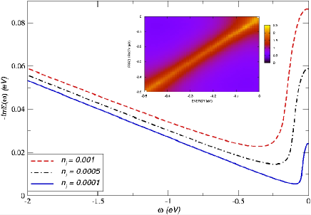
Figure 5: (color on line) Imaginary part of the electron’s self energy including both the effect of disordered and electron-electron interaction. The inset shows an intensity plot for the spectral function $A(\bm{k},\omega)$ for $D=8.248$ $eV$, $n_{i}=0.0001$.

Assuming an electric field applied in the $x$-direction, the frequency dependent (real part) conductivity is calculated from the Kubo formula:

$$\sigma({\bf q},\omega)=\frac{1}{\omega}\int_{0}^{\infty}dte^{i\omega t}\langle[J^{{\dagger}}_{x}({\bf q},t),J_{x}({\bf q},0)]\rangle$$ (53)

where $J_{x}$ is the $x$-component of the current operator which, due to gauge invariance, has the form Paul and Kotliar (2003):

$$J_{x}=-ite\sum_{i,\sigma,\bm{\delta}}\bm{u}_{x}\cdot\bm{\delta}a^{\dagger}_{i,\sigma}b_{i+\delta,\sigma}-\bm{u}_{x}\cdot\bm{\delta}b^{\dagger}_{i,\sigma+\delta}a_{i,\sigma}$$ (54)

(the notation $i+\delta$ means $\bm{R}_{i}+\bm{\delta}$). In Fourier space, and after expanding the general expression around the K-point in the Brillouin zone, we obtain:

$$J_{x}=-iv_{F}e\sum_{\bm{k},\sigma}(e^{-i\pi/3}a^{\dagger}_{\bm{k},\sigma}b_{\bm{k},\sigma}-e^{i\pi/3}b^{\dagger}_{\bm{k},\sigma}a_{\bm{k},\sigma})\,.$$ (55)

Substitution of (55) into (53) shows that the problem depends on the Green’s functions defined in (13). However, due to the special form of Eq. (28) the conductivity does not have contributions coming from products of Green’s functions of the form $G_{AB}G_{BA}$. Taking into account the number of bands and the spin degeneracy, the Kubo formula for the real part of the conductivity at finite frequency and temperature has the form:

$$\sigma(\omega,T)=-\frac{4v_{F}^{2}e^{2}}{NA_{c}\omega}\int_{-\infty}^{\infty}\frac{d\epsilon}{2\pi}[f(\epsilon+\omega)-f(\epsilon)]\times$$

$$\sum_{\bm{k}}{\rm Im}G_{AA}(\bm{k},\epsilon+i0^{+}){\rm Im}G_{AA}(\bm{k},\epsilon+\omega+i0^{+})\,,$$ (56)

where $f(\epsilon)=1/(e^{(\epsilon-\mu)/T}+1)$ is the Fermi-Dirac distribution function. The integral over $\bm{k}$ in (56) can be performed and find:

$$\sigma(\omega,T) = -\frac{e^{2}}{2\pi^{2}\omega}\int_{-\infty}^{\infty}d\epsilon[f(\epsilon+\omega)-f(\epsilon)]K(\omega,\epsilon)\,,$$ (57)

where

$$K(\omega,\epsilon)={\rm Im}\Sigma(\epsilon+\omega)\,\,{\rm Im}\Sigma(\epsilon)\,\,\Theta(\omega,\epsilon)\,,$$ (58)

($\Theta(\omega,\epsilon)$ defined in Appendix A).

It is instructive to consider the zero-temperature, zero-frequency limit of the conductivity in Eq. (56) (restoring $\hbar$):

$$\sigma_{0}=\frac{2}{\pi}\frac{e^{2}}{h}\left(1-\frac{[{\rm Im}\Sigma(0)]^{2}}{D^{2}+[{\rm Im}\Sigma(0)]^{2}}\right)\approx\frac{2}{\pi}\frac{e^{2}}{h}\,.$$ (59)

The result (59) shows that as long as ${\rm Im}\Sigma(0)\ll D$, $\sigma_{0}$ has a universal value independent of the dilution concentration, in agreement with earlier theoretical works Fradkin (1986); Lee (1993), and in agreement with the experimental data in graphene Novoselov et al. (2005a).

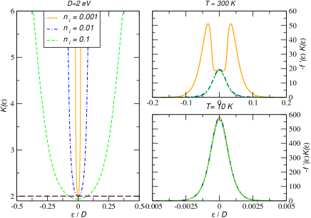
Figure 6: (color on line) Left: Kernel of the integral for $\sigma(0,T)$ as function of the energy. Product of the Fermi function derivative by $K(\epsilon)$ at two different temperatures.

At finite temperatures the integral in (57) has to be evaluated numerically. Consider $\sigma(0,T)$ whose behavior is determined by $K(\epsilon)\equiv K(0,\epsilon)$. The quantities $K(\epsilon)$ and $-f^{\prime}(\epsilon)K(\epsilon)$ ( $-f^{\prime}(\epsilon)$ is the derivative of the Fermi function in order to $\epsilon$) are both represented in Fig. 6. The behavior of $K(\epsilon)$ shows, “V”-like shape as the energy $\epsilon$ is varied. As a consequence, $\sigma(0,0)$ should present the same “V”-like shape as the chemical potential $\mu$ moves around $\mu=0$. Such behavior has indeed been observed in atomically thin carbon films Novoselov et al. (2004); Novoselov et al. (2005a), where the density of electrons was controled by a gate potential. The temperature dependence of the $\sigma(0,T)$, for $\mu=0$, is depicted in Fig. 7 for different vacancy concentrations, and it is found to follow Sommerfeld asymptotic expansion, but the number of terms needed to fit the numerical curve grows very fast as the dilution is reduced.

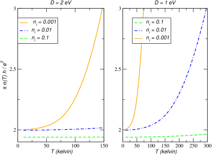
Figure 7: (color on line) Dependence of $\sigma(T,0)$ on the temperature and on the impurity dilution $n_{i}$.

In Fig. 8 we plot the frequency dependence of $\sigma(\omega,T)$ obtained from numerical integration of (57) with the self-energy given in (44). At low temperature, we see that $\sigma(\omega,T)$ develops a maximum around an energy value that is dependent on the number of impurities. In fact, if plot $\sigma(\omega,T)$ as function of $\omega/\sqrt{n_{i}}$, the conductivity almost shows scaling behavior for all impurity dilutions (see lower left panel). As the temperature increases, and if $\sigma(0,T)$ is sufficiently large, the conductivity $\sigma(\omega,T)$ acquires a Drude-like behavior (right panel).

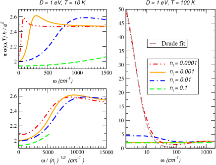
Figure 8: (color on line) Dependence of $\sigma(T,\omega)$ (in units of $e^{2}/(\pi\hbar)$) , on the frequency $\omega$.

IV Magnetic response and the role of short range Coulomb interactions

The ferromagnetism measured in proton irradiated graphite opens the question whether the interplay of interactions and disorder can drive the system from a paramagnetic to a magnetic ground state Esquinazi et al. (2003a). We study the effect of disorder on the magnetic susceptibility in the presence of short-range interactions, and the resulting change in the tendency towards magnetic instabilities. The problem of magnetic instabilities due to long-range exchange interactions Bloch (1929) in the presence of small density of carriers was discussed in great detail in ref. [Peres et al., 2005b]. We do not address here the effects associated to the interplay between the long-range Coulomb interaction and different types of lattice disorderStauber et al. (2005) and the appearance of local moments close to defects Ovchinnikov and Shamovsky (1991); Harigaya (2001); Lehtinen et al. (2004); Vozmediano et al. (2005).

The paramagnetic susceptibility of graphene is given by:

$$\chi(T) = \frac{\partial m_{z}}{\partial h}=4\frac{\partial}{\partial h}\frac{1}{N}\sum_{\bm{k}}\sum_{n}G_{AA}(\bm{k},i\omega_{n}-h)$$ (60)

$$= -4\int_{-\infty}^{\infty}d\epsilon f^{\prime}(\epsilon)\rho(\epsilon)\,,$$

where

$$m_{z}(T)=2\sum_{i,\sigma}\sigma\langle a^{\dagger}_{i,\sigma}a_{i,\sigma}\rangle\,,$$ (61)

is the magnetization, and $\rho(\epsilon)$ is the electronic density of states which, in the presence of disorder, is given in (46). Within the Stoner mechanism Stoner (1947), ferromagnetism is possible if the local electron-electron interaction term (the so-called Hubbard term)Tyutyulkov et al. (1998), $U$, is large than a critical value given by:

$$\frac{1}{U_{F}^{c}}=\frac{1}{4}\chi(0)\,.$$ (62)

In the case of an antiferromagnetic instability the same criteria would lead to another critical value of $U$ given by:

$$\frac{1}{U_{AF}^{c}}=\frac{2}{\pi D}\int_{-\infty}^{D}d\epsilon\rho(\epsilon)\arctan\left[\frac{D}{{\rm Im}\Sigma(\epsilon)}\right]\,.$$ (63)

Notice that in the case of antiferromagnetism one finds that $U_{AF}^{c}\approx D/(1-n_{i})$ when ${\rm Im}\Sigma\to 0$, in agreement with Hartree-Fock calculations Peres et al. (2004).

In Fig. 9 we plot the magnetic susceptibility as function of $T$ for different values of $n_{i}$. The signature of the presence of Dirac fermions comes from the linear dependence on $T$ for $T/D\ll 1$. Notice that, unlike the case of an ordinary metal that has a temperature dependent Pauli susceptibility, the graphene susceptibility increases with temperatures and number of impurities. At low temperatures $\chi(T)$ presents a small upturn not visible in Fig. 9. From the value of $\chi(0)$ and (62) we obtain the critical interaction required for a ferromagnetic transition, which is shown in the lower left panel of Fig. 9. Notice that the critical interaction strength for ferromagnetism decreases as the vacancy concentration increases indicating that disorder favors a ferromagnetic transition.

Using (63) and the results of the previous sections we can also calculate the critical value for an antiferromagnetic transition. The result is shown in the lower right panel of Fig. 9. In contrast with the ferromagnetic case, the antiferromagnetic instability is suppressed by disorder, requiring a large value of the electron-electron interaction. Notice that the value of the critical ferromagnetic coupling is always bigger than the antiferromagnetic one, indicating that at half-filling the graphene lattice is more susceptible to antiferromagnetic correlations. This result is consistent with an old proposal by Linus Pauling that graphene should be a resonant valence bond (RVB) state with local singlet correlations Pauling (1972).

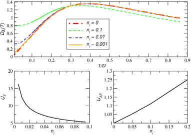
Figure 9: (color on line) Top: Dependence of $\chi(T)$ on the temperature and on the impurity dilution $n_{i}$. Bottom: Dependence of $U_{F}$ and $U_{AF}$ (in units of $D$) as function of $n_{i}$.

Hence, the Stoner criteria seems to be unable to explain the ferromagnetic behavior observed experimentally. One might ask whether additional scattering mechanisms, such that provided by long-range electron-electron interactions, can modify the critical values of the couplings. The self-energy correction due to long-range electron-electron scattering is given in (52) and can be added to the Dyson equation for the Green’s function and a new self-consistent density of states can be computed. This approach does not modify the value of $U_{F}^{c}$ which is determined by the low frequency behavior of the self-energy. In case of antiferromagnetism we find that indeed it leads to an increase on $U_{AF}^{c}$, but the result is non-conservative since the integral over the density of states gives a smaller value than $(1-n_{i})$. Therefore, we find from these calculations and previous ones Peres et al. (2005b) that graphene is not particularly susceptible to ferromagnetism.

V Magneto-Transport

The description of the magneto-transport properties of electrons in a disordered honeycomb lattice is complex because of the interference effects associated with the Hofstadter problem Gumbs and Fekete (1997). As in the previous sections, we simplify our problem by describing the electrons in the honeycomb lattice as Dirac fermions in the continuum. A similar approach was considered by Abrikosov in the quantum magnetoresistance study of non-stoichiometric chalcogenides Abrikosov (1998). In the case of graphene, the effective Hamiltonian describing Dirac fermions in a magnetic field (including disorder) can be written as: $H=H_{0}+H_{i}$ with

$$H_{0}=-v_{F}\sum_{i=x,y}\sigma_{i}[-i\partial_{i}+eA_{i}(\bm{r})]\,,$$ (64)

where, in the Landau gauge, $(A_{x},A_{y},A_{z})=(-By,0,0)$ is the vector potential for a constant magnetic field $B$ in the $z-$direction, $\sigma_{i}$ is the $i=x,y,z$ Pauli matrix, and

$$H_{i}=V{\sum_{j=1}^{N_{i}}\delta(\bm{r}-\bm{r}_{j})\bm{I}}\,.$$ (65)

The formulation of the problem in second quantization requires the solution of $H_{0}$, which is sketched in Appendix B. The field operators are defined as (see Appendix B for notation; the spin index is omitted for simplicity):

$$\Psi(\bm{r}) = \sum_{k}\frac{e^{ikx}}{\sqrt{L}}\left(\begin{array}[]{c}0\\ \phi_{0}(y)\end{array}\right)c_{k,-1}$$ (68)

$$+ \sum_{n,k,\alpha}\frac{e^{ikx}}{\sqrt{2L}}\left(\begin{array}[]{c}\phi_{n}(y-kl_{B}^{2})\\ \phi_{n+1}(y-kl_{B}^{2})\end{array}\right)c_{k,n,\alpha}\,.$$ (71)

The sum over $n=0,1,2,\ldots,$ is cut off at an $n_{0}$ given by $E(1,n_{0})=D$. In this representation $H_{0}$ becomes diagonal, leading to Green’s functions of the form (in Matsubara representation):

$$G_{0}(k,n,\alpha;i\omega)=\frac{1}{i\omega-E(\alpha,n)}\,,$$ (72)

is effectively $k$-independent, and $E(\alpha,-1)=0$ is the zero energy Landau level. The part of Hamiltonian due to the impurities is written as:

$$H_{i} = \frac{V}{L}\sum_{j=1}^{N_{i}}\sum_{p,k}e^{-ix_{j}(p-k)}\left[\phi_{0}(y_{j}-pl_{B}^{2})\phi_{0}(y_{j}-kl_{B}^{2})c^{\dagger}_{p,-1}c_{k,-1}+\sum_{n,\alpha}\frac{\alpha}{\sqrt{2}}\phi_{0}(y_{j}-pl_{B}^{2})\phi_{n+1}(y_{j}-kl_{B}^{2})c^{\dagger}_{p,-1}c_{k,n,\alpha}\right.$$ (73)

$$+ \sum_{n,\alpha}\frac{\alpha}{\sqrt{2}}\phi_{n+1}(y_{j}-pl_{B}^{2})\phi_{0}(y_{j}-kl_{B}^{2})c^{\dagger}_{p,n,\alpha}c_{k,-1}$$

$$+ \left.\sum_{n,m,\alpha,\lambda}\frac{1}{2}[\phi_{n}(y_{j}-pl_{B}^{2})\phi_{m}(y_{j}-kl_{B}^{2})+\alpha\lambda\phi_{n+1}(y_{j}-pl_{B}^{2})\phi_{m+1}(y_{j}-kl_{B}^{2})]c^{\dagger}_{p,n,\alpha}c_{k,m,\lambda}\right]\,.$$

Equation (73) describes the elastic scattering of electrons in Landau levels by the impurities. It is worth noting that this type of scattering connects Landau levels of negative and positive energy.

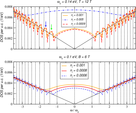
Figure 10: (color on line) Electronic density of states in a magnetic field for different dilutions and magnetic field. The non-disordered DOS and the position of the Landau levels in the absence of disorder are also shown. The two arrows in the upper panel show the position of the renormalized Landau levels (see Fig.11) given by the solution of Eq. (82). The energy is given in units of $\omega_{c}\equiv E(1,1)$.

V.1 The full self-consistent Born approximation

In order to describe the effect of impurity scattering on the magnetoresistance of graphene, the Green’s function for Landau levels in the presence of disorder needs to be computed. In the context of the 2D electron gas, an equivalent study was performed by Otha and Ando,Ohta (1968, 1971); Ato using the averaging procedure over impurity positions of DukeDuke (1968). Here the averaging procedure over impurity positions is performed in the standard way, namely, having determined the Green’s function for a given impurity configuration $(\bm{r}_{1},\ldots\bm{r}_{N_{i}})$, the position averaged Green’s function is determined from (as in Sec. II.1):

$$\langle G(p,n,\alpha;i\omega;\bm{r}_{1},\ldots\bm{r}_{N_{i}})\rangle\equiv G(p,n,\alpha;i\omega)$$

$$=L^{-2N_{i}}\left[\prod_{j=1}^{N_{i}}\int d\bm{r}_{j}\right]G(p,n,\alpha;i\omega;\bm{r}_{1},\ldots\bm{r}_{N_{i}})\,.$$ (74)

In Sec. II.1 the averaging involved plane wave states; in the presence of Landau levels the average over impurity positions involves the wave functions of the one-dimensional harmonic oscillator. In the averaging procedure we have used the following identities:

$$\int dy\phi_{n}(y-pl_{B}^{2})\phi_{m}(y-pl_{B}^{2}) = \delta_{n,m}\,,$$ (75)

$$\int dp\phi_{n}(y-pl_{B}^{2})\phi_{m}(y-pl_{B}^{2}) = \frac{\delta_{n,m}}{l^{2}_{B}}\,.$$ (76)

After a lengthy algebra, the Green’s function in the presence of vacancies, in the FSBA, can be written as:

$$G(p,n,\alpha;\omega+0^{+}) = [\omega-E(n,\alpha)-\Sigma_{1}(\omega)]^{-1}\,,$$ (77)

$$G(p,-1;\omega+0^{+}) = [\omega-\Sigma_{2}(\omega)]^{-1}\,,$$ (78)

where

$$\Sigma_{1}(\omega) = -n_{i}[Z(\omega)]^{-1}\,,$$ (79)

$$\Sigma_{2}(\omega) = -n_{i}[g_{c}G(p,-1;\omega+0^{+})/2+Z(\omega)]^{-1}\,,$$ (80)

$$Z(\omega) = g_{c}G(p,-1;\omega+0^{+})/2$$ (81)

$$+ g_{c}\sum_{n,\alpha}G(p,n,\alpha;\omega+0^{+})/2\,,$$

and $g_{c}=A_{c}/(2\pi l_{B}^{2})$ is the degeneracy of a Landau level per unit cell. One should notice that the Green’s functions do not depend upon $p$ explicitly. The self-consistent solution of Eqs. (77), (78), (79), (80) and (81) gives density of states, the electron self-energy, and the renormalization of Landau level energy position due to disorder.

The effect of dilution in the density of states of Dirac fermions in a magnetic field is shown in Fig. 10. For reference we note that $E(1,1)=0.14$ eV, for $B=14$ T, and $E(1,1)=0.1$ eV, for $B=6$ T. From Fig. 10 we see that given an impurity concentration the effect of broadening due to vacancies is less effective as the magnetic field increases. It is also clear that the position of Landau levels is renormalized relatively to the non-disordered case. The renormalization of the Landau level position can be determined from poles of (78):

$$\omega-E(\alpha,n)-{\rm Re}\Sigma(\omega)=0\,.$$ (82)

Of course, due to the importance of scattering at low energies, the solution to Eq. (82) does not represent exact eigenstates of system since the imaginary part of the self-energy is non-vanishing, however these energies do determine the form of the density of states, as we discuss below.

In Fig. 11, the graphical solution to Eq. (82) is given for two different energies ($E(-1,n)$, with $n=1,2$), being clear that the renormalization is important for the first Landau level. This result is due to the increase of the scattering at low energies, which is present already in the case of zero magnetic field. The values of $\omega$ satisfying Eq. (82) show up in density of states as the energy values where the oscillations due to the Landau level quantization have a maximum. In Fig. 10, the position of the renormalized Landau levels is shown in the upper panel (marked by two arrows), corresponding to the bare energies $E(-1,n)$, with $n=1,2$. The importance of this renormalization decreases with the reduction of number of vacancies. This is clear in Fig. 10 where a visible shift toward low energies is evident when $n_{i}$ has a small 10$\%$ change, from $n_{i}=10^{-3}$ to $n_{i}=9\times 10^{-4}$.

Figure 11: (color on line) Self-consistent results for $\Sigma_{1}(\omega)$ (top) and $\Sigma_{2}(\omega)$(bottom). The energy is given in units of $\omega_{c}\equiv E(1,1)$. In the left panels we show the intercept of $\omega-E(\alpha,n)$ with ${\rm Re}\Sigma(\omega)$ as required in (82).

V.2 Calculation of the transport properties

The study of the magnetoresistance properties of the system requires the calculation of the conductivity tensor. In terms of the field operators, the current density operator $\bm{j}$ is given by González et al. (1996):

$$\bm{j}=v_{F}e[\Psi^{\dagger}(x,y)\sigma_{x}\Psi(x,y),\Psi^{\dagger}(x,y)\sigma_{y}\Psi(x,y)]\,,$$ (83)

leading to current operator in the Landau basis written as:

$$J_{x} = v_{F}e\sum_{p,\alpha}\frac{1}{\sqrt{2}}\left[c^{\dagger}_{p,-1}c_{k,0,\alpha}+c^{\dagger}_{p,0,\alpha}c_{p,-1}\right]+v_{F}e\sum_{p,n,\alpha,\lambda}\frac{1}{2}\left[\lambda(1-\delta_{n,0})c^{\dagger}_{p,n,\alpha}c_{p,n-1,\lambda}+\alpha c^{\dagger}_{p,n,\alpha}c_{p,n+1,\lambda}\right]\,,$$ (84)

$$J_{y} = v_{F}e\sum_{p,\alpha}\frac{i}{\sqrt{2}}\left[c^{\dagger}_{p,-1}c_{k,0,\alpha}-c^{\dagger}_{p,0,\alpha}c_{p,-1}\right]+v_{F}e\sum_{p,n,\alpha,\lambda}\frac{i}{2}\left[-\lambda(1-\delta_{n,0})c^{\dagger}_{p,n,\alpha}c_{p,n-1,\lambda}+\alpha c^{\dagger}_{p,n,\alpha}c_{p,n+1,\lambda}\right]\,.$$ (85)

As in Sec. III, we compute the current-current correlation function and from it the conductivity tensor is derived. The diagonal component of the conductivity tensor $\sigma_{xx}(\omega,T)$ is given by (with the spin included):

$$\sigma_{xx}(\omega,T) = -\frac{4(v_{F}e)^{2}}{2\pi l_{B}^{2}}\frac{1}{\omega}\int_{-\infty}^{\infty}\frac{d\epsilon}{2\pi}[f(\epsilon+\omega)-f(\epsilon)]\left[\frac{1}{2}\sum_{\alpha_{1}}[{\rm Im}G(-1;\epsilon+i0^{+}){\rm Im}G(0,\alpha;\epsilon+\omega+i0^{+})\right.$$ (86)

$$+ {\rm Im}G(0,\alpha;\epsilon+i0^{+}){\rm Im}G(-1;\epsilon+\omega+i0^{+})]+\frac{1}{4}\sum_{n\geq 1,\alpha,\lambda}{\rm Im}G(n,\alpha;\epsilon+i0^{+}){\rm Im}G(n-1,\lambda;\epsilon+\omega+i0^{+})$$

$$+ \left.\frac{1}{4}\sum_{n\geq 0,\alpha,\lambda}{\rm Im}G(n,\alpha;\epsilon+i0^{+}){\rm Im}G(n+1,\lambda;\epsilon+\omega+i0^{+})\right]\,,$$

and the off-diagonal component $\sigma_{xy}(\omega,T)$ of the conductivity tensor is given by:

$$\sigma_{xy}(\omega,T) = \frac{2(v_{F}e)^{2}}{4\pi l_{B}^{2}}\frac{1}{\omega}\int_{-\infty}^{\infty}\frac{d\epsilon}{2\pi}\tanh\left(\frac{\epsilon}{2T}\right)\sum_{\alpha,\gamma}\left[\gamma[{\rm Re}G(0,\alpha;\epsilon+\gamma\omega+i0^{+}){\rm Im}G(-1;\epsilon+i0^{+})\right.$$ (87)

$$- {\rm Re}G(-1;\epsilon+\gamma\omega+i0^{+}){\rm Im}G(0,\alpha;\epsilon+i0^{+})]+\sum_{\lambda,n\geq 1}\frac{\gamma}{2}[{\rm Re}G(n,\alpha;\epsilon+\gamma\omega+i0^{+}){\rm Im}G(n-1,\lambda;\epsilon+i0^{+})$$

$$- \left.{\rm Re}G(n-1,\alpha;\epsilon+\gamma\omega+i0^{+}){\rm Im}G(n,\lambda;\epsilon+i0^{+})]\right]\,.$$

If we neglect the real part of the self-energy, and assume ${\rm Im}\Sigma_{i}(\omega)=\Gamma=$ constant ($i=1,2$), and let $\omega\to 0$, Eq. (86) reduces to Eq. (85) in Ref. [Gorbar et al., 2002], if we further assume the case $E(1,1)\gg\Gamma$ then Eq. (87) reduces to Eq. (86) of the same reference.

As in Sec. III, it is instructive to consider first the case $\omega,T\rightarrow 0$, which leads to ($\sigma_{xx}(0,0)=\sigma_{0}$):

$$\sigma_{0} = \frac{e^{2}}{h}\frac{2}{\pi}\left[\frac{{\rm Im}\Sigma_{1}(0)/{\rm Im}\Sigma_{2}(0)-1}{1+({\rm Im}\Sigma_{1}(0)/\omega_{c})^{2}}\right.$$ (88)

$$+ \left.\frac{n_{0}+1}{n_{0}+1+({\rm Im}\Sigma_{1}(0)/\omega_{c})^{2}}\right]\,.$$

When ${\rm Im}\Sigma_{1}(0)\simeq{\rm Im}\Sigma_{2}(0)$ and $\omega_{c}\gg{\rm Im}\Sigma_{1}(0)$ (or $n_{0}\gg{\rm Im}\Sigma_{1}(0)/\omega_{c}$), with $\omega_{c}=E(0,1)=\sqrt{2}v_{F}/l^{2}_{B}$, Eq. (88) reduces to: $\sigma_{0}\simeq 2/\pi(e^{2}/h)$, which is identical to the result (59) in the absence of the field found in Sec. III. This result was obtained previously by Ando and collaborators using the second order self-consistent Born approximation Shon and Ando (1998); Ando et al. (2002). However, in the FSBA it is required that the above conditions be satisfied for this result to hold. From Fig. 12 we see that the above conditions hold approximately over a wide ranges of field strength.

Figure 12: (color on line) Kernel of the conductivity (in units of $\pi h/e^{2}$) as function of energy for different magnetic fields and for a dilution concentration of $n_{i}=0.001$. The horizontal line represents the universal limit $\pi h\sigma_{0}/e^{2}=2$.

Because the d.c. magneto-transport properties have been measured graphene samples Novoselov et al. (2004) subjected to a gate potential (allowing to tune the electronic density), it is important to compute the conductivity kernel, since this has direct experimental relevance. In the the case $\omega\rightarrow 0$ we write the conductivity $\sigma_{xx}(0,T)$ as:

$$\sigma_{xx}(0,T)=\frac{e^{2}}{\pi h}\int_{-\infty}^{\infty}d\epsilon\frac{\partial f(\epsilon)}{\partial\epsilon}K_{B}(\epsilon)\,,$$ (89)

where the conductivity kernel $K_{B}(\epsilon)$ is given is Appendix A. The magnetic field dependence of kernel $K_{B}(\epsilon)$ is shown in Fig. 12. Observe that the effect of disorder is the creation of a region where $K_{B}(\epsilon)$ remains constant before it starts to increase in energy with superimposed oscillations coming from the Landau levels. The same effect, but with the absence of the oscillations, was identified at the level of the self-consistent density of states plotted in Fig. 10. Together with $\sigma_{xx}(0,T)$, the Hall conductivity $\sigma_{xy}(0,T)$ allows the calculation of the resistivity tensor:

$$\rho_{xx} = \frac{\sigma_{xx}}{\sigma_{xx}^{2}+\sigma_{xy}^{2}}\,,$$

$$\rho_{xy} = \frac{\sigma_{xy}}{\sigma_{xx}^{2}+\sigma_{xy}^{2}}\,.$$ (90)

Let us now focus on the optical conductivity, $\sigma_{xx}(\omega)$. This quantity can be probed by reflectivity experiments on the sub-THz to Mid-IR frequency range.Lin et al. (2005) We depict the behavior of Eq. (86) in Fig. 13 for different magnetic fields. It is clear that the first peak is controlled by the $E(1,1)-E(1,-1)$, and we have checked it does not obey any particular scaling form as function of $\omega/B$. On the other hand, as the effect of scattering becomes less important the high energy conductivity oscillations start obeying the scaling $\omega/\sqrt{B}$, as we show in the lower right panel of Fig. 13.

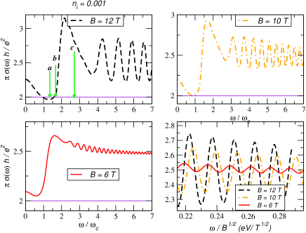
Figure 13: (color on line) Optical conductivity (in units of $\pi h/e^{2}$) at 10 $K$ as function of the energy for different magnetic fields and for a dilution concentration of $n_{i}=0.001$. The vertical arrows in the upper left panel, labeled a, b, and c, represent the renormalized $E(1,1)-E(-1,0)$, $E(2,1)-E(-1,0)$, and $E(1,1)-E(1,-1)$ transitions.

VI Extended defects

VI.1 Self-doping in the absence of electron-hole symmetry.

The standard description of a graphene sheet, following the usual treatment of the electronic band structure of graphiteBrandt et al. (1988); Slonczewski and Weiss (1958); McClure (1957); Dillon et al. (1977), assumes that in the absence of interlayer interactions the electronic structure of graphite shows electron-hole symmetry. This can be justified using a tight binding model by considering only hopping between $\pi$ orbitals located at nearest neighbor Carbon atoms. Within this approximation it can be shown that in certain graphene edgesWakayabashi and Sigrist (2000); Wakayabashi (2001) one would find a flat surface band Matsui et al. (2005). Disclinations (a pentagonal or heptagonal ring) can also lead to a discrete spectrum and states at zero energyGonzález et al. (1992, 1993). Other types of defects, like a combination of a five-fold and seven-fold ring (a lattice dislocation) or a Stone-Wales defect (made up of two pentagons and two heptagons) also lead to a finite density of states at the Fermi levelCharlier et al. (53); Matsumura and Ando (2001); Duplock et al. (2004).

Band structure calculations show that the electronic structure of a single graphene plane is not strictly symmetrical around the energy of the Dirac pointsReich et al. (2002). The absence of electron-hole symmetry shifts the energy of the states localized near impurities above or below the Fermi level, leading to a transfer of charge from/to the clean regions to the defects. Hence, the combination of localized defects and the lack of perfect electron-hole symmetry around the Dirac points leads to the possibility of self-doping, in addition to the usual scattering processes whose influence on the transport properties has been discussed in the preceding sections.

Point defects, like impurities and vacancies, can nucleate a few electronic states in their vicinity. Hence, a concentration of $n_{i}$ impurities per Carbon atom leads to a change in the electronic density of the regions between the impurities of order $n_{i}$. The corresponding shift in the Fermi energy is $\epsilon_{\rm F}\simeq v_{\rm F}\sqrt{n_{i}}$. In addition, the impurities lead to a finite elastic mean free path, $l_{\rm elas}\simeq an_{i}^{-1/2}$, and to an elastic scattering time $\tau_{\rm elas}\simeq(v_{\rm F}n_{i})^{-1}$, in agreement with the FSBA calculation in the preceding sections. Hence, the regions with few impurities can be considered low-density metals in the dirty limit, as $\tau_{\rm elas}^{-1}\simeq\epsilon_{\rm F}$.

Extended lattice defects, like edges, grain boundaries, or microcracks, are likely to induce the formation of a number of electronic states proportional to their length, $L/a$, where $a$ is of the order of the lattice constant. Hence, a distribution of extended defects of length $L$ at a distance proportional to $L$ itself gives rise to a concentration of $L/a$ carriers per unit Carbon in regions of order $(L/a)^{2}$. The resulting system can be considered a metal with a low density of carriers, $n_{\rm carrier}\propto a/L$ per unit cell, and an elastic mean free path $l_{\rm elas}\simeq L$. Then, we obtain:

$$\epsilon_{\rm F} \simeq \frac{v_{\rm F}}{\sqrt{aL}}$$

$$\frac{1}{\tau_{{\rm elas}}} \simeq \frac{v_{\rm F}}{L}$$ (91)

and, therefore, $(\tau_{{\rm elas}})^{-1}\ll\epsilon_{\rm F}$ when $a/L\ll 1$. Hence, the existence of extended defects leads to the possibility of self-doping but maintaining most of the sample in the clean limit. In this regime, coherent oscillations of the transport properties are to be expected, although the observed electronic properties will correspond to a shifted Fermi energy with respect to the nominally neutral defect–free system.

VI.2 Electronic structure near extended defects.

We describe the effects that break electron-hole symmetry near the Dirac points in terms of a finite next-nearest neighbor hopping between $\pi$ orbitals, $t^{\prime}$, in (5). From band structure calculationsReich et al. (2002), we expect that $|t^{\prime}/t|\leq 0.2$. We calculate the electronic structure of a ribbon of width $L$ terminated at zigzag edges, which are known to lead to surface states for $t^{\prime}=0$. The translational symmetry along the axis of the ribbon allows us to define bands in terms of the wavevector parallel to this axis. In Fig. 14, we show the bands closest to $\epsilon=0$ for a ribbon of width 200 unit cells and different values of $t^{\prime}/t$. The electronic structure associated to the interior region (the continuum cone), projected in Fig. 14 is not significantly changed by $t^{\prime}$. The localized surface bands, extending from $k_{\parallel}=(2\pi)/3$ to $k_{\parallel}=-(2\pi)/3$, on the other hand, acquires a dispersion of order $t^{\prime}$ (for a perturbative treatment of this effect, see ref. [Sasaki et al., 2005]). Hence, if the Fermi energy remains unchanged at the position of the Dirac points ($\epsilon_{\rm Dirac}=-3t^{\prime}$), this band will be filled, and the ribbon will no longer be charge neutral. In order to restore charge neutrality, the Fermi level needs to be shifted down (for the sign of $t^{\prime}$ chosen in the figure) by an amount of order $t^{\prime}$. As a consequence, some of the extended states near the Dirac points are filled, leading to the phenomenon of self-doping. The local charge as function of distance to the edges, setting the Fermi energy so that the ribbon is globally neutral. Note that the charge transferred to the surface states is very localized near the edges of the system.

Figure 14: Bands closest to the Dirac point of a graphene ribbon of 200 unit cells width. Top: $t^{\prime}=0$. Center: $t^{\prime}=-0.1t$. Bottom: $t^{\prime}=-0.2t$

Figure 15: Charge as function of the distance to the edge (in units of $a$) of a ribbon of width 300 $a$. Full line: $t^{\prime}/t=-0.2$. Broken line: $t^{\prime}/t=-0.1$. the Fermi energy is shifted upwards by $0.054t$ for $t^{\prime}=-0.1t$, and $0.077t$ for $t^{\prime}=-0.2t$.

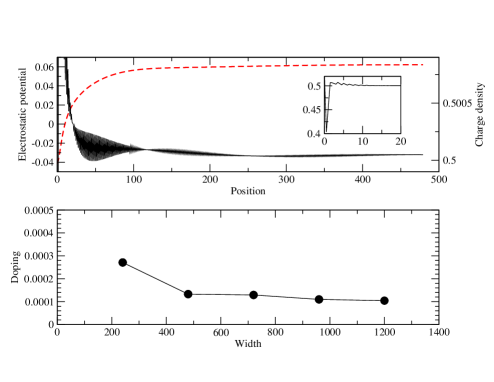
Figure 16: Top: Self-consistent charge density (continuous line) and electrostatic potential (dashed line) of a graphene ribbon with periodic boundary conditions along the zig-zag edge and with a circumference of size $W=80\sqrt{3}a$, and a length of $L=960a$. The parameters used are described in the text. The inset shows the details of the electronic density near the edge. Due to the presence of the edge, there is a displaced charge in the bulk (bottom panel) that is shown as a function of the width $W$.

VI.3 Electrostatic effects.

The charge transfer discussed in the preceding subsection is suppressed by electrostatic effects, as large deviations from charge neutrality have an associated energy cost. In order to study these charging effects we add to the free-electron Hamiltonian (5) the Coulomb energy of interaction between electrons:

$$H_{I}=\sum_{i,j}U_{i,j}n_{i}n_{j}\,,$$ (92)

where $n_{i}=\sum_{\sigma}(a^{{\dagger}}_{i,\sigma}a_{i,\sigma}+b^{{\dagger}}_{i,\sigma}b_{i,\sigma})$ is the number operator at site ${\bf R}_{i}$, and

$$U_{i,j}=\frac{e^{2}}{\epsilon_{0}|{\bf R}_{i}-{\bf R}_{j}|}\,,$$ (93)

is the Coulomb interaction between electrons. We expect, on physical grounds, that an electrostatic potential builds up at the edges, shifting the position of the surface states, and reducing the charge transferred to/from them. The potential at the edge induced by a constant doping $\delta$ per Carbon atom is roughly, $\sim(\delta e^{2}/a)(W/a)$ ($\delta e^{2}/a$ is the Coulomb energy per Carbon), and $W$ the width of the ribbon ($W/a$ is the number of Carbons involved). The charge transfer is arrested when the potential shifts the localized states to the Fermi energy, that is, when $t^{\prime}\approx(e^{2}/a)(W/a)\delta$. The resulting self-doping is therefore $\delta\sim(t^{\prime}a^{2})/(e^{2}W)$.

We treat the Hamiltonian (92) within the Hartree approximation (that is, we replace $H_{I}$ by $H_{{\rm M.F.}}=\sum_{i}V_{i}n_{i}$ where $V_{i}=\sum_{j}U_{i,j}\langle n_{j}\rangle$, and solve the problem self-consistently for $\langle n_{i}\rangle$). Numerical results for graphene ribbons of length $L=80\sqrt{3}a$ and different widths are shown in Fig. 15 and Fig. 16 ($t^{\prime}/t=0.2$ and $e^{2}/a=0.5t$). The largest width studied is $\sim 0.1\mu$m, and the total number of carbon atoms in the ribbon is $\approx 10^{5}$. Notice that as $W$ increases, the self-doping decreases indicating that, for a perfect graphene plane ($W\rightarrow\infty$), the self-doping effect disappears. For realistic parameters, we find that the amount of self-doping is $10^{-4}-10^{-5}$ electrons per unit cell for domains of sizes $0.1-1\mu$m, in agreement with the amount of charge observed in these systems.

Figure 17: Electronic levels of a graphene ribbon with zig-zag edges in the presence of a magnetic field ($t^{\prime}=-0.2t$). The magnetic flux per hexagon of the honeycomb lattice is $\Phi=0$ (top), $\Phi=0.00025$ (center), and $\Phi=0.0005$ (bottom), in units of the quantum of magnetic flux, $\Phi_{0}=h/e$. The corresponding magnetic fields are $0$T, $60$T and $120$T.

VI.4 Edge and surface states in the presence of a magnetic field.

We can analyze the electronic structure of a graphene ribbon of finite width in the presence of a magnetic field. The resulting tight binding equations can be considered as an extension of the Hofstadter problemHofstadter (1976) to a honeycomb lattice with edges. The bulk electronic structure is characterized by the Landau level structure discussed in previous sections. These states are modified at the edges, leading to chiral edge states, as discussed in relation to the Integer Hall Effect (IQHE)Halperin (1982). The existence of two Dirac points leads to two independent edge states, with the same chirality. In addition, Landau levels with positive energy should behave in an electron-like fashion, moving upwards in energy as their “center of gravity” approaches the edges. Landau levels with negative energy should be shifted towards lower energy near the edges.

A zig-zag edge induces also a non-chiral surface band. If the width of these states is much smaller than the magnetic field they will not be much affected by the presence of the field. The extension of the surface states is comparable to the lattice spacing for most of the range $|k_{\parallel}|\leq(2\pi)/3$, except near the Dirac points, so that the effect of realistic magnetic fields on these states is negligible.

The finite value of the second nearest neighbor hopping $t^{\prime}$ modifies the Landau levels obtained from the analysis of the Dirac equation. Elementary calculations (as those given in Appendix B) lead to:

$$E_{\pm}(n)=-3t^{\prime}+2l_{B}^{-2}\alpha\left(n+\frac{1}{2}\right)\pm\sqrt{l_{B}^{-4}\alpha^{2}+2l_{B}^{-2}\gamma^{2}n}\,,$$ (94)

with $n=0,1,2,3,\ldots$, $\alpha=9t^{\prime}a^{2}/4$ and $\gamma=3ta/2$, with the single assumption that $t\gg t^{\prime}$. This solution points out a number of interesting aspects, the most important of which is disappearance of the zero energy Landau level, made partially of holes and partially of electrons. With $t^{\prime}$, the electron or hole nature of the energy level becomes unambiguous, and half of the original zero energy Landau level (with $t^{\prime}=0$)moves down in energy (relatively to the Fermi energy) and the other half moves up. In addition, the level spacing for electron and hole levels becomes unequal.

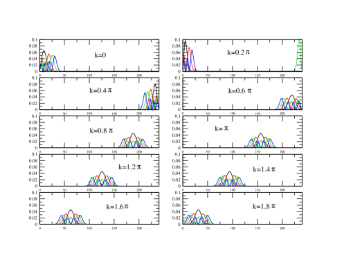
Figure 18: (Color online) Wave function of the lowest Landau levels for different momenta. Black: n=0. Red: n=1. Green: n=2. Blue: n=3.

The presence of a magnetic field acting on the ribbon does not break the translational symmetry along the direction parallel to the ribbon, that allows us to discuss the electronic structure in terms of the same bands calculated in the absence of the magnetic field. Results for the ribbon analyzed in Fig. 14 for different magnetic fields are shown in Fig. 17. The “center of gravity” of the wavefunctions associated to the levels moves in the direction transverse to the ribbon as the momentum is increased. The results show the bulk Landau levels, and their changes as the wavefunctions approach the edges. The surface band is practically unchanged, except for small avoided crossings every time that it becomes degenerate with a bulk Landau level. The results show quite accurately the expected scaling $\epsilon_{n}\propto\pm\sqrt{n}$ for the eigenenergies derived from the Dirac equation, with small corrections due to lattice effects and a finite $t^{\prime}$ (see Appendix B). The corresponding wavefunctions for different bands and momenta are shown in Fig. 18. The Landau levels move rigidly towards the edges, where one also find surface states.

We can compute the Hall conductivity from the number of chiral states induced by the field at the edgesHalperin (1982). If we fix the chemical potential above the $n$-th level, there are $2\times(2n+1)$ edge modes crossing the Fermi level (including the spin degeneracy). Hence, the Hall conductivity is:

$$\sigma_{xy}=\frac{e^{2}}{h}2\times(2n+1)=\frac{4e^{2}}{h}(n+1/2)\,.$$ (95)

This result should be compared with the usual IQHE in heterostructures, in which the factor of $1/2$ is absent. The presence of this $1/2$ factor is a direct consequence of the presence of the zero mode in the Dirac fermion problem. The existence of this anomalous IQHE was predicted long ago in the context of high energy physics Jackiw (1984); Schakel (1991) and more recently in the context of graphene Peres et al. (2005a); Gusynin and Sharapov (2005), but was observed in graphene only recently by two independent groups Novoselov et al. (2005a); Zhang et al. (2005c). An incomplete IQHE, with a finite longitudinal resistivity, was observed in HOPG graphite Kopelevich et al. (2003).

VI.5 Fractional quantum Hall effect

While the IQHE depends only of the cyclotron energy, $\omega_{c}$, and therefore is a robust effect, the fractional quantum Hall effect (FQHE) is a more delicate problem since it is a result of electron-electron interactions. The problem of electron-electron interactions in the presence of a large magnetic field in a honeycomb lattice is a complex problem that deserves a separate study. In this paper we make a few conjectures about the structure of the FQHE based on generic properties of Laughlin’s wave functions.

The electrons occupying the lowest Landau level are assumed to be in a many-body wavefunction written as (${\bf R}_{i}=(x_{i},y_{i})$ and $z=x+iy$) Murthy and Shankar (2003) :

$$\Psi=\exp(-i2m\sum_{i<j}\alpha_{i,j})\Phi(z_{1},\ldots,z_{N})\,,$$ (96)

where $\alpha_{i,j}=\arctan[{\rm Im}(z_{i}-z_{j})/{\rm Re}(z_{i}-z_{j})]$, $\Phi(z_{1},\ldots,z_{N})$ is an anti-symmetric function of the interchange of two $z^{\prime}s$, and $m=0,1,2,\ldots$. The effect of the singular phase associated with the many-body wave function is to introduce an effective magnetic field $B^{\ast}$ given by:

$$B^{\ast}=B-\bm{\nabla}\bm{a}(\bm{r})/e=B-2\pi(2m)\rho(\bm{r})/e\,,$$ (97)

where the gauge field $\bm{a}(\bm{r})$ is given by

$$\bm{a}(\bm{r}_{i})=2m\sum_{j\neq i}\bm{\nabla}(\bm{r}_{i})\alpha_{i,j}\,,$$ (98)

and $\rho(\bm{r})$ is the electronic density. The procedure outlined above is called flux-attachment and leads to appearance of composite fermions. These composite particles do not feel the external field $B$ but instead an effective field $B^{\ast}$. Therefore, the FQHE of electrons can be seen as an IQHE of these composite particles.

Given an electronic density $\delta$, we may define an effective filling factor $p^{\ast}$ for the composite particles as:

$$p^{\ast}=\frac{2\pi\delta}{eB^{\ast}}\,.$$ (99)

In the lowest Landau level the electron filling factor is:

$$p=\frac{2\pi\delta}{eB}\,,$$ (100)

and combining Eqs. (99) and (100) we obtain:

$$p=\frac{p^{\ast}}{2mp^{\ast}+1}\,,$$ (101)

so, we can write:

$$B^{\ast}=B(1-2mp)\,.$$ (102)

The crucial assumption in the case of graphene is that the effective $p^{\ast}$ associated with the integer quantum Hall effect of composite particles has the form given in (95), that is (spin ignored):

$$p^{\ast}=(2n+1)\,,\hskip 28.45274ptn=0,1,2,3,\ldots\,,$$ (103)

(the effective field $B^{\ast}$ is such that the system has one or more filled composite particle Landau levels, and the chemical potential lies between two these) leading to a quantized Hall conductivity given by:

$$\sigma_{xy}=\frac{2n+1}{2m(2n+1)+1}\frac{2e^{2}}{h}\,.$$ (104)

For $n=0$, one obtains the so-called Laughlin sequence: $\sigma_{xy}=1/(2m+1)(2e^{2}/h)$, and for $m=0$ we recover (95). This argument shows that Jain’s sequence is quite different from that of the 2D electrons gas Jain (1989).

As in the case of the IQHE, the FQHE can be thought in terms of chiral edge states, or chiral Luttinger liquids, that circulate at the edge of the sample Wen (1992). One can see the IQHE and FQHE as direct consequences of the presence of these edge states. Because of their chiral nature, edge states do not localize in the presence of disorder and hence the quantization of the Hall conductivity is robust. In graphene, as we have discussed previously, zig-zag edges support surface states that are non-chiral Luttinger liquids. We have recently shown that electron-electron interactions between chiral Luttinger liquids and non-chiral surface states can lead to instabilities of the chiral edge modes leading to edge reconstruction Castro Neto et al. (2005) and hence to the destruction of the quantization of conductivity. We also have shown that this edge reconstruction depends strongly on the amount of disorder at the edge of the sample. While this effect is not strong in the IQHE (because the cyclotron energy is very large when compared with the other energy scales), it makes the experimental observation of the FQHE in graphene very difficult.

VII Concluding Remarks

To summarize, we have analyzed the influence of local and extended lattice defects in the electronic properties of single graphene layer. Our results show that: (1) Point defects, such as vacancies, lead to an enhancement of the density of states at low energies and to a finite density of states at the Dirac point (in contrast to the clean case where the density of states vanishes); (2) Vacancies have a strong effect in the Dirac fermion self-energy leading to a very short quasi-particle lifetime at low energies; (3) The interplay between local defects and electron-electron interaction lead to the existence of a minimum in the imaginary part of the electron self-energy (a result that can be measured in ARPES); (4) The low temperature d.c. conductivity is a universal number, independent on the disorder concentration and magnetic field; (5) The d.c. conductivity, as in the case of a semiconductor, increases with temperature and chemical potential (a result that can be observed by applying a bias voltage to the system); (6) The a.c. conductivity increases with frequency at low frequency and at very low impurity concentrations can be fitted by a Drude-like model; (7) The magnetic susceptibility of graphene increases with temperature (it is not Pauli-like, as in an ordinary metal) and is sensitive to the amount of disorder in the system (it increases with disorder); (8) Within the Stoner criteria for magnetic instabilities we find that graphene is very stable against magnetic ordering and that the phase diagram of the system is dominated by paramagnetism; (9) In the presence of a magnetic field and disorder, the electronic density of states shows oscillations due to the presence of Landau levels which are shifted from their positions because of disorder; (10) The magneto-conductivity presents oscillations in the presence of fields and that their dependence with chemical potential and frequency are rather non-trivial, showing transitions between different Landau levels; (11) Extended defects, such as edges, lead to the effect of self-doping where charge is transfered from/to the defects to the bulk in the absence of particle-hole symmetry; (12) The effect of extended defects on transport is very weak and that electron scattering is dominated by local defects such as vacancies; (13) The quantization of the Hall conductance in the IQHE is anomalous relative to the case of the 2D electron gas with an extra factor of $1/2$ due to the presence of a zero mode in the Dirac fermion dispersion; (14) We conjecture that the FQHE in graphene has a sequence of states which is very different from the sequence found in the 2D electron gas and we propose a formula for that sequence.

The results and experimental predictions made in this work are based on a careful analysis of the problem of Dirac fermions in the presence of disorder, electron-electron interactions and external fields. We use well established theoretical techniques and find results that agree quite well with a series of amazing new experiments in graphene Novoselov et al. (2004); Berger et al. (2004); Zhang et al. (2005b); Novoselov et al. (2005a); Zhang et al. (2005a); Novoselov et al. (2005b); Zhang et al. (2005c). The main lesson of our work is that graphene presents a completely new electrodynamics when compared to ordinary metals which are described quite well within Landau’s Fermi liquid theory. In this work, we focus on the effects of disorder and electron-electron interaction and have shown that Dirac fermion respond to these perturbations in a way which is quite different from ordinary electrons. In fact, graphene is a non-Fermi liquid material where there is no concept of an effective mass and, therefore, a system where Fermi liquid concepts are not directly applicable. A new phenomenology, beyond Fermi liquid theory, has to be developed for this system. Our work can be considered a first step in that direction.

Appendix A $\Theta(\omega,\epsilon)$, and $K_{B}(\epsilon)$

In the calculation of $\sigma(\omega,T)$ and $\sigma(0,T)$ we defined:

$$\Theta(\omega,\epsilon) = \sum_{s_{1}=\pm 1,s_{2}=\pm 1}\left[\frac{N+s_{1}M}{B}\left(\arctan\left[\frac{D-s_{1}A}{B}\right]+\arctan\left[\frac{s_{1}A}{B}\right]\right)+\frac{P+s_{2}V}{E}\left(\arctan\left[\frac{D-s_{2}C}{E}\right]+\arctan\left[\frac{s_{2}C}{E}\right]\right)\right.$$ (105)

$$+ \left.\frac{M}{2}\log\left[\frac{(D-s_{1}A)^{2}+B^{2}}{A^{2}+B^{2}}\right]+\frac{V}{2}\log\left[\frac{(D-s_{1}C)^{2}+E^{2}}{C^{2}+E^{2}}\right]\right]\,,$$

where

$$M = (C^{2}+E^{2}-A^{2}-B^{2})/{\cal D},\hskip 14.22636ptV=-M\,,$$

$$N = 2(s_{1}A-s_{2}C)(A^{2}+B^{2})/{\cal D}\,,$$

$$P = -2(s_{1}A-s_{2}C)(A^{2}+B^{2})/{\cal D}\,,$$

$${\cal D} = (A^{2}+B^{2}-C^{2}-E^{2})^{2}\,$$

$$+ 4(A^{2}+B^{2})(C^{2}-s_{1}s_{2}AC)\,,$$

$$+ 4(C^{2}+E^{2})(A^{2}-s_{1}s_{2}AC)\,,$$

$$A = \epsilon+\omega-{\rm Re}\Sigma(\epsilon+\omega)\,,$$

$$B = {\rm Im}\Sigma(\epsilon+\omega)\,,$$

$$C = \epsilon-{\rm Re}\Sigma(\epsilon)\,,$$

$$E = {\rm Im}\Sigma(\epsilon)\,,$$

and $\cos\alpha=(C^{2}-E^{2})/(C^{2}+E^{2})$.

In the magneto-transport properties, $\sigma_{xx}(0,T)$ given by Eq. (89), depends on the kernel $K_{B}(x)$, which is defined as:

$$K_{B}(x) = \frac{v_{F}^{2}}{2\pi l_{B}^{2}}\sum_{\alpha}\left[\frac{{\rm Im}\Sigma_{2}(x)}{[x-{\rm Re}\Sigma_{2}(x)]^{2}+[{\rm Im}\Sigma_{2}(x)]^{2}}\frac{{\rm Im}\Sigma_{1}(x)}{[x-E(\alpha,0)-{\rm Re}\Sigma_{1}(x)]^{2}+[{\rm Im}\Sigma_{1}(x)]^{2}}\right.$$ (107)

$$+ \sum_{\lambda,n\geq 1}\left.\frac{{\rm Im}\Sigma_{1}(x)}{[x-E(\alpha,n)-{\rm Re}\Sigma_{1}(x)]^{2}+[{\rm Im}\Sigma_{1}(x)]^{2}}\frac{{\rm Im}\Sigma_{1}(x)}{[x-E(\lambda,n-1)-{\rm Re}\Sigma_{1}(x)]^{2}+[{\rm Im}\Sigma_{1}(x)]^{2}}\right]\,.$$

Appendix B The Dirac equation in a magnetic field

The Hamiltonian (64) can be solved using a trial spinor of the form:

$$\psi(\bm{r})\left(\begin{array}[]{c}c_{1}\phi_{1}(y)\\ c_{2}\phi_{2}(y)\end{array}\right)\frac{e^{ik_{x}x}}{\sqrt{L}}\,,$$ (108)

with $L$ the size of the system in the $x$ direction. After straightforward manipulations, the eigenproblem reduces to:

$${v_{F}\sqrt{2}}{l_{B}}\left(\begin{array}[]{cc}0&a\\ a^{\dagger}&0\end{array}\right)\left(\begin{array}[]{c}c_{1}\phi_{1}(y)\\ c_{2}\phi_{2}(y)\end{array}\right)E\left(\begin{array}[]{c}c_{1}\phi_{1}(y)\\ c_{2}\phi_{2}(y)\end{array}\right)\,,$$ (109)

where

$$a = \frac{1}{\sqrt{2}l_{B}}(y+l^{2}_{B}\partial_{y})\,,$$ (110)

$$a^{\dagger} = \frac{1}{\sqrt{2}l_{B}}(y-l^{2}_{B}\partial_{y})\,,$$ (111)

with the magnetic length defined as $l^{2}_{B}=1/(eB)$. For the case of $E\neq 0$, it is simple to see that the spinor

$$\frac{1}{\sqrt{2}}\left(\begin{array}[]{c}\phi_{n}(y)\\ \alpha\phi_{n+1}(y)\end{array}\right)\,,$$ (112)

is an eigenfunction of (109) with eigenvalue $E(\alpha,n)=\alpha v_{F}\sqrt{2}/l_{B}\sqrt{n+1}$, with $\alpha=\pm 1$, and $\phi_{n}$ ( $n=0,1,2,\ldots$) the $n$ eigenfunction of the usual 1D harmonic oscillator. In addition, there exists a zero energy mode whose eigenfunction is given by:

$$\left(\begin{array}[]{c}0\\ \phi_{0}(y)\end{array}\right)\,,$$ (113)

that completes the solution of the original eigenproblem. As in the more conventional Landau level problem, the degeneracy of each level is $L^{2}B/\phi_{0}$, with $\phi_{0}=h/e$ the quantum of flux.

References

- Brandt et al. (1988) N. B. Brandt, S. M. Chudinov, and Y. G. Ponomarev, in Modern Problems in Condensed Matter Sciences, edited by V. M. Agranovich and A. A. Maradudin (North Holland (Amsterdam), 1988), vol. 20.1.
- Rao et al. (2003) S. G. Rao, L. Huang, W. Setyawan, and S. H. Hong, Nature 425, 36 (2003).
- Sawamura et al. (2002) M. Sawamura, K. Kawai, Y. Matsuo, K. Kanie, T. Kato, and E. Nakamura, Nature 419, 702 (2002).
- Novoselov et al. (2004) K. S. Novoselov, A. K. Geim, S. V. Morozov, D. Jiang, Y. Zhang, S. V. Dubonos, I. V. Gregorieva, and A. A. Firsov, Science 306, 666 (2004).
- Berger et al. (2004) C. Berger, Z. M. Song, T. B. Li, X. B. Li, A. Y. Ogbazghi, R. Feng, Z. T. Dai, A. N. Marchenkov, E. H. Conrad, P. N. First, et al., J. Phys. Chem. B 108, 19912 (2004).
- Novoselov et al. (2005a) K. S. Novoselov, A. K. Geim, S. V. Morozov, D. Jiang, M. I. Katsnelson, I. V. Grigorieva, S. V. Dubonos, and A. A. Firsov, Nature 438, 197 (2005a).
- Novoselov et al. (2005b) K. S. Novoselov, D. Jiang, F. Schedin, T. J. Booth, V. V. Khotkevich, S. V. Morozov, and A. K. Geim, Proc. Nat. Acad. Sc. 102, 10451 (2005b).
- Zhang et al. (2005a) Y. Zhang, J. P. Small, M. E. S. Amori, and P. Kim, Phys. Rev. Lett. 94, 176803 (2005a).
- Bunch et al. (2005) J. S. Bunch, Y. Yaish, M. Brink, K. Bolotin, and P. L. McEuen, Nano Lett. 5, 2887 (2005).
- Zhang et al. (2005b) Y. Zhang, J. P. Small, W. V. Pontius, and P. Kim, Appl. Phys. Lett. 86, 073104 (2005b).
- Zhang et al. (2005c) Y. Zhang, Y.-W. Tan, H. L. Stormer, and P. Kim, Nature 438, 201 (2005c).
- Peres et al. (2005a) N. M. R. Peres, F. Guinea, and A. H. Castro Neto (2005a), eprint cond-mat/0506709.
- Castro Neto et al. (2005) A. H. Castro Neto, F. Guinea, and N. M. R. Peres (2005), eprint cond-mat/0509709.
- Gusynin and Sharapov (2005) V. P. Gusynin and S. G. Sharapov, Phys. Rev. Lett. 95, 146801 (2005).
- Esquinazi et al. (2003a) P. Esquinazi, D. Spemann, R. Höhne, A. Setzer, K.-H. Han, and T. Butz, Phys. Rev. Lett. 91, 227201 (2003a).
- Pauling (1972) L. Pauling, The Nature of the Chemical Bond (Cornell U. P., Ithaca, NY, 1972).
- DiVincenzo and Mele (1984) D. P. DiVincenzo and E. J. Mele, Phys.Rev.B 29, 1685 (1984).
- González et al. (1996) J. González, F. Guinea, and M. A. H. Vozmediano, Phys. Rev. Lett. 77, 3589 (1996).
- Mermin and Wagner (1966) N. D. Mermin and H. Wagner, Phys. Rev. Lett. 17, 1133 (1966).
- Davison and Sherrington (2000) L. Davison and D. Sherrington, J. Phys. A 33, 8615 (2000).
- Ritort and Sollich (2003) F. Ritort and P. Sollich, Adv. in Phys. 52, 219 (2003).
- Hashimoto et al. (2004) A. Hashimoto, K. Suenaga, A. Gloter, K. Urita, and S. Iijima, Nature 430, 870 (2004).
- r (1) See, for instance: P. J. Hirschfeld, and W. A. Atkinson, J. Low. Temp. Phys. 126, 881 (2002), and references therein.
- Kopelevich et al. (2000) Y. Kopelevich, P. Esquinazi, J. H. S. Torres, and S. Moehlecke, J. Low Temp. Phys. 119, 691 (2000).
- Esquinazi et al. (2002) P. Esquinazi, A. Setzer, R. Höhne, C. Semmelhack, Y. Kopelevich, D. Spemann, T. Butz, B. Kohlstrunk, and M. Lösch, Phys. Rev. B 66, 024429 (2002).
- Moehlecke et al. (2002) S. Moehlecke, P.-C. Ho, and M. B. Maple, Phil. Mag. Lett 82, 1335 (2002).
- Kempa et al. (2003) H. Kempa, H. C. Semmelhack, P. Esquinazi, and Y. Kopelevich, Solid State Commun. 125, 1 (2003).
- Esquinazi et al. (2003b) P. Esquinazi, D. Spemann, R. Höhne, A. Setzer, K.-H. Han, and T. Butz, Phys. Rev. Lett. 91, 227201 (2003b).
- Makarova and Palacio (2005) T. Makarova and F. Palacio, eds., Carbon-Based Magnetism: an overview of metal free carbon-based compounds and materials (Elsevier, Amsterdam, 2005).
- Peres et al. (2005b) N. M. R. Peres, F. Guinea, and A. H. Castro Neto, Phys. Rev. B 72, 174406 (2005b).
- McClure (1957) J. W. McClure, Phys. Rev. 108, 612 (1957).
- Doniach and Sondheimer (1988) S. Doniach and E. H. Sondheimer, Green’s functions for solid state physicists (World Scientific (Singapore), 1988).
- Bruus and Flesberg (2004) H. Bruus and K. Flesberg, Many-body Quantum Theory in Condensed Matter Physics (Oxford University Press, 2004).
- Pereira et al. (2005) V. M. Pereira, F. Guinea, J. M. B. L. dos Santos, N. M. R. Peres, and A. H. Castro Neto (2005), eprint cond-mat/0508530.
- Chernyshev et al. (2001) A. L. Chernyshev, Y. C. Chen, and A. H. Castro Neto, Phys. Rev. Lett. 87, 067209 (2001).
- Chernyshev et al. (2002) A. L. Chernyshev, Y. C. Chen, and A. H. Castro Neto, Phys. Rev. B 65, 104407 (2002).
- Schmitt-Rink et al. (1986) S. Schmitt-Rink, K. Miyake, and C. M. Varma, Phys. Rev. Lett. 57, 2575 (1986).
- Zhou et al. (2005) S. Y. Zhou, G.-H. Gweon, C. D. Spataru, J. Graf, D.-H. Lee, S. G. Louie, and A. Lanzara, Phys. Rev. B 71, 161403 (2005).
- González et al. (1992) J. González, F. Guinea, and M. A. H. Vozmediano, Phys. Rev. Lett. 69, 172 (1992).
- Paul and Kotliar (2003) I. Paul and G. Kotliar, Phys. Rev. B 67, 115131 (2003).
- Fradkin (1986) E. Fradkin, Phys. Rev. B 33, 3257 (1986).
- Lee (1993) P. A. Lee, Phys. Rev. Lett. 71, 1887 (1993).
- Bloch (1929) F. Bloch, Z. Physik 57, 549 (1929).
- Stauber et al. (2005) T. Stauber, F. Guinea, and M. A. H. Vozmediano, Phys. Rev. B 71, 041406 (2005).
- Ovchinnikov and Shamovsky (1991) A. A. Ovchinnikov and I. L. Shamovsky, Journ. of. Mol. Struc. (Theochem) 251, 133 (1991).
- Harigaya (2001) K. Harigaya, Journ. of Phys. C; Condens. Matt. 13, 1295 (2001).
- Lehtinen et al. (2004) P. O. Lehtinen, A. S. Foster, Y. Ma, A. V. Krasheninnikov, and R. M. Nieminen, Phys. Rev. Lett. 93, 187202 (2004).
- Vozmediano et al. (2005) M. A. H. Vozmediano, M. P. López-Sancho, T. Stauber, and F. Guinea, Phys. Rev. B 72, 155121 (2005).
- Stoner (1947) E. C. Stoner, Rep. Prog. Phys. 11, 43 (1947).
- Tyutyulkov et al. (1998) N. Tyutyulkov, G. Madjarova, F. Dietz, and K. Mullen, J. Phys. Chem. B 102, 10183 (1998).
- Peres et al. (2004) N. M. R. Peres, M. A. N. Araújo, and D. Bozi, Phys. Rev. B 70, 195122 (2004).
- Gumbs and Fekete (1997) G. Gumbs and P. Fekete, Phys. Rev B 56, 3787 (1997).
- Abrikosov (1998) A. A. Abrikosov, Phys. Rev B 58, 2788 (1998).
- Ohta (1968) K. Ohta, Japan. J. Appl. Phys. 10, 850 (1968).
- Ohta (1971) K. Ohta, J. Phys. Soc. Japan 31, 1627 (1971).
- (56) T. Ando and Y.Uemura, J. Phys. Soc. Japan 36, 959 (1974); T. Ando, J. Phys. Soc. Japan 36, 1521 (1974); ibidem 37, 622 (1974); ibidem 37, 1233 (1974); ibidem 38, 989 (1975).
- Duke (1968) C. B. Duke, Phys. Rev. 168, 816 (1968).
- Gorbar et al. (2002) E. V. Gorbar, V. P. Gusynin, V. A. Miransky, and I. A. Shovkovy, Phys. Rev. B 66, 045108 (2002).
- Shon and Ando (1998) N. H. Shon and T. Ando, J. Phys. Soc. Japan 67, 2421 (1998).
- Ando et al. (2002) T. Ando, Y. Zheng, and H. Suzuura, J. Phys. Soc. Japan 71, 1318 (2002).
- Lin et al. (2005) Z. Q. Lin, W. J. Padilla, S. V. Dordevic, K. S. Burch, Y. J. Wang, and D. N. Basov, unpublished (2005).
- Slonczewski and Weiss (1958) J. C. Slonczewski and P. R. Weiss, Phys. Rev. 109, 272 (1958).
- Dillon et al. (1977) R. O. Dillon, I. L. Spain, and J. W. McClure, J. Phys. Chem. Sol. 38, 635 (1977).
- Wakayabashi and Sigrist (2000) K. Wakayabashi and M. Sigrist, Phys. Rev. Lett. 84, 3390 (2000).
- Wakayabashi (2001) K. Wakayabashi, Phys. Rev. B 64, 125428 (2001).
- Matsui et al. (2005) T. Matsui, H. Kambara, Y. Niimi, K. Tagami, M. Tsukada, and H. Fukuyama, Phys. Rev. Lett. 94, 227201 (2005).
- González et al. (1993) J. González, F. Guinea, and M. A. H. Vozmediano, Nucl. Phys. B 406 [FS], 771 (1993).
- Charlier et al. (53) J. Charlier, T. W. Ebbesen, and P. Lambin, Phys. Rev. B 11108, 1996 (53).
- Matsumura and Ando (2001) H. Matsumura and T. Ando, J. Phys. Soc. Japan 70, 2657 (2001).
- Duplock et al. (2004) E. J. Duplock, M. Scheffler, and P. J. D. Lindan, Phys. Rev. Lett. 92, 225502 (2004).
- Reich et al. (2002) S. Reich, J. Maultzsch, C. Thomsen, and P. Ordejón, Phys. Rev. B 66, 035412 (2002).
- Sasaki et al. (2005) K. Sasaki, S. Murakami, and R. Saito (2005), eprint cond-mat/0508442.
- Hofstadter (1976) D. R. Hofstadter, Phys. Rev. B 14, 2239 (1976).
- Halperin (1982) B. I. Halperin, Phys. Rev. B 25, 2185 (1982).
- Jackiw (1984) R. Jackiw, Phys. Rev. D 29, 2375 (1984).
- Schakel (1991) A. M. J. Schakel, Phys. Rev. D 43, 1428 (1991).
- Kopelevich et al. (2003) Y. Kopelevich, J. H. S. Torres, R. R. da Silva, F. Mrowka, H. Kempa, and P. Esquinazi, Phys. Rev. Lett. 90, 156402 (2003).
- Murthy and Shankar (2003) G. Murthy and R. Shankar, Rev. Mod. Phys. 75, 1101 (2003).
- Jain (1989) J. K. Jain, Phys. Rev. Lett. 63, 199 (1989).
- Wen (1992) X.-G. Wen, Int. J. Mod. Phys. B 6, 1711 (1992).