Photoemission Beyond the Sudden Approximation

Abstract

The many-body theory of photoemission in solids is reviewed with emphasis on methods based on response theory. The classification of diagrams into loss and no-loss diagrams is discussed and related to Keldysh path-ordering book-keeping. Some new results on energy losses in valence-electron photoemission from free-electron-like metal surfaces are presented. A way to group diagrams is presented in which spectral intensities acquire a Golden-Rule-like form which guarantees positiveness. This way of regrouping should be useful also in other problems involving spectral intensities, such as the problem of improving the one-electron spectral function away from the quasiparticle peak.

1 Introduction

Photoemission spectroscopy[1] (PES) is since long a major tool for gaining information of the electronic structure of matter. For instance, angular resolved photoemission spectroscopy (ARPES) makes it possible to measure the occupied quasiparticle bands, and photoemission from core levels yields important local information at the atom being excited. Owing to the usually rather short mean free path, PES is also well suited for studying surface states, adsorbates at surfaces, etc.

Photoelectron spectra are usually interpreted in terms of the one-electron spectral function $A(\epsilon)$ corresponding to a sudden removal of an electron. In emission from solids, however, the photoelectron is created at a certain distance from the surface and may undergo losses on its way out. In the sixties, Berglund and Spicer[2] proposed a semi-empirical model involving primary excitation, transport to the surface, and transmission through the surfaces as three separate steps. Clearly a three-step description can at best be an approximation. An important step forward was taken by Schaich and Ashcroft[3] and by Mahan[4], who formulated the problem as a one-step quantum-mechanical process and presented model results for independent electrons. The Schaich-Ashcroft response formulation was soon generalized to account for interaction by Caroli et al.[5] who applied the formalism to phonon effects. Among important early works I would also like to mention the studies of plasmon losses by Langreth and collaborators [6, 7, 8, 9]. In particular, they explain why the satellites are greatly modified and suppressed also when the excitation energy is quite high, and why the satellites are so weak in, say, x-ray emission.

In strict one-electron theory, the photoelectrons cannot undergo losses by scattering against other electrons, phonons, and impurities. As a consequence, the entire solid will contribute to the photocurrent which is then limited by the penetration depth of the electromagnetic radiation. In reality, the current is limited by the escape depth of the photoelectrons, in practice usually just a few atomic layers. Thus the mean free path must somehow enter the theory, and in the mid-seventies ways to remedy this shortcoming were developed by Feibelman and Eastman[10], Pendry[11], and Liebsch[12, 13]. In essence, the no-loss photocurrent is to be calculated in a one-step but independent-electron way with one important exception: The photoelectron is assumed to move in the non-Hermitian optical potential, the (advanced) self-energy $\Sigma_{a}$. The photoelectron orbitals then get damped inside the sample, and the yield becomes limited by the photoelectron escape depth as it should. Today there exists several computer codes based on these ideas which take the underlying bandstructure into account in a realistic way.

The crucial point of introducing damped photoelectron orbitals was first obtained by Langreth[9] in the case of impurity scattering, and by Caroli et al.[5] in the case when the escape depth is limited by phonons. In the mid-eighties, by Almbladh[14] and Bardyszewski and Hedin [15] considered the problem of interacting electrons using two seemingly rather different techniques, one based on many-body perturbation theory and one based on scattering theory. These works largely justify the above one-electron-like methods for the no-loss photocurrent but they also predict corrections, which, for instance, modify the optical matrix elements.

There are several excellent recent reviews of solid-state photoemission [16, 17, 18]. In this paper, I would like to concentrate on how the techniques of non-equilibrium Green’s functions can be used both for obtaining approximations suitable for calculations in real materials as well as for obtaining general results like the structure of the quasiparticle no-loss part of a photoelectron spectrum.

2 Basic theory

I begin by a brief account of the quantum-mechanical description of the steady photoelectron current. As mentioned above, methods based on scattering theory[19, 4, 15], and methods based on quadratic response formalism and many-body perturbation theory[3, 5, 20, 6, 9, 14]. I begin by one-particle theory in order to illustrate the various limiting procedures, and generalize then to interacting systems.

2.1 Independent particles

Let us first consider independent electrons. The photoemission process can be considered as an inelastic scattering process with a photon in the initial state and an asymptotically free electron in the final state. In order to strengthen the analogy with scattering, let us take the system to occupy an finite volume $v$ enclosed in a quantization box of volume $V$. Because the photoelectron enters in the final rather than the initial state, its wavefunctions will obey ingoing wave boundary conditions[21, 19]. To first order in the radiative coupling we obtain

$$J_{p}=2\pi\sum_{n}^{occ}|\langle\chi_{p}^{-}|\Delta|n\rangle|^{2}\delta(\epsilon_{p}-\omega-\epsilon_{n}).$$ (1)

Here, $J_{p}$ is the momentum-decomposed photocurrent, $\Delta$ the coupling to the radiation field (cf. Eq. (5)), $\omega$ the photon energy, and $\epsilon_{\nu}$ one-electron energies. Atomic (Hartree) units are used.

The photoelectron spectrum probes the occupied part of the one-electron spectrum. For independent electrons, the spectral function can be written

$$A(\epsilon)=\sum_{n}|\phi_{n}\rangle\delta(\epsilon-\epsilon_{n})\langle\phi_{n}|$$ (2)

in terms of eigen-orbitals $\phi_{n}$. In terms of the spectral function, we have

$$J_{p}=2\pi\langle\chi_{p}^{-}|\Delta A(\epsilon_{p}-\omega)\Delta^{\dagger}|\chi_{p}^{-}\rangle$$ (3)

for photoelectron energies below threshold $\mu+\omega$. Here $\mu$ is the Fermi level relative to the vacuum level.

In order to compare with the response formulation of Schaich and Ashcroft, let us introduce orbitals $\phi_{\tilde{p}}$ which are plane waves well outside the sample and which vanish inside, and let $c_{\tilde{p}}$ be the associated destruction operator. We assume that the external field has been slowly switched on in the remote past, (modulated by $e^{\eta t}$), and take the average $2\eta\langle c_{\tilde{p}}^{+}c_{\tilde{p}}\rangle$ as a measure of the steady momentum-decomposed photocurrent. The details how the plane waves are truncated inside and near the sample will not influence the final results. We have

$$K(t)=H+\left[\delta He^{-i\omega t}+\delta H^{\dagger}e^{i\omega t}\right]e^{\eta t},$$ (4)

where $H$ describes the system in the absence of external fields, and where

$$\delta H=-\int{\mathbf{j}}({\mathbf{r}})\cdot{\mathbf{A}}({\mathbf{r}})=\sum_{kl}c_{k}^{+}c_{l}\Delta_{kl}$$ (5)

gives the coupling to the radiation field. We use a radiation gauge such that the scalar potential $\delta\Phi$ vanishes. (The diamagnetic coupling then gives no contribution to leading order, see Ref [3].) We assume that the system has been subject to the field for $t<0$, and define the photocurrent by

$$J_{p}=\lim_{\eta\rightarrow 0^{+}}2\eta\langle c^{+}_{\tilde{p}}c_{\tilde{p}}\rangle.$$ (6)

As in scattering theory the infinite volume limit should be taken before the limit $\eta\rightarrow 0$ , i.e., $\eta$ should be considered large compared to the level spacing due to the quantisation box V. Following Liebsch[12], we develop each initial-state orbital $n$ in time to obtain

$$\phi_{n,\eta}(t=0)=\left[1+G^{r}(\epsilon_{n}+\omega+i\eta)\Delta+G^{r}(\epsilon_{n}-\omega+i\eta)\Delta^{\dagger}\right]\phi_{n},$$ (7)

where $G^{r/a}(\epsilon)=1/(\epsilon-h\pm i\delta)$ are the retarded/advanced one-electron Green’s functions, and $h_{kl}$ the one-electron Hamiltonian matrix of the unperturbed system. We next form the expectation value $\langle c^{+}_{\tilde{p}}c_{\tilde{p}}\rangle$ and sum over occupied states initial states to obtain

$$J_{p} = \lim 2\eta\sum_{n}^{occ}|\langle\tilde{p}|G^{r}(\epsilon_{n}+\omega+i\eta)\Delta|n\rangle|^{2}$$ (8)

$$= \lim_{\eta\leftarrow 0}2\eta\int_{-\infty}^{0}dt\int_{-\infty}^{0}dt^{\prime}\;i\;\langle\tilde{p}|G^{r}(-t^{\prime})\Delta G^{<}(t^{\prime}-t)\Delta^{\dagger}G^{a}(t)|\tilde{p}\rangle\;e^{i\omega(t-t^{\prime})}\;e^{\eta(t+t^{\prime})}.$$ (9)

Here, $G^{<}$ is the usual lesser function, $\langle k|G^{<}(t)|l\rangle=i\langle N|c_{k}^{+}(0)c_{l}(t)|N\rangle$, and $|N\rangle$ the $N$-electron ground state. In order to obtain Eqs. (8, 9) we have used the fact that electrons in initial states $n$ are confined to the solid, and we have dropped the negative-frequency term which is easily seen not to contribute to the photocurrent in the limit $\eta\rightarrow 0^{+}$. In this limit one can further replace the truncated orbital $\phi_{\tilde{p}}$ with a plane wave $\phi_{p}$ (see e.g Ref. [14]). Eq. (9) is then equivalent to the Schaich-Ashcroft independent-electron result.

In order to see the equivalence between the scattering and response formulations, we express $G^{r/a}$ in terms of the Green’s function $G^{r/a}_{0}$ for free space and the scattering matrix $T^{r/a}$,

$$G^{r/a}(\epsilon)=G^{r/a}_{0}(\epsilon)+G^{r/a}_{0}(\epsilon)T^{r/a}(\epsilon)G^{r/a}_{0}(\epsilon).$$ (10)

As remarked above, we can replace the truncated plane wave $\phi_{\tilde{p}}$ with $\phi_{p}$ in the limit $V\rightarrow\infty$, $\eta\rightarrow 0^{+}$. In this limit we have

$$\langle n|1 + \Delta G^{a}(\epsilon_{n}+\omega-i\eta)|\tilde{p}\rangle=\langle n|\Delta G^{a}(\epsilon_{n}+\omega-i\eta)|\tilde{p}\rangle$$

$$= \frac{1}{\epsilon_{n}+\omega-\epsilon_{p}-i\eta}\langle n|\Delta[1+G^{a}_{0}(\epsilon_{p}-i\eta)T^{a}(\epsilon_{p}-i\eta)]|p\rangle$$

and the wave operator $1+G^{a}_{0}T^{a}$ transforms $\phi_{p}$ into $\chi^{-}_{p}$. In this way,

$$|\langle\tilde{p}|G^{r}(\epsilon_{n}+\omega+i\eta)\Delta|n\rangle|^{2}\rightarrow\frac{2\eta\langle\chi^{-}_{p}|\Delta|n\rangle|^{2}}{(\epsilon_{n}+\omega-\epsilon_{p})^{2}+\eta^{2}}\rightarrow 2\pi|\langle\chi^{-}_{p}|\Delta|n\rangle|^{2}\delta((\epsilon_{n}+\omega-\epsilon_{p}),$$

which establishes the equivalence between the response and the scattering approaches for independent electrons.

The geometry with a finite but possibly macroscopic sample is convenient for performing the somewhat subtle limits above, but in actual calculations one usually let the sample grow until it fills a half-space. The final-state orbitals $\chi^{-}_{p}$ are then replaced by their two-dimensional (2D) analogues, i.e., time-reversed states for scattering against the surface of the sample. These states are usually referred to as time-reversed LEED states because similar 2D scattering enters in the problem of low energy electron diffraction (LEED).

As stressed in the Introduction, strict one-particle theory is unphysical and leads to a yield limited by the radiation penetration depth rather than the photoelectron escape depth. If the propagators in Eq. (9) are replaced by their interacting counterparts, the final-state orbitals get damped inside the sample and the photocurrent limited by the escape depth as it should.

2.2 Interacting electrons

We expand $\langle c_{\tilde{p}}^{+}c_{\tilde{p}}\rangle$ directly in orders of the perturbation. The linear response vanishes identically because all electrons are confined to the sample in the ground state, $\tilde{c}^{+}_{p}\tilde{c}_{p}|N\rangle=0$. In the radiation gauge, the diamagnetic coupling involving ${\mathbf{A}}^{2}$ gives no contribution. The remaining contributions can be written

$$J_{p}(\epsilon)=\lim_{\eta\rightarrow 0^{+}}2\eta\int_{-\infty}^{0}dt\int_{-\infty}^{0}dt^{\prime}e^{i\omega(t-t^{\prime})}\;e^{\eta(t+t^{\prime})}\langle N|\delta H^{\dagger}(t)\hat{N}_{p}(0)\delta H(t^{\prime})|N\rangle.$$ (11)

Eq. (11) involves a three-particle path-ordered Green’s function

$$R_{p}(t,t^{\prime})=\sum_{klmn}\Delta^{*}_{k,n}\Delta_{l,m}\langle N|c^{+}_{k}(t)c_{n}(t)c^{+}_{\tilde{p}}(0)c_{\tilde{p}}(0)c^{+}_{l}(t^{\prime})c_{m}(t^{\prime})|N\rangle,$$ (12)

which may be evaluated by standard Keldysh technique[22]. To lowest order, all unconnected contractions vanish because

$$G^{<}(t)|\tilde{p}\rangle=0,\;\langle\tilde{p}|G^{<}(t)=0$$ (13)

both with and without interaction. By the same argument, there is only one non-vanishing connected contraction (see Fig. 1), which gives

$$R^{(0)}_{p}(t,t^{\prime}) = i\langle\tilde{p}|G^{>}_{0}(-t^{\prime})\Delta G^{<}_{0}(t-t^{\prime})\Delta^{\dagger}G^{>}_{0}(t)|\tilde{p}\rangle$$ (14)

$$= i\langle\tilde{p}|G^{r}_{0}(-t^{\prime})\Delta G^{<}_{0}(t-t^{\prime})\Delta^{\dagger}G^{a}_{0}(t)|\tilde{p}\rangle$$

when $t,\;t^{\prime}<0$. Eq. (14) gives back the previous independent-electron result in Eq. (9).

Figure 1: The lowest-order non-vanishing diagram for the photoemission process

In the present problem, the correlation $R_{p}(t,t^{\prime})$ in Eq. (12) is a ground-state correlation which simplifies the book-keeping of Keldysh diagrams. The Keldysh propagators refer to the contour in Fig. (2) which means that we assume that the interacting ground state can be generated by switching on the interaction adiabatically in the remote past,

$$R_{p}(t,t^{\prime})=\langle N,0|S^{\dagger}(\infty)\delta H^{\dagger}(t)c^{+}_{\tilde{p}}S(\infty)S^{\dagger}(\infty)c_{\tilde{p}}\delta H(t^{\prime})S(\infty)|N,0\rangle.$$ (15)

Thus $t=t_{-}$, $t^{\prime}=t^{\prime}_{+}$, and $c^{+}_{\tilde{p}}c_{\tilde{p}}$ is straddling the two branches of the Keldysh contour in Fig. (2). (The indices $\pm$ refer to the positive and negative time-ordered parts, respectively.) The propagators joining points $\mu,\;\nu$ of the different time-ordered parts are

$$G(t_{\mu},t_{\nu})=\begin{array}[]{l}G^{c}(t-t^{\prime}),\;\;\mu,\;\nu=+\\ G^{\tilde{c}}(t-t^{\prime}),\;\;\mu,\;\nu=-\\ G^{<}(t-t^{\prime}),\;\;\mu=+,\;\nu=-\\ G^{>}(t-t^{\prime}),\;\;\mu=-,\;\nu=+\;,\end{array}$$

where $G^{c}$, $G^{\tilde{c}}$ are propagators with positive and negative time-ordering, respectively, and $G^{\lessgtr}$ the usual lesser/greater functions. At zero temperature we have

$$a^{\lessgtr}(\epsilon)b^{\gtrless}(\epsilon)=0$$ (16)

for any Fermi propagators $a$ and $b$. Further, with the above assumption of adiabatic switching, the expansion of a time-ordered propagator will only involve propagators with the same time ordering.

Figure 2: Keldysh contour at $T=0$

The contribution from a general diagram can be reduced to a form analogous to the one-electron Golden Rule form in Eq. (1). In the expansion in full Green’s functions, any diagram ends with a pair of electron lines joined to the vertex $N_{p}$ representing the analyser (Fig. 3). This means that the correlation $R_{p}$ in Eq. (12) is of the general form

$$R_{p}(t,t^{\prime})=-\int\;dx\;d\tau\int\;dx^{\prime}\;d\tau^{\prime}\langle\tilde{p}|G^{c}(-\tau^{\prime})|x^{\prime}\rangle\langle x^{\prime}|I(t,t^{\prime};\tau,\tau^{\prime})|x\rangle\langle x|G^{\tilde{c}}(\tau)|\tilde{p}\rangle,$$ (17)

where $I$, the remain when the exit fermion lines have been removed, is invariant under a simultaneous translation of all four times and can be written

$$I(t,t^{\prime};\tau,\tau^{\prime})=\int\frac{d\nu d\nu^{\prime}d\nu^{\prime\prime}}{(2\pi)^{3}}I(\nu,\nu^{\prime};\nu^{\prime\prime},\nu^{\prime}+\nu^{\prime\prime}-\nu)\;e^{-i\nu t+i\nu^{\prime}t^{\prime}}e^{i\nu^{\prime\prime}\tau-(\nu+\nu^{\prime}-\nu^{\prime\prime})\tau^{\prime}}.$$ (18)

We notice that $G^{c}$ and $-G^{\tilde{c}}$ can be replaced by retarded and advanced propagators, respectively, since $\tilde{p}$ projects out the particle part. The action of $G^{r/a}$ on the orbitals $\tilde{p}$ and the limit $\eta\rightarrow 0$ can now be done analytically in much the same way as for independent particle, which gives

$$J_{p}=\langle\chi^{-}_{p}|I(\omega,\omega;\epsilon_{p},\epsilon_{p})|\chi^{-}_{p}\rangle.$$ (19)

Here $\chi^{-}_{p}$ is an one-electron time-reversed LEED orbital solved in the potential $V_{C}+\Sigma^{a}(\epsilon_{p})$. ($V_{C}$ is the total Coulomb potential from the nuclei and the equilibrium electron density.) The self-energy $\Sigma^{a}(\epsilon)$ is non-Hermitian with a finite imaginary part inside the sample. This makes $\chi^{-}_{p}$ decaying inside the sample with a decay length determined by energy losses. Thus all parts of the spectrum including the no-loss part is now limited by the escape depth of the photoelectrons.

Figure 3: Reduction of a general photoemission diagram

In the case of optical responses and transport, the ideas of self-consistent approximations put forward by Kadanoff and Baym[23, 24, 25] has been extremely successful. It is the present author’s opinion that this level in not possible to achieve in the case of photoemission. In particular, the Bethe-Salpeter equation which emerges as a result of selfconsistency will include interaction lines of all orders. If we open up such a diagram corresponding to a given approximation to the self-energy, infinitely many photoemission diagrams will result. For sp-bonded solids, the most important conserving approximation is the self-consistent screened exchange approximation[25, 26], usually referred to as the $GW$ approximation. Fortunately, the fulfilment of macroscopic conservation laws are less crucial for useful approximations to photoelectron spectra. In photoemission, only a small fraction of the emitted photoelectrons are actually measured. The majority of photoelectrons which make up the overall background is usually of no interest at all; instead the interest is focused on the spectral shapes in a limited energy window. Often, processes of different orders will contribute at different energies. Losses to plasmons is here a typical example. What is important is to have approximations which can explain the observed spectral profiles and which fulfil basic requirements such as positiveness.

2.3 Low-order diagrams

Let us expand the basic 3-particle correlation $R_{p}$ in orders of the screened interaction $W(\omega)=v\epsilon^{-1}(\omega)$. The non-vanishing first-order diagrams are shown in Fig. (4). As was the case for independent electrons, the condition in Eq. (13) limits the number of non-vanishing contractions. Vertices belonging to the forward (backward) time-ordered parts are are labelled + (-), respectively. The diagrams (a-c) involve only self-energy insertions and should be omitted if we expand in the full Green’s function. The remaining first-order diagrams fall into two classes, namely those with interaction line joining point in the same leg (d and e) and those with the interaction line joining points in different legs (f, g, and h). Consider first diagram f. It is well known that this diagram describes an extrinsic loss, but to illustrate the technique we give some details of the analysis. The interaction line here represents the boson-like correlation

$$W_{>}({\mathbf{r}}t,{\mathbf{r}}^{\prime}t^{\prime})=-i\langle N|\delta V_{H}({\mathbf{r}}t)\delta V_{H}({\mathbf{r}}^{\prime}t^{\prime})|N\rangle=-i\int_{0}^{\infty}\;d\omega^{\prime}B({\mathbf{r}},{\mathbf{r}}^{\prime},\omega^{\prime})e^{-i\omega^{\prime}(t-t^{\prime})},$$ (20)

where the spectral function $B$ is given by the dynamical structure factor $S({\mathbf{r}},{\mathbf{r}}^{\prime},\omega)$ convoluted with two Coulomb interactions ($v$), $B(\omega)=v*S(\omega)*v$. The fermion line from t’ to t represents $G^{<}$. and the remaining lines time-ordered or anti-time-ordered functions $G^{c/\tilde{c}}$. After reduction according to Eq. (19) we obtain

$$J_{p}^{(f)}=2\pi\int_{-\infty}^{0}d\epsilon\;\int_{0}^{\infty}\;d\omega^{\prime}\delta(\epsilon+\omega-\omega^{\prime}-\epsilon_{p})\langle\chi_{p}^{-}|\underbrace{G^{c}(\epsilon+\omega)\Delta A(\epsilon)\Delta^{\dagger}G^{c{\dagger}}(\epsilon+\omega)}_{B(\omega^{\prime})}|\chi_{p}^{-}\rangle$$ (21)

where we have used an underbrace to indicate how the spatial coordinates in $B(\omega)$ should be connected to the electron propagators. Here and in the following we use the identity $G^{\tilde{c}}(\epsilon)=-G^{c{\dagger}}(\epsilon)$ in order to express final results in spectral or lesser functions and functions with positive time-ordering.

The obvious physical interpretation of Eq. (21) is that it describes primary photo-excitation from an initial occupied level ($\epsilon$) to a level of energy $\epsilon+\omega$. The photoelectron then suffers an energy loss by exciting a plasmon or electron-hole pair of energy $\omega^{\prime}$ and hits the detector with an energy $\epsilon+\omega-\omega^{\prime}$. Consider next the diagrams g and h in Fig. 3. Using a similar technique as above we obtain

$$J_{p}^{(g)}+J_{p}^{(h)}=4\pi\Re\int_{-\infty}^{0}d\epsilon\;\int_{0}^{\infty}\;d\omega^{\prime}\delta(\epsilon+\omega-\omega^{\prime}-\epsilon_{p})\langle\chi_{p}^{-}|\underbrace{G^{c}(\epsilon+\omega)\Delta A(\epsilon)}_{B(\omega^{\prime})}G^{c{\dagger}}(\epsilon-\omega^{\prime})\Delta^{\dagger}|\chi_{p}^{-}\rangle$$ (22)

describing loss processes where interference between the potential from the hole left behind and the outgoing photoelectron interfere[7, 8, 9]. The ‘intrinsic’ losses, finally, are describe by the satellite structure of the hole spectral function A. The diagrams f-h plus the first-order satellite in $A$ ($c$) give the first-order contribution to the first plasmon satellite as obtained by Inglesfield[27] in the case of photoemission from core levels.

Figure 4: First-order diagrams for the photoemission process

We now turn to the first-order diagrams (d) and (e) with no interaction lines joining the (+) and (-) parts. In this case the interaction lines represent time-ordered correlations,

$$J_{p}^{(d)}=2\pi\int_{-\infty}^{0}d\epsilon\;\int_{0}^{\infty}\;d\omega^{\prime}\delta(\epsilon+\omega-\epsilon_{p})\langle\chi_{p}^{-}|\Lambda^{(1)}(\epsilon+\omega,\epsilon)A(\epsilon)\Delta^{\dagger}|\chi_{p}^{-}\rangle$$ (23)

where

$$\langle n|\Lambda^{(1)}(\epsilon,\epsilon^{\prime})|m\rangle=i\int\;\frac{d\omega^{\prime}}{2\pi}\langle n|\underbrace{G^{c}(\epsilon-\omega^{\prime})\Delta G^{c}(\epsilon^{\prime}-\omega^{\prime})}_{W^{c}(\omega^{\prime})}|m\rangle$$ (24)

is a first-order correction to the usual (time-ordered) vertex function. The diagram (e) gives the complex conjugate $[J_{p}^{(d)}]^{*}$. The appearance of $\delta(\epsilon+\omega-\epsilon_{p})$ in Eq. (23) shows that they contributes to the no-loss current.

The remaining two diagrams ($k$) and ($l$), finally, describe a screening of the photon field in the solid[10]. The screening will modify the electromagnetic field by local-field effects which are lattice-periodic deep inside the solid but more complicated near the surface. Most photoemission calculations to date do not take these effects into account. Effects of such screening has been considered by Liebsch[28], Schattke[29, 30], and by others. In the following discussion they will be considered included in the optical vertex $\Lambda$.

With independent-electron propagators, the photoelectron orbital is approximated to zeroth order in the interaction and is undamped inside the solid. If we regard the diagrams skeletons and use full Green’s functions (diagram ($c$) should then be omitted), the photoelectron orbital gets damped inside as it should.

2.4 Treatment based on scattering theory

Scattering theory furnishes an equivalent description of the photoemission process and has been the basis for several interesting new results[31, 32]. The obvious generalisation of the one-electron result is to replace the one-electron scattering orbital $|\chi^{-}_{p}\rangle$ by its many-body counterpart $|f\rangle\equiv|\chi^{-}_{p},s^{-}\rangle\equiv|N-1,s,p,-\rangle$ of energy $E_{f}=\epsilon_{p}+E_{s}(N-1)$ with an asymptotically free electron $p$ and a $N-1$-electron system left behind in some excited state $s$,

$$J_{p}=2\pi\sum_{s}|\langle f|\delta H|N\rangle|^{2}\delta(E_{i}-E_{f}))$$ (25)

The equivalence with the response formulation can be demonstrated with a variety of methods. One way is to consider the limiting behaviour of the amplitude

$$\langle N-1,s|c_{p}\delta H\frac{1}{E_{i}-H+i\eta}|N\rangle$$

inherent in the response formulation and verify that it tends to

$$\frac{1}{E_{i}-E_{f}+i\eta}\langle f|\delta H|N\rangle$$

when $\eta\rightarrow 0$. There are some subtleties involved because the photoelectron is identical the electrons in the sample. For a discussion, see e.g. Ref. [14].

A drawback with the above treatment is that every possible final many-body state has to be treated explicitly, a clearly impossible task in a ‘full’ treatment. In practice, however, one has so far only been able to account for losses to low orders. In sp-bonded materials, for example, the important excitations are boson-like and consist of plasmons and particle-hole pairs. The plasmons carry the major oscillator strength. Going back to Fig. (4), diagrams ($c$) and ($f-h$) all have a real boson in the final state. By summing over possible intermediate virtual states with some subspace, the propagators become renormalised and one obtains an approximation to the first boson loss satellite with damping properly included. The idea to work in subspaces is the essence of the Hedin-Bardyszewski approach[15]. To make the problem more clear-cut, Hedin following an idea of McMullen et al.[33] considered the photoelectron as distinguishable from other electrons in the sample, the ‘blue-electron model’.

The very existence of the Golden-Rule expression in Eq. (25) suggests that also the results from response theory can be put in a similar form. This is indeed the case, and a technique how it may be achieved will be discussed at the end of this paper.

3 No-loss current

Photoemission spectra typically consist of a quasi particle-like peak and various losses at lower kinetic energy. A mathematically precise definition of a no-loss part can only be given in the uninteresting case where the sample ends up in the $N-1$-particle ground state. If we are willing to accept a certain fuzziness, we can define a ”no-loss” part with about the same precision as quasi particles below the Fermi level. In practice there is usually no difficulty to identify, say, core-electron quasi particles, or valence-electron quasi particles well below the Fermi energy so long as their lifetime broadening is small on the energy scale of interest.

Our foregoing analysis suggest that interaction lines which join the positive and negative time-ordered parts of a diagram correspond to energy losses in the final state. There must always be at least one $G^{<}$ line joining the two optical vertices in a diagram, i.e, there is always an excitation where an electron has been removed. In first order, the diagrams ($c$, $f-h$) in Fig. (4) contribute to additional losses involving particle-hole pairs or plasmons because they involve $W^{>}$. In an interaction-picture representation for 3-current correlation $R_{p}$ we have

$$R_{p}(t,t^{\prime})=\langle 0|T^{\dagger}\left[S(-\infty,\infty)\delta H(t)c(0)\right]T\left[S(-\infty,\infty)c(0)\delta H(t)\right]|0\rangle.$$ (26)

We insert a complete set of final $N-1$-electron states between the forward- and backward time-ordered parts and expand. The $N-1$ electron ground state corresponds to ejecting an electron from the Fermi surface adiabatically. If the sample has well-defined quasi particles it is natural to filter out all final states with energies a couple of lifetime widths away for the quasi-particle energy. This corresponds essentially to excluding interaction and electron lines which cross the two time-ordering parts. If we sum all diagrams of this kind, we obtain

$$J_{p}=2\pi\;\int_{-\infty}^{\mu}\delta(\epsilon_{p}-\epsilon-\omega)\langle\chi_{p}^{-}|\Lambda(\epsilon+\omega,\epsilon)A(\epsilon)\Lambda^{\dagger}(\epsilon+\omega,\epsilon)|\chi_{p}^{-}\rangle\;d\epsilon$$ (27)

(see Fig (5)). Here, $\Lambda(\epsilon,\epsilon^{\prime})$ is the screened, time-ordered vector-coupling vertex. In order to obtain only the no-loss part the integration with respect to $\epsilon$ should be confined to the quasi particle part of $A(\epsilon)$. How this should be done cannot be specified exactly, as a consequence of the fact that the sample is generally left in an unstable excited state. The impreciseness is of the order of the lifetime width of the hole left behind. Experimental angular-resolved spectra show that the quasi-particle concept is useful also for states far below the Fermi energy and that spectra of real systems can be considered composed of a no-loss part that reflects the quasi-particle bandstructure, and a loss part that reflects the dynamical response of the system.

The vertex correction is clearly related to the problem of how the optical matrix elements should be calculated. In the dipole approximation, the velocity ($\Delta_{kl}\sim\langle k|{\mathbf{A}}\cdot{\mathbf{p}}|l\rangle$), length ($\Delta_{kl}\sim\langle k|{\mathbf{E}}\cdot{\mathbf{r}}|l\rangle$), and acceleration ($\Delta_{kl}\sim\langle k|A\cdot\nabla w({\mathbf{r}})|l\rangle$) formulas are equivalent. For independent particles the equivalence readily follows by commuting the one-electron Hamiltonian with the momentum, and $w$ is then the effective one-electron lattice potential. When the independent-electron propagators are replaced by their interacting counterparts, however, the equivalence is lost. There is also a question how the effective potential $w$ should be chosen. This problem resolved by the present author in the mid-eighties[34]. The replacement of the bare optical matrix element by the dressed vertex $\Lambda_{v/L/a}$ restores the equivalence almost completely[34]. The remaining discrepancy is of order of the lifetime width of the hole left behind and is clearly related to the fuzziness of quasi particles away from the Fermi surface. This again shows that Eq. (27) furnishes a good description in systems with well-defined quasi particles. The acceleration matrix elements involve $\epsilon^{-1}(\omega){\mathbf{A}}\cdot\nabla w_{nuc}({\mathbf{r}})$ (a polarisation where are nuclei have been shifted a distance ${\mathbf{A}}$. The last result was first obtained by Hermeking[20].

Figure 5: The no-loss part of the photocurrent

4 Energy Losses

We shall here mainly be concerned with plasmon losses in sp-bonded materials. As is well known plasmon losses can be produced either ”intrinsically” in connection with the primary photo-excitation, or ”extrinsically” by the escaping photoelectron on its way out. At lower kinetic energies the two modes of plasmon excitation interfere, leading to a suppression of the satellite strength. This interference has in the past been described using semi-classical models where the photoelectron is assumed to follow a classical trajectory and where the photoelectron and the hole left behind are represented by external potentials[35, 36, 37, 38]. In the case of core-electron photoemission, Hedin et al.[31, 39] have shown that a fully quantum-mechanical description of the leading satellites agrees quite well with a semi-classical description for excitation energies a couple of plasmon energies above threshold. It also shows that interference between intrinsic and extrinsic plasmon production persists up to the keV range, thereby confirming the earlier works by Chang and Langreth[7, 8]. However, there are to our knowledge no similar studies for photoemission from valence states.

As will be discussed below, a straight-forward expansion in orders of the screened interaction $W$ will not in general guarantee positive spectral densities. I will here outline a different summation order in which the partial sums have a golden-rule-like form involving transition amplitudes $\tau_{fi}$. Thus, each partial sum has the generic form

$$I(\omega)=\sum_{f}|\tau_{fi}|^{2}\delta(E_{i}+\omega-I_{f}),$$ (28)

where $i,f$ label real excitations in the initial and final states, respectively. The transition amplitudes can be related to cut Keldysh diagram. By performing an expansion of the amplitudes to a given order, each partial sum gives a positive result. The procedure amounts to splitting complete Keldysh diagrams in pieces and to sum them a particular order such that every partial sum is positive. If carried out of infinite order, ‘all’ complete diagrams are summed. I will outline the procedure with the low-order plasmon losses in photoemission as an example, and give some new model results for valence photoemission from a simple-metal surface.

4.1 Lowest-order contributions

Let us begin with the lowest-order contributions where no real losses have occurred. Up to first order in $W$, the zeroth-order diagram in Fig. 1 and diagrams (d) and (e) in Fig. 4 contribute and will involve the combination

$$\langle\chi_{p}^{-}|\Delta A(\epsilon)\Delta^{\dagger}|\chi_{p}^{-}\rangle+2\Re\langle\chi_{p}^{-}|\Lambda^{(1)}(\epsilon+\omega,\epsilon)\Delta A(\epsilon)\Delta^{\dagger}|\chi_{p}^{-}\rangle.$$

The obvious missing piece in the above approximation is the term $\langle\chi_{p}^{-}|\Lambda^{(1)}A(\epsilon)\Lambda^{(1){\dagger}}|\chi_{p}^{-}\rangle$. If this term is added, a manifestly positive result is obtained,

$$\langle\chi_{p}^{-}|[\Delta+\Lambda^{(1)}]A(\epsilon)[\Delta+\Lambda^{(1)}]^{\dagger}|\chi_{p}^{-}\rangle$$

in which the transition amplitudes rather than the spectral intensity has been truncated to a given order.

Contributions with no real excitations in the final state are somewhat artificial and will give no contribution when particle-hole excitations are included in the screened interaction. The mechanism is essentially the same as in the Langreth theorem[40]. In the case of the simpler $G^{<}$ function we have

$$G^{<}(\epsilon)=[1+G^{r}(\epsilon)\Sigma^{r}(\epsilon)]G_{0}^{<}(\epsilon)[1+\Sigma^{a}(\epsilon)G^{a}(\epsilon)]+G^{r}(\epsilon)\Sigma^{<}(\epsilon)G^{a}(\epsilon).$$ (29)

If there are no real excitations in a particular spectral region, $\Sigma^{<}$ vanishes, and the first term in Eq. (29) gives the entire contribution. As soon as real excitations occur, the first term tends to zero in the infinite-volume limit and the entire contribution comes from the second term. What actually occurs is that previously sharp single-particle-like excitations become broadened. By the same mechanism, contributions with no real excitations in the final state except a perfectly sharp quasi particle will not contribute to the photoemission current when broadening by particle-hole pairs is included.

We next proceed to the first-order diagrams $(c)$ and $(f-h)$ in Fig (4) which contribute to a one-boson loss. These four diagrams nicely combine into a complete square of intrinsic and extrinsic satellite amplitudes. We make use of the fact that the spectral functions $B(\omega)$ and $A(\epsilon)$ are Hermitian and positive-definite. They can thus be diagonalised,

$$\langle{\mathbf{r}}|B(\omega)|{\mathbf{r}}^{\prime}\rangle = \sum_{\mu}b_{\mu}^{2}(\omega)v_{\mu}(\omega,{\mathbf{r}})v_{\mu}^{*}(\omega,{\mathbf{r}}^{\prime}),$$ (30)

$$\langle{\mathbf{r}}|A(\epsilon)|{\mathbf{r}}^{\prime}\rangle = \sum_{n}a_{n}^{2}(\epsilon)u_{n}(\epsilon,{\mathbf{r}})u_{n}^{*}(\epsilon,{\mathbf{r}}^{\prime}).$$ (31)

The “intrinsic’ part $(c)$ can be written

$$J_{p}^{(c)}=2\pi\langle\chi_{p}^{-}|\Delta A^{<}(\epsilon_{p}-\omega)\Delta^{\dagger}|\chi_{p}^{-}\rangle,$$ (32)

where $A^{<}=G^{c}\Gamma^{<}G^{c{\dagger}}$ and $\Gamma^{<}=-i\Sigma^{<}/2\pi$. In the $GW$ approximation[26], we have

$$\langle{\mathbf{r}}|\Gamma^{<}(\epsilon_{p}-\omega)|{\mathbf{r}}^{\prime}\rangle=$$

$$\sum_{n\mu}\int d\omega^{\prime}a^{2}_{n}(\epsilon_{p}+\omega^{\prime}-\omega)b^{2}_{\mu}(\omega^{\prime})u_{n}(\epsilon_{p}+\omega^{\prime}-\omega,{\mathbf{r}})u_{n}^{*}(\epsilon_{p}+\omega^{\prime}-\omega,{\mathbf{r}}^{\prime})v_{\mu}(\omega^{\prime},{\mathbf{r}})v_{\mu}^{*}(\omega^{\prime},{\mathbf{r}})\;.$$

We insert this in Eq. (21) to obtain

$$J_{p}^{(c)}=2\pi\sum_{n\mu}\int_{0}^{\infty}d\omega^{\prime}|M_{1,1,a}^{n\mu}(\omega^{\prime})|^{2}a_{n}^{2}(\epsilon_{p}+\omega^{\prime}-\omega)b_{\mu}^{2}(\omega^{\prime})\;,$$ (33)

where

$$M_{1,1,a}^{n\mu}=\langle\chi_{p}^{-}|\Delta G^{c}(\epsilon_{p}-\omega)|v_{\mu}^{*}(\omega^{\prime})u_{n}(\epsilon_{p}+\omega^{\prime}-\omega)\rangle\;.$$ (34)

We next turn to the purely extrinsic part ($f$). Again we rewrite $A^{<}$ and $B(\omega)$ in a diagonalising basis to obtain

$$J_{p}^{(f)}=2\pi\sum_{n\mu}\int_{0}^{\infty}d\omega^{\prime}|M_{1,1,b}^{n\mu}(\omega^{\prime})|^{2}a_{n}^{2}(\epsilon_{p}+\omega^{\prime}-\omega)b_{\mu}^{2}(\omega^{\prime}),$$ (35)

where in this case

$$M_{1,1,b}^{n\mu}=\langle\chi_{p}^{-}v_{\mu}(\omega^{\prime})|G^{c}(\epsilon_{p}+\omega^{\prime})\Delta|u_{n}(\epsilon_{p}+\omega^{\prime}-\omega)\rangle.$$ (36)

The two interference terms $(g-h)$, finally, can be expressed in a similar way but with matrix elements $M_{1,1,a}^{*}M_{1,1,b}$. The total contribution can then be written

$$J_{p}^{(1,1)}=2\pi\sum_{n\mu}\int_{0}^{\infty}d\omega^{\prime}\left|M_{1,1}^{n\mu}(\omega^{\prime})\right|^{2}a_{n}^{2}(\epsilon_{p}+\omega^{\prime}-\omega)b_{m}^{2}(\omega^{\prime})\;,$$ (37)

where

$$M_{1,1}=M_{1,1,a}+M_{1,1,b}\;.$$ (38)

The approximation of keeping only the renormalised diagrams ($c,f-h$) has a close correspondence to the $GW$ approximation and may be termed a ‘$GW$ approximation for photoemission’.

In the simplest non-selfconsistent $G_{0}W$ approximation, the spectral function in $G^{<}$ should be approximated by its independent-particle equivalent in $\Sigma^{\lessgtr}$. (For different levels of selfconsistency, see Ref. [41].) In this approximation, $a_{m}^{2}(\epsilon)$ is replaced by $\delta(\epsilon-\epsilon_{m})$ in the above expressions, and remaining propagators by their $G_{0}W$ equivalents. One can also in principle do partial selfconsistency with respect to $G$, which in this context amounts to calculate $A(\epsilon)$ selfconsistently from Eq. (31), the resulting $\Sigma^{\lessgtr}$, and the Langreth theorem, Eq. (29).

The matrix elements $M_{1,1,a}$ and $M_{1,1,b}$ can be represented graphically at cut diagrams with only + vertices and one dangling interaction line $W^{>}$ as in Fig. 6. When joined with the corresponding lower half, the four diagrams (c), (f-h) will emerge.

Figure 6: Transition amplitudes to first order as cut Keldysh diagrams

4.2 Structure of higher-order contributions

Already the above $GW$-like approximation gives at least a qualitative description of how the leading plasmon satellite is modified by interference. However, although $GW$ theory is usually quite accurate for quasi particle positions it gives a somewhat poor representation of the satellite shape. In the spectral function $A(\epsilon)$ there is only one satellite which is too broad and with a mean energy too far away from the quasi particle. By adding the first vertex diagram and self-consistency diagrams one improves the satellite in the case of core electrons, and model studies indicate that also the valence electron spectrum is improved. A corresponding approximation for photoemission will involve at least two screened interactions.

Figure 7: Transition amplitudes contributing to the second plasmon satellite

Figure 8: Transition amplitudes modifying the first plasmon satellite

Starting with second order theory, a large number of diagrams occurs which most probably gives very small contributions. The screening of the photons can now in principle interfere with the excitations shaken up by the photoelectron. If such contributions are neglected, the coupling to the photon field enters solely in form of a time-ordered screened optical vertex $\Lambda$ as in Eq. (27). Except possibly very close to threshold, the important processes are those where photoelectron, once created, remains until it is detected. In terms of diagrams this corresponds to adding screened interaction lines to the basic independent-electron triangle in Fig. 1. The leading-order amplitudes which contribute to the second plasmon satellite are illustrated in Fig. 7. The dangling interaction lines can be combined in two different ways when complete photoemission diagrams are formed. As a result, the amplitudes in Fig. 7 produce 18 complete diagrams. The contribution from these 18 diagrams can be written

$$J_{p}^{(2,2)} = 2\pi\sum_{n\mu\nu}\int_{0}^{\infty}d\omega_{1}d\omega_{2}\left|\sum_{l=a,b,c}M_{2,2,l}^{n\mu\nu}+M_{2,2,l}^{n\nu\mu}\right|^{2}$$ (39)

$$\times a_{n}^{2}(\epsilon_{p}+\omega_{1}+\omega_{2}-\omega)b_{\mu}^{2}(\omega_{1})b_{\nu}^{2}(\omega_{2}),$$

where

$$M_{2,2,a}^{n\mu\nu} = \langle\chi_{p}^{-}|\Delta G^{c}(\epsilon_{p}-\omega)v_{\mu}(\omega_{1})G^{c}(\epsilon_{p}+\omega_{1}-\omega)|v_{\nu}(\omega_{2})u_{n}(\epsilon_{p}+\omega_{1}+\omega_{2}-\omega)\rangle$$

$$M_{2,2,b}^{n\mu\nu} = \langle\chi_{p}^{-}v_{\mu}(\omega_{1})|G^{c}(\epsilon_{p}+\omega_{1})\Delta G^{c}(\epsilon_{p}+\omega_{1}-\omega)|v_{\nu}(\omega_{2})u_{n}(\epsilon_{p}+\omega_{1}+\omega_{2}-\omega)\rangle$$ (40)

$$M_{2,2,c}^{n\mu\nu} = \langle\chi_{p}^{-}v_{\mu}(\omega_{1})|G^{c}(\epsilon_{p}+\omega_{1})v_{\nu}(\omega_{2})G^{c}(\epsilon_{p}+\omega_{1}+\omega_{2})\Delta|v_{\nu}(\omega_{2})u_{n}(\epsilon_{p}+\omega_{1}+\omega_{2}-\omega)\rangle$$

In addition, there are amplitudes which modify the shape of the first plasmon satellite containing one dangling interaction line (Fig. 8). The latter amplitudes are to be added to the first-order amplitudes which are the squared and summed. The diagrams which result from pairing off with the amplitudes $M_{1,1}$ in Fig. 6 are of second order in $W$. In this way 24 complete Keldysh diagrams are obtained, and they give a contribution of the form

$$J_{p}^{(1,2a)} = 4\pi\Re\sum_{n\mu}\int_{0}^{\infty}d\omega_{1}\left[M_{1,1}^{n\mu}\right]^{*}M_{1,2}^{n\mu}\;a_{n}^{2}(\epsilon_{p}+\omega_{1}-\omega)b_{\mu}^{2}(\omega_{1})\;,$$ (41)

where $M_{1,2}$ is the sum of the six amplitudes $M_{1,2,l}$ in Fig. 8. The sum $J_{p}^{(1,1)}+J_{p}^{(1,2a)}$ and thereby the complete second-order current $J_{p}^{(1,1)}+J_{p}^{(1,2a)}+J_{p}^{(2,2)}$ is not positive-definite. If we add the diagrams where the second-order amplitudes to the first boson satellite are paired against themselves a manifestly positive contribution to the first boson satellite is obtained,

$$J_{p}^{(1,2)} = 2\pi\sum_{n\mu}\int_{0}^{\infty}d\omega_{1}\left|M_{1,1}^{n\mu}+M_{1,2}^{n\mu}\right|^{2}a_{n}^{2}(\epsilon_{p}+\omega_{1}-\omega)b_{\mu}^{2}(\omega_{1}).$$ (42)

The sum $J_{p}^{(1,2)}+J_{p}^{(2,2)}$ includes all second-order and part of the third-order contributions to the photoelectron current.

The above procedure can evidently be extended to any order. The basic idea is to sum transition amplitudes to a given order, and then form all diagrams containing these amplitudes by pairing as above. For a given order $n$ the current is the sum $J^{(1,n)}_{p}+J^{(2,n)}_{p}+\cdots+J^{(n,n)}_{p}$ corresponding to $1,2,\ldots,n$ boson losses. Each partial current $J^{(r,n)}_{p}$ will involve amplitudes with $r$ dangling and up to $n-r$ time-ordered interaction lines. The partial current $J^{(r,n)}_{p}$ is obtained by pairing these amplitudes in all possible ways. The partial current will include all diagrams up to order $n$, and part of the contribution of order between $n$ and $2n-r$ and it will be manifestly positive. If one could continue indefinitely, eventually all diagrams will be included. The method of expanding transition amplitudes rather than spectral densities is also applicable for obtaining approximations to the one-electron spectral function and to the dynamical structure factor.

4.3 Model calculations of plasmon and electron-hole losses

I here describe model calculations in the simplest non-trivial approximation in which we keep the four diagrams $(c)$ and $(f-h)$ in Fig (4).

In the expressions for matrix elements, $G^{c}$ one can usually approximate it by $G^{r}$ in Eq. (36) and by a $G^{a}$ in Eq. (34). In our model calculations we have further approximated $G^{r/a}$ by $1/(h_{0}\pm i\Gamma)$ with a damping from the on-shell value of $\Im\Sigma$. The matrix elements can then be evaluated by propagating the orbitals in space under influence of a non-Hermitian Hamiltonian which greatly simplifies the calculations. The system was approximated by a a semi-infinite jellium perturbed by a weak lattice pseudo potential. (Without a lattice potential only surface photoemission can occur because of momentum conservation.) The dielectric function and thus $B(\omega)$ was approximated by a semi-analytical result by Bechstedt et al.[42].

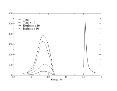
Figure 9: Photocurrent as function of photoelectron energy in Ry. The zero level corresponds to the bottom of the valence band. The spectrum is excited 7.5 Ry above threshold, and the photoelectron mean free path is approximated by a constant corresponding to $\Gamma_{p}=0.3$ Ry.

In Fig. (9) we show results for plasmon losses with an excitation energy 7.5 Ry above threshold. These and the following results correspond to aluminium, and the lattice ${\mathbf{G}}$ vector, which acts as momentum source, has a parallel component of 0.7 a.u. and a component of 2.6 a.u. perpendicular to the surface. The extrinsic losses dominate, and the total loss is somewhat smaller than the sum of the extrinsic and intrinsic ones. However, we have observed that interference depend on the direction of the photocurrent even at 7.5 Ry. The two loss mechanisms are therefore not completely decoupled even at 1̃00 eV. In Fig. (10) we have lowered the excitation energy to 4.5 Ry. In this case the interference is much stronger, and the extrinsic and intrinsic parts interfere destructively.

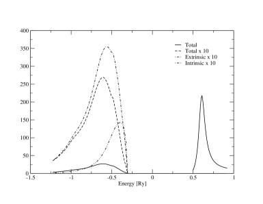
Figure 10: Photocurrent excited 4.5 Ry above threshold. $\Gamma_{p}=0.3$ Ry. Notations as in Fig. 9

Finally one may ask how the quasi particle line shape is modified by the transport and interference effects. In our calculations we have obtained almost negligible effects. As an example, I show the quasi particle region at an excitation energy of 2.5 Ry (Fig. (11)). The broadening that is seen without any particle-hole effects comes from the finite mean free path which smears the momentum selection rules normal to the surface.

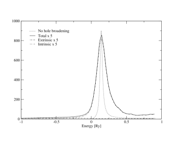
Figure 11: Broadening of the quasi particle peak at normal emission. $\omega_{i}=2.5$ Ry. For notations see Fig. 9

As remarked above, the first-order $GW$ theory gives a rather crude representation of the shape of the plasmon satellites. The description will be improved by going to second order in transition amplitudes as described in Sec. 4.2. This higher-order approximation is still simple enough to allow for numerical evaluations. Within the approximations used above for the first-order results the second-order amplitudes can again be obtained by propagating one-electron orbitals which makes the calculation manageable. As the excitation energy is further increased, more and more plasmon satellites will result in experimental spectra. At sufficiently high energies, the energy losses can be described by semi-classical approaches in which the photoelectron is considered as a classical particle which moves along a certain trajectory[43, 39] or by an integral equation which approximates the losses at high energies[8]. We expect that explicit quantum-mechanical calculations up to second order in $W$ will cover the energy window up to the limit where these simpler methods are applicable. Extensions to second order along the lines given here are on the way and will be presented elsewhere.

5 Concluding remarks

In this paper I have discussed how techniques from non-equilibrium Green’s function theory may be used to develop useful approximations as well as for establishing general results such as the structure of the no-loss quasi particle part of the spectrum. Although I have discussed energy losses in some detail in the second part, I would like to emphasis that it is the no-loss quasi particle part that is usually of primary interest in experimental studies. The current computational schemes in which the photoelectron moves in a non-Hermitian optical potential is essentially correct. The necessary ingredients are here sufficiently accurate approximations for the self-energy including its imaginary part. It may be necessary to account for its non-locality at least in some approximate way. The proper evaluation of matrix elements the screened optical field is another area where improvements may be necessary. Especially in spectral regions where the photoelectron self-energy is rapidly varying it may also be necessary to account for the vertex corrections discussed in Sec. 3.

In order to treat energy losses below the main quasi-particle peak, a regrouping of diagrams in many-body perturbation theory has been proposed. In each order the partial sums have a Golden-Rule-like form which guarantees positive spectral intensities. This way of regrouping may be useful also in other problems involving spectral intensities. One such problem is how to improve the one-electron spectral function beyond $GW$ theory.

Some new model results for valence-electron photoemission have been presented, and more realistic results are on the way. The model results confirm the expectations that interference effects modify the shape and strength of plasmon satellites also quite far away from the excitation threshold, whereas the quasi-particle part is little modified. Based on our ongoing work we intend to compare fully quantum-mechanical results to semi-classical descriptions of the photoelectron transport away from threshold.

References

References

- [1] A. Einstein. Ann. Physik, 17:132, 1905.
- [2] C. N. Berglund and W. E. Spicer. Phys. Rev., 136:A1030, 1964.
- [3] W. L. Schaich and N. W. Ashcroft. Phys. Rev. B, 3:2452, 1970.
- [4] G. D. Mahan. Phys. Rev. B, 2:4334, 1970.
- [5] C. Caroli, D. Lederer-Rozenblatt, B. Roulet, and D. Saint-James. Phys. Rev. B, 8:4552, 1973.
- [6] D. C. Langreth. Phys. Rev. B, 3:3120, 1971.
- [7] J. J. Chang and D. C. Langreth. Phys. Rev. B, 5:3512, 1972.
- [8] J. J. Chang and D. C. Langreth. Phys. Rev. B, 8:4638, 1973.
- [9] D. C. Langreth. In B. I Lundqvist and S. Lundqvist, editors, Collecive Properties of Physical Systems. Academic, New York, 1973.
- [10] P. J. Feibelman and D. E. Eastman. Phys. Rev. B, 10:4932, 1974.
- [11] J.B. Pendry. Surf. Sc, 57:1976, 1974.
- [12] A. Liebsch. Phys. Rev. B, 13:544, 1976.
- [13] A. Liebsch. In J. Treusch, editor, Festkörperprobleme, volume 19, page 209. Vieweg, Braunschweig, 1979.
- [14] C.-O. Almbladh. Physica Scripta, 32:341, 1985.
- [15] W. Bardyszewski and L. Hedin. Physica Scripta, 32:439, 1985.
- [16] W. Schattke and M. A. Van Hove:, editors. Solid-State Photoemission and Related Methods. Wiley-VCH, Weinheim, 2003.
- [17] S. Hüfner. Photoelectron spectroscopy, volume 82. Springer, Berlin, 1995.
- [18] S. D. Kevan (Ed.). Angle-resolved photoemission. Elsevier, Amsterdam, 1992.
- [19] I. Adawi. Phys. Rev., 134:A788, 1964.
- [20] H. Hermeking and R. P. Wehrum. J. Phys. C, 8:3468, 1973.
- [21] M. Gell-Mann and M. L. Goldberger. Phys. Rev., 91:398, 1953.
- [22] L. V. Keldysh. J. Exp. Theor. Phys. (USSR), 47:1515, 1964. [Transl. Soviet Phys. JETP 20, 1018 (1965)].
- [23] L. P. Kadanoff and G. Baym. Phys. Rev., 124:287, 1961.
- [24] L. P. Kadanoff and G. Baym. Quantum Statistical Mechanics. Benjamin, New York, 1962.
- [25] G. Baym. Phys. Rev., 127:1391, 1962.
- [26] L. Hedin. Phys. Rev, 139:A796, 1965.
- [27] J. Inglesfield. J. Phys. C, 16:403, 1983.
- [28] A. Liebsch. Electronic excitations at metal surfaces. Plenum, New York, 1997.
- [29] W. Schattke. Progr. Surf. Sci, 54:211, 1997.
- [30] E. E. Krasovskii and W. Schattke. Phys. Rev. B, 63:235112, 2001.
- [31] L. Hedin, J. Michiels, and J. Inglesfield. Phys. Rev. B, 58:15565, 1998.
- [32] J. D. Lee, O. Gunnarsson, and L. Hedin. Phys. Rev. B, 60:8034, 1999.
- [33] T. McMullen, B. Bergersen, and P. Jena. J. Phys. C, 9:975, 1976.
- [34] C.-O. Almbladh. Phys. Rev, 34:3798, 1986.
- [35] G. D. Mahan. Phys. Stat. Sol. B, 55:703, 1973.
- [36] J. W. Gadzuk and M. J. Sunjic. Phys. Rev. B, 12:524, 1975.
- [37] D. Chastenet and P. Longe. Phys. Rev. Lett., 91:44, 1980.
- [38] A. C. Simonsen, F. Yoberoo, and S. Tougard. Phys. Rev. B, 56:1612, 1997.
- [39] L. Hedin. General theory for core-electron photoemission. In W. Schattke and M. A. Van Hove (Eds.), editors, Solid-State Photoemission and Related Methods. Wiley-VCH, Weinheim, 2003.
- [40] D. C. Langreth. In J. T. Devreese and E. van Doren, editors, Linear and Nonlinear Electron Transport in Solids, pages 3 – 32. Plenum, New York, 1976.
- [41] B. Holm and U. von Barth. Phys. Rev. B, 57:2108, 1998.
- [42] F. Bechstedt, R. Enderlein, and D. Reichart. Phys. Stat. Sol. B, 117:261, 1983.
- [43] C.-O Almbladh and L. Hedin. Beyond the one-electron model: Many-electron effects in atoms, molecules, and solids. In E. E. Koch, editor, Handbook on Synchrotron Radiation, volume 1b, page 607. North-Holland, Amsterdam, 1983.