Semilinear response

Abstract

We discuss the response of a quantum system to a time-dependent perturbation with spectrum $\Phi(\omega)$. This is characterised by a rate constant $D$ describing the diffusion of occupation probability between levels. We calculate the transition rates by first order perturbation theory, so that multiplying $\Phi(\omega)$ by a constant $\lambda$ changes the diffusion constant to $\lambda D$. However, we discuss circumstances where this linearity does not extend to the function space of intensities, so that if intensities $\Phi_{i}(\omega)$ yield diffusion constants $D_{i}$, then the intensity $\sum_{i}\Phi_{i}(\omega)$ does not result in a diffusion constant $\sum_{i}D_{i}$. This ‘semilinear’ response can occur in the absorption of radiation by small metal particles.

Quantum mechanics Fluctuation phenomena, random processes, noise, Brownian motion. Transport processes.Electronic transport in mesoscopic systems.Optical properties of low dimensional structures.

1. Introduction. We describe a previously unremarked phenomenon concerning the response of a quantum system to a time-dependent perturbation. The effect is significant if the characteristic frequency scale of the perturbation $\omega_{0}$ obeys $\varrho\hbar\omega_{0}<1$, where $\varrho$ is the density of states. Our analysis is an extension of linear-response theory, in that it too relies on first-order perturbation theory, in our case to derive rate constants for transitions between levels. The rate constants are used in a master equation, which is then analysed non-perturbatively. The response obtained is always linear in the intensity of the driving perturbation, but in some circumstances the response is not a linear functional of its spectrum. This point will stated more precisely below. Conventional linear response always describes the initial response of a system, whereas our theory also considers how the response may differ after an initial transient. The data plotted in figure 1 (which is explained later) show that the predictions can differ by orders of magnitude.

We characterise the response of the system by the rate $\dot{E}\equiv{\rm d}E/{\rm d}t$ at which its energy is increased by the action of the perturbation. This is directly related to experimentally observable quantities, such as the absorption of radiation by small metallic particles in an electromagnetic field. The expectation from conventional linear-response theory (see for example [2]) is that the rate of absorption is a linear functional of the spectral intensity $\Phi(\omega)$ of the radiation:

$$\dot{E}=\int_{0}^{\infty}{\rm d}\omega\ \alpha(\omega)\,\Phi(\omega)$$ (1)

where $\alpha(\omega)$ is a frequency-dependent absorption coefficient. This expression satisfies two requirements for linearity: if an intensity function $\Phi_{i}(\omega)$ results in a response $\dot{E}_{i}$, then (1) implies that for some constant $\lambda$

$$\Phi(\omega)\mapsto\lambda\Phi(\omega)\ \ \ \ \ \ \ \Longrightarrow\ \ \ \dot{E}\mapsto\lambda\dot{E}$$ (2)

$$\Phi(\omega)\mapsto\sum_{i}\Phi_{i}(\omega) \ \ \ \Longrightarrow\ \ \ \dot{E}\mapsto\sum_{i}\dot{E}_{i}\ .$$ (3)

In this letter we introduce a new form of linear-response theory, which satisfies (2) but not (3), and which we therefore term semilinear response theory. In the limiting case $\varrho\hbar\omega_{0}\ll 1$ we show that the absorption rate is approximated by

$$\dot{E}=\biggl{[}\int_{0}^{\infty}{\rm d}\omega\ \mu(\omega)\,\Phi^{-1}(\omega)\biggr{]}^{-1}$$ (4)

where $\mu(\omega)$ will be specified later. Equation (4) clearly satisfies condition (2), but not (3). This is a consequence of the fact that (4) is a weighted harmonic average of the spectral intensity function, $\Phi(\omega)$. Reference [3] discusses a model for a quantum dot coupled to a conducting ring, where the DC conductance is also obtained by a harmonic averaging procedure. In that case, however, harmonic averaging is relevant because of the specific structure of the Hamiltonian of that system. By contrast, the results described here relating the AC response to $\Phi(\omega)$ are applicable to generic systems.

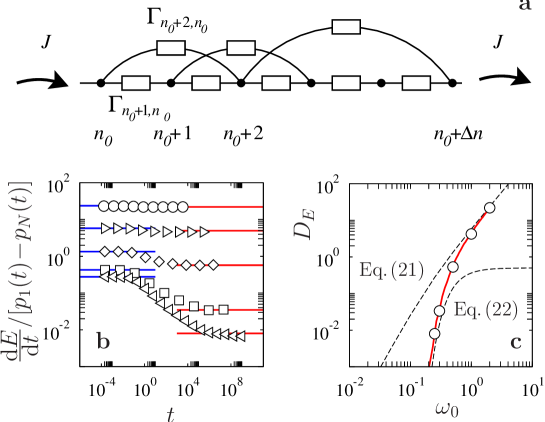
Figure 1: (a) The network of transitions between states is analogous to a random resistor network. (b) Rate of energy absorption divided by difference in the occupation probabilities of the lowest and the highest states, showing crossover from an initial transient to a steady state. The numerical simulations of (11) employ random-matrix eigenvalues with $\beta=1,\,\sigma^{2}=1,\,\varrho=1$, $N_{\rm p}=3$, and $\Phi(\omega)=\varepsilon^{2}\,\exp(-|\omega|/\omega_{0})/\omega_{0}$, for $\varepsilon^{2}=1$ and $\omega_{0}=2$ ($\circ$), $1$ ($\triangleright$), $0.5$ ($\Diamond$), $0.3$ ($\Box$), and $0.25$ ($\triangleleft$). The results were averaged over $200$ realisations of $\hat{\cal H}_{j}$. The asymptotes are: left, linear-response for the initial transient [eq.(21)], right, steady state determined by network model [eq.(14)]. (c) Energy-diffusion constant $D_{E}$ vs. $\omega_{0}$. Symbols are long-time asymptotes from figure 1b. The solid line is the semilinear response obtained by solving (14), averaging over $20$ realisations. Also shown are linear-response approximation [eq.(21)], asymptote to semilinear-response theory [eq.(22)].

Our approach is based upon an observation about the response of quantum systems to low-frequency perturbations. We discuss a system which absorbs a finite amount of energy, $E_{0}$, and consider taking the limit as the characteristic frequency $\omega_{0}$ of the perturbation approaches zero. The number of quanta that the system absorbs, $E_{0}/\hbar\omega_{0}$, diverges as $\omega_{0}\to 0$. In order to understand the response of a quantum system to low-frequency perturbations, we must therefore consider multiple excitations. We describe the excitation of the system by a master equation, describing the probability $p_{n}(t)$ that the system is in state with level number $n$ at time $t$. If this master equation is treated in perturbation theory, we recover conventional linear-response theory. However, our non-perturbative treatment yields distinctive differences from the usual linear-response results.

Our results are quite generally applicable, but it may be helpful to bear in mind a specific example, namely a single electron trapped inside an irregularly shaped enclosure, subjected to fluctuating electric fields. This is a simplified model for the absorption of electromagnetic radiation by small metallic particles. In a classic paper, Gorkov and Eliashberg [4] predicted a quantum size effect, where the absorption of radiation would show distinctive structures for frequencies close to the frequency $(\varrho\hbar)^{-1}$ (here $\varrho$ is the density of states of single electron excitations at the Fermi energy). The energy levels were assumed to have the same statistical properties as random matrices, and the absorption was calculated using random matrix models introduced by Dyson [5], discussed in [6]. We start from the same model and arrive at very different conclusions. We remark that despite intensive investigation, there is no clear experimental evidence for the validity of the theory proposed in [4].

2. The Hamiltonian. We denote the Hamiltonian in the absence of external fields by $\hat{\mathcal{H}}_{0}$. The perturbation is described by a set of $N_{\rm p}$ operators $\hat{\mathcal{H}}_{j}$ multiplied by time-dependent fields $X_{j}(t)$:

$$\hat{\mathcal{H}}(t)=\hat{\mathcal{H}}_{0}+\sum_{j=1}^{N_{\rm p}}X_{j}(t)\hat{\mathcal{H}}_{j}\ .$$ (5)

In the case where the theory is applied to very small metal particles in an electromagnetic field, $\hat{\mathcal{H}}_{0}$ is the Hamiltonian for quasiparticle excitations, and the $\hat{\mathcal{H}}_{j}$ are operators representing coupling of quasiparticles to the $N_{\rm p}=3$ components of the electric field, $X_{j}(t)$. The operators $\hat{\mathcal{H}}_{j}$ are not simple dipole operators, because they must take account of screening of the externally applied perturbation by polarisation charges [7, 8].

The fields are not monochromatic, and their components $X_{j}(t)$ are random functions of time, satisfying

$$\langle X_{j}(t)\rangle{=}0\quad\mbox{and}\quad\langle X_{i}(t)X_{j}(t^{\prime})\rangle{=}\delta_{ij}\phi(t{-}t^{\prime})\,\,$$ (6)

(angular brackets denote averages). The fields have a spectral intensity $\Phi(\omega)$, defined by

$$\Phi(\omega)=\int_{-\infty}^{\infty}{\rm d}\tau\ \phi(\tau)\exp({\rm i}\omega\tau)\,.$$ (7)

In the numerical examples below, we take $\Phi(\omega)=\varepsilon^{2}\exp(-|\omega|/\omega_{0})/\omega_{0}$ where $\omega_{0}$, $\varepsilon$ are constants. An exponential dependence with $\omega_{0}=k_{\rm B}T/\hbar$ is a natural choice if the system is excited thermally.

3. Master equation. First consider the rate for transitions between eigenstates of $\hat{\cal H}_{0}$. Expand the solution $|\psi(t)\rangle$ of the Schrödinger equation ${\rm i}\hbar{\rm d}|\psi\rangle/{\rm d}t=\hat{\mathcal{H}}(t)|\psi\rangle$

$$|\psi(t)\rangle=\sum_{n}a_{n}(t)\exp(-{\rm i}E_{n}t/\hbar)\ |\varphi_{n}\rangle$$ (8)

where $\hat{\mathcal{H}}_{0}|\varphi_{n}\rangle=E_{n}|\varphi_{n}\rangle$ and the energies are ordered according to the index $n$. The amplitudes $a_{n}(t)$ satisfy:

$$\dot{a}_{n}={-{\rm i}\over{\hbar}}\sum_{m}\exp({\rm i}\omega_{nm}t)\sum_{j=1}^{N_{\rm p}}\mathcal{H}_{nm}^{(j)}X_{j}(t)a_{m}$$ (9)

where $\mathcal{H}_{nm}^{(j)}=\langle\varphi_{n}|\hat{\mathcal{H}}_{j}|\varphi_{m}\rangle$ and $\omega_{nm}=(E_{n}-E_{m})/\hbar$. Solving perturbatively for the initial condition $a_{n}(0)=\delta_{nm}$ one obtains an expression for $a_{n}(t)$ and hence for the probability $p_{n}(t)=\langle|a_{n}(t)|^{2}\rangle$ to be in the $n^{\rm th}$ state. For $n\neq m$ we have $p_{n}(t)=\Gamma_{nm}t+O(t^{2})$, where the rate constants are given by a version of Fermi’s golden rule

$$\Gamma_{nm}\ \ =\ \ \frac{1}{\hbar^{2}}\ \Phi(\omega_{nm})\ \sum_{j=1}^{N_{\rm p}}|\mathcal{H}_{nm}^{(j)}|^{2}\,.$$ (10)

The expression for $p_{n}$ is valid for times sufficiently short that $1-p_{m}\ll 1$, but large enough that $\omega_{0}t\gg 1$. These conditions are compatible for a sufficiently small $\varepsilon$.

The rate constants can be used to write the master equation for the occupation probabilities $p_{n}(t)$:

$${{\rm d}p_{n}\over{{\rm d}t}}=\sum_{m}\Gamma_{nm}(p_{m}-p_{n})\,.$$ (11)

This master-equation ignores interference effects, which average away on long timescales.

Our model (5), (6) describes excitation of a quantum system due to a perturbation. In practical applications, the system may also be subject to relaxation effects. The master-equation model can then be augmented with terms representing relaxation processes. These additional terms could represent the transfer of energy from electronic excitations into phonons or photons. Electron-electron interactions could also be included, although these represent re-arrangement of energy within the electronic system rather than relaxation. The lifetime for an electron to emit photons or phonons diverges as the energy of excitation of the electron approaches zero. For systems excited by low-frequency fields, electrons may therefore be excited by many quanta before their relaxation rate is significant. Thus our approach is in contrast with conventional linear response theory [11] which implicitly assumes that multiple excitations are not relevant.

In the case of absorption of electromagnetic radiation by small conducting particles, reference [4] shows that phonons do not cause relaxation at low frequencies, so that emission of photons is the dominant relaxation mechanism. In this case it is easy to see that there is multiple excitation when the intensity of radiation at frequency $\omega_{0}$ is large compared to the intensity of black-body radiation at temperature $T=\hbar\omega_{0}/k_{\rm B}$. This condition is easily satisfied at the microwave or far-infrared frequencies which are relevant to experimental studies on the effect discussed in [4].

4. Energy diffusion and resistor networks. We are interested in the long-time behaviour of the master equation (11). The coarse-grained occupation probabilities obey a continuity equation:

$$\partial_{t}p(n,t)+\partial_{n}J(n,t)=0$$ (12)

with probability flux $J$. We argue below that the coarse-grained occupation probability obeys Fick’s law, ${J=-D\partial p/\partial n}$, so that $p(n,t)$ obeys a diffusion equation

$$\partial_{t}p=\partial_{n}\left[D\partial_{n}p\right]\,.$$ (13)

In order to determine $D$ we make use of the analogy between (11) and Kirchoff’s equation for a resistor network (illustrated in figure 1a): nodes $n$ and $m$ are connected by conductances $G_{nm}$. If a current $I_{n}$ is supplied at node $n$, the potentials $V_{n}$ satisfy

$$I_{n}=\sum_{m}G_{nm}(V_{n}-V_{m})\,.$$ (14)

The probabilities $p_{n}$ in (11) correspond to the potentials $V_{n}$, the rates $\Gamma_{nm}$ to the conductances $G_{nm}$, and in the steady state $I_{n}\equiv-{\rm d}p_{n}/{\rm d}t=0$ at all the nodes. Coarse graining is achieved by considering a truncated network segment of length $\Delta n\gg 1$ as illustrated in figure 1a, with a current $J$ is injected into one end and extracted at the other end. This finite segment is described by an equation in the form of (14) with ${I_{n}=J\delta_{n,n_{0}}-J\delta_{n,n_{0}+\Delta n}}$, resulting in a potential difference $\Delta V=V_{n_{0}+\Delta n}-V_{n_{0}}$. We expect that $\Delta V/\Delta n$ approaches a limit as $\Delta n$ increases, implying a ‘coarse grained’ Fick’s law: ${J\approx-D(p_{n_{0}{+}\Delta n}-p_{n_{0}})/\Delta n}$, which is analogous to Ohm’s Law. Thus $D/\Delta n$ is the conductance of the segment, and $D$ is obtained as $D=-J\lim_{\Delta n\to\infty}{\Delta n/\Delta V}$. We remark that Miller and Abrahams [9] introduced random resistor models in studies of spatial (as opposed to energy) diffusion in disordered systems.

In what follows we discuss expressions for $D$ in two limiting cases. When the rate constants are negligible for all but nearest-neighbour transitions, the resistance $(D/\Delta n)^{-1}$ is the sum of resistors in series, leading to

$$D=\bigg{(}\lim_{\Delta n\to\infty}\frac{1}{\Delta n}\sum_{n=n_{0}}^{n_{0}{+}\Delta n}\Gamma_{n,n+1}^{-1}\bigg{)}^{-1}\equiv\left\langle\Gamma_{n,n+1}^{-1}\right\rangle^{-1}$$ (15)

To show that Fick’s law holds in the limit considered here, it suffices to show that (15) yields a finite result for $D$ (an example is given in equation (22) below). It is an immediate consequence of the nature of the harmonic average that the diffusion constant is significantly reduced by the presence of ‘bottlenecks’, that is links with very low transition rates [10]. Reference [3] considers the consequences of this for energy diffusion in a model for the DC response of a quantum dot coupled to a conducting ring.

We turn to the other extreme case, where many transitions have significant weight (not just to near neighbours). We may assume that the potential changes linearly along the network ($p_{n}\propto n$) and find that

$$D=\big{\langle}\ {\textstyle{1\over 2}}\sum_{m}(m-n)^{2}\Gamma_{n,m}\big{\rangle}\,.$$ (16)

where the angular brackets means averaging over $n$ as in equation (15). To derive this, note that the contribution of bond of length $\Delta n=(m-n)$ to the current is proportional to the potential drop and hence to $\Delta n$. Furthermore the number of bonds of length $\Delta n$ passing through a given section gives a further factor $\Delta n/2$.

5. Rate of absorption of energy. The expectation value of the energy of the system is

$$E(t)=\sum_{n}p_{n}(t)E_{n}\,.$$ (17)

When many states are excited, the sum may be approximated by an integral. Applying (13), the rate at which energy is absorbed is

$$\dot{E}\!=\!\int\!\!{\rm d}n\,E_{n}\partial_{n}[D\partial_{n}p]=\!-\!\int\!\!{\rm d}E\,\varrho D_{E}{\partial p\over{\partial E}}\,.$$ (18)

This equation shows that the rate of energy absorption $\dot{E}$ is proportional to the energy-diffusion coefficient ${D_{E}=D/\varrho^{2}}$, a principle that was introduced in [12].

6. An example of semilinear response. Consider the case where $\varrho\hbar\omega_{0}\ll 1$. Here the rate constants (10) decrease very rapidly as the separation in energy increases, and we can neglect all of the rate constants $\Gamma_{nm}$ other than those describing nearest neighbour coupling. The diffusion constant ${D_{E}=D/\varrho^{2}}$ is then estimated via equation (15). It is clear that large gaps in the spectrum create ‘bottlenecks’ which slow the diffusion of probability. We define $P(S){\rm d}S$ as the probability that the normalised spacing between two successive levels $(E_{n+1}-E_{n})\varrho$ is in the interval $[S,S+{\rm d}S]$. We assume that the matrix elements $\mathcal{H}_{nm}^{(j)}$ are independent Gaussian random variables with variance $\sigma^{2}$ and zero mean, independent of the energy levels. We write $\mathcal{H}_{nm}^{(j)}=\sigma x_{nm}^{(j)}$ with Gaussian random variables $x_{nm}^{(j)}$, each with zero mean and unit variance, then substitute (10) into (15) and find

$$D_{E}\!=\!{\sigma^{2}\over{(\varrho\hbar)^{3}}}\biggl{[}\int\!\!\frac{{\rm d}{\bf x}\,{\rm e}^{-{\bf x}^{2}/2}}{(2\pi)^{N_{\rm p}/2}{\bf x}^{2}}\biggr{]}^{-1}\biggl{[}\int_{0}^{\infty}\!\!\!\!\!\!{\rm d}\omega\frac{P(\varrho\hbar\omega)}{\Phi(\omega)}\biggr{]}^{-1}\,.$$ (19)

Eq. (19) is an example of semilinear response, in the form of eq.(4). Assuming that $\Phi(\omega)$ decreases rapidly when $\omega\gg\omega_{0}$, the integral in (19) is dominated by the tail of the level spacing distribution. Denoting the second term (with the integral over ${\rm d}{\bf x}$) by $W$, we find that $W=1$ for $N_{\rm p}=3$. For $N_{\rm p}=1,2$ we find $W=0$, so that $D_{E}=0$, implying that the spread of probability is sub-diffusive.

7. Linear-response theory. Now we contrast (19) with conventional linear-response theory. We assume that the initial probability $p_{n}(0)$ is a smooth function of the energy of the state. We differentiate (11), substitute in (17), and expand $p_{m}-p_{n}$ to first order in $E_{n}-E_{m}$. Interchanging the indices $n$ and $m$ and averaging the two expressions for the double sum gives:

$$\dot{E}=-{\textstyle{\frac{1}{2}}}\sum_{n,m}(E_{m}-E_{n})^{2}\Gamma_{nm}\frac{\partial p}{\partial E}\,.$$ (20)

We can identify $D_{E}$ by comparison with (18). After substitution of (10) we obtain an expression in terms of the two-level correlation function $R_{2}(\epsilon)=\sum_{nm}\langle\delta(E-E_{n})\delta(E+\epsilon-E_{m})\rangle/\varrho^{2}$ (we use the notation of [6])

$$D_{E}=N_{\rm p}\sigma^{2}\hbar\varrho\int_{0}^{\infty}\!\!\!{\rm d}\omega\,\omega^{2}\,R_{2}(\hbar\omega)\Phi(\omega)\,.$$ (21)

This a linear functional of the spectral intensity $\Phi(\omega)$, leading to and expression of the form (1). Equation (21) is a version of the ‘Kubo formula’ of linear-response theory and is equivalent to a result obtained by Gorkov and Eliashberg [4]. It is subject to the criticism that it only describes the initial response of the system (figure 1b): after a short transient, the probabilities may cease to be given accurately by a smooth function of the energy, leading to a very different rate of absorption, such as that given by (19). Conventional linear-response theory [11] implicitly assumes that strong relaxation prevents level-number diffusion from exploring the ‘bottlenecks’.

Finally we remark that if the initial probability $p_{n}(0)$ is a smooth of level number $n$ instead of $E_{n}$, a slightly modified form of linear-response theory is obtained [11].

8. Random-matrix models and numerical experiments. We now compare the calculation of $D_{E}$ using (19) with conventional linear-response theory (21), assuming random matrix models for $P(S)$ and $R_{2}(\epsilon)$. Although the spectra of complex quantum systems differ, their statistical properties are very similar and can be calculated for suitably defined random-matrix ensembles [6]. There are three ‘universal’ ensembles, labelled by an integer index $\beta\in\{1,2,4\}$. For $P(S)$ we use the ‘Wigner surmise’, $P(S)\sim a_{\beta}S^{\beta}\exp(-c_{\beta}S^{2})$, with $a_{\beta}$ and $c_{\beta}$ chosen so that $P(S)$ is normalised with mean value unity. The diffusion coefficient (19) depends on the large separations, so that we require accurate information about the values of $P(S)$ for large argument: precise information about the large $S$ asymptotics is given in [6], but for the moderately large values of $S$ that are probed by our numerical studies, the Wigner surmise gives more accurate results. We also require $R_{2}(\epsilon)$, to evaluate (21). Here it is the behaviour for small spacings that is of most interest, where $R_{2}(\epsilon)=k_{\beta}(\varrho\epsilon)^{\beta}+O(\epsilon^{\beta+1})$ with universal constants $k_{\beta}$.

We illustrate the theory by comparing the predictions of (19) and (21) for a spectral intensity $\Phi(\omega)=\varepsilon^{2}\exp(-|\omega|/\omega_{0})/\omega_{0}$ and $\beta=1$, using the Wigner surmise for $P(S)$. As $\omega_{0}\to 0$, equation (19) predicts that $D_{E}$ approaches zero in a non-analytic fashion:

$$D_{E}=(\varepsilon^{2}\sigma^{2}/{2\varrho\hbar})\,\exp\{-1/[\pi(\varrho\hbar\omega_{0})^{2}]\}\,.$$ (22)

This is dramatically different from the result of conventional linear response theory (21) where, for small values of $\omega_{0}$, we find $D_{E}\sim C_{\beta}N_{\rm p}\sigma^{2}\varepsilon^{2}(\hbar\varrho)^{\beta+1}\omega_{0}^{\beta+2}$ (for some universal constants $C_{\beta}$).

Figure 1b,c shows numerical results for simulations using random-matrix energy levels, with $\beta=1$, $\varepsilon=1$, $\sigma^{2}=1$, $N_{\rm p}=3$, and $\varrho=1$. The data in figure 1b are obtained by a simulation of (11) with (17). We use GOE [5] random matrices of dimension $N=4000$ and an exponential initial distribution $p_{n}\propto\exp(-E_{n}/\Delta E)$ with $\varrho\Delta E=100$. After an initial transient both $\dot{E}$ and $(p_{1}(t)-p_{N}(t))$ decrease, their ratio approaching a limit which (using (18)) we identify as $\varrho D_{E}$. These limiting values of $D_{E}$ are plotted as symbols in figure 1c. The data for the resistor network (solid line) was obtained by solving Kirchoff’s law for a network with $N=4000$ nodes, using singular-value decomposition.

9. Summary. We have considered the non-perturbative solution of a master equation describing transitions between levels. Its solutions are in general diffusive for large times, with a diffusion constant obtained from the conductivity of a random resistor network. When the characteristic frequency $\omega_{0}$ is small ($\varrho\hbar\omega_{0}\ll 1$), only transitions between neighbouring levels are significant, analogous to resistors in series. The diffusion constant is then the harmonic mean of the rate constants. It is determined by the tail of the level spacing distribution and is an example of semilinear response.

10. Acknowledgements. We thank Y. Gefen for helpful discussions. This research was supported by the Vetenskapsrådet and by the Israel Science Foundation (grant No.11/02).

References

- [1]
- [2] M. Toda, R. Kubo and N. Saito , Statistical Physics II, Springer Berlin (1992).
- [3] D. Cohen, T. Kottos and H. Schanz, cond-mat/0505295 (2005), J. Phys. A 39, 11755 (2006).
- [4] L. P. Gorkov and G. M. Eliashberg, Zh. Eksp. Teor. Fiz., 48, 1407, (1965) (English transl. JETP, 21, 940, (1965)).
- [5] F. J. Dyson, J. Math. Phys., 3, 157, (1962).
- [6] M. L. Mehta, Random Matrices, Academic, New York, (1991).
- [7] S. Strässler, T. M. Rice and P. Wyder, Phys. Rev., B6, 2575, (1972).
- [8] E. J. Austin and M. Wilkinson, J. Phys. Condens. Matter, 5, 8461, (1993); M. Wilkinson and B. Mehlig, ibid. 12, 10481, (2000).
- [9] A. Miller and E. Abrahams, Phys. Rev., 120, 745, (1960).
- [10] S. Alexander, J. Bernasconi, W. R. Schneider, R. Orbach, Rev. Mod. Phys., 53, 175-98, (1981).
- [11] A. Kamenev and Y. Gefen, Int. J. Mod. Phys. B, 9, 751 (1995).
- [12] M. Wilkinson, J. Phys. A, 21, 4021, (1988).