Towards Universal Topological Quantum Computation in the $\nu=5/2$ Fractional Quantum Hall State

Abstract

The Pfaffian state, which may describe the quantized Hall plateau observed at Landau level filling fraction $\nu~{}=~{}5/2$, can support topologically-protected qubits with extremely low error rates. Braiding operations also allow perfect implementation of certain unitary transformations of these qubits. However, in the case of the Pfaffian state, this set of unitary operations is not quite sufficient for universal quantum computation (i.e. is not dense in the unitary group). If some topologically unprotected operations are also used, then the Pfaffian state supports universal quantum computation, albeit with some operations which require error correction. On the other hand, if certain topology-changing operations can be implemented, then fully topologically-protected universal quantum computation is possible. In order to accomplish this, it is necessary to measure the interference between quasiparticle trajectories which encircle other moving trajectories in a time-dependent Hall droplet geometry.foot

I Introduction

The fractional quantum Hall regime DasSarma97 contains a cornucopia of Abelian fractional quantum Hall states, i.e. states whose quasiparticle excitations have Abelian braiding statistics stat ; Abelian-expt . It is possible that an even more wonderful phenomenon may occur there: non-Abelian quantum Hall states. The strongest candidate is the $\nu=5/2$ quantum Hall state. This state is quite robust in the highest-mobility samples Xia04 , and numerical studies indicate that the Pfaffian state Moore91 ; Greiter92 , which has excitations exhibiting non-Abelian braiding statistics Nayak96c ; Gurarie97 ; Tserkovnyak03 ; Read96 ; Read00 ; Ivanov01 ; Stern04 ; Fradkin98 ; Fradkin99 , has large overlap with the exact ground state for small numbers of electrons at this filling fraction Morf98 ; Rezayi00 . An experiment has been proposed DasSarma05 which would determine if the $\nu=5/2$ state is, indeed, in the universality class of the Pfaffian state by observing the signature of non-Abelian statistics: a degenerate set of multi-quasiparticle states which cannot be distinguished locally but can be distinguished by a non-Abelian analogue of the Aharonov-Bohm interference measurement. In the two quasiparticle case, this is simply the observation of a topologically-protected qubit Kitaev97 ; Freedman01a . In the presence of many pairs of quasiparticles, all kept far apart, the topologically-degenerate ground states form many qubits. These states are locally indistinguishable. If the environment interacts only locally with the system, it cannot act on these qubits. Braiding the quasiparticles around each other, an intrinsically non-local operation, transforms the qubits. These gates are exact because small deformations of the qusiparticle trajectories do not affect their braiding topology. However, there is a sense in which the Pfaffian state is not quite non-Abelian enough: the set of all possible braiding operations only gives a finite set of unitary transformations on the qubits. Thus, with these operations, it is not possible to perform any desired unitary transformation, which would be necessary for a universal quantum computer.

In this paper, we suggest ways in which this apparent shortcoming of the Pfaffian state (and, by implication, the $\nu=5/2$ quantum Hall state) can be circumvented. The first, more pedestrian, approach is to use some non-topological operations. Consider, for instance, what happens when two quasiparticles are brought close together. The degeneracy between the two states of their qubit is broken. Since unitary evolution in time will now cause a phase difference to develop between the two states of the qubit, we thereby implement a phase gate. We explain how a universal quantum computer can be constructed using these ideas. The second, more interesting, approach relies on (1) the construction by Bravyi and Kitaev BK of a universal set of gates for the Pfaffian state which exploits topology change in an abstract context in which there are no restrictions on the global topology of spacetime (using, for instance, overcrossings and undercrossings, which seem unlikely to be realized in a system of electrons confined to a plane ); and (2) the observation that their operations actually can be implemented in a way that remains entirely in the plane so long as one is able to measure the interference between trajectories encircling quasiparticles which are moving, merging, and splitting – i.e. interference in a time-dependent background Hall fluid. We note, in passing, that $\nu=12/5$ may also be a non-Abelian state, specifically one of the states proposed by Read and Rezayi Read99 . It may be particularly interesting – even though it is seen more weakly – because, if it is indeed a Read-Rezayi state Read99 , braiding operations alone are sufficient to implement any unitary transformation within desired accuracy – i.e. it supports topologically-protected universal quantum computation Freedman02 . In the event that the $\nu=12/5$ state proves to be simply an Abelian state or to have too small an energy gap to permit manipulation, the protocols described in this paper, if they can be experimentally realized, would save the day by boosting the computational power of the $\nu=5/2$ state so that it, too, can be regarded as a universal quantum computer. Furthermore, the basic architecture which we describe in sections II and III is relevant to the $\nu=12/5$ state as well.

II Qubits in the Pfaffian State

In this paper, we will assume that the $\nu=5/2$ plateau is in the universality class of the Pfaffian quantum Hall state. In this section, we list some basic facts about the Pfaffian quantum Hall state and introduce some notation which will be useful in the following sections. The goal is to describe the qubits which arise when many quasiparticles are present.

The Pfaffian wavefunction Moore91 ; Greiter92 takes the form:

$$\Psi_{\rm g.s.}(z_{j})~{}=~{}\prod_{j<k}(z_{j}-z_{k})^{2}\prod_{j}e^{-|z_{j}|^{2}/4}\cdot{\rm Pf}\!\left(\frac{1}{z_{j}-z_{k}}\right)~{}.$$ (1)

where the Pfaffian is the square root of the determinant of an antisymmetric matrix. It has Landau level filling factor $1/2$. (There is an obvious generalization to other even filling factors and also to odd filling factors of bosonic particles.) it does not appear to be a good description of electrons at filling fraction $1/2$, which are in a metallic state down to the lowest observable temperatures (see ref. DasSarma97, and references therein). However, it is a candidate for the half-filled first excited Landau level of the observed $\nu=\frac{5}{2}=2+\frac{1}{2}$ quantum hall plateau Xia04 . If we assume that the filled lowest Landau level of both spins is inert and translate the Pfaffian wavefunction to the first excited Landau level, it has high overlap with the exact ground state wavefunction of small systems of electrons interacting through Coulomb interactions in a half-filled first excited Landau level Morf98 ; Rezayi00 . The Pfaffian state is also the exact ground state of a certain three-body Hamiltonian Greiter92 . While this three-body Hamiltonian is unrealistic, it has the advantage that we can also write down exact multi-quasihole wavefunctions. Since it appears from numerical studies of small systems that this three-body Hamiltonian is in the same universality class as the actual Hamiltonian of the real system, we will assume that these multi-quasihole states capture the essential topological features of the excitations of the $\nu=5/2$ quantum Hall state.

The form of the Pfaffian factor in this wavefunction

$${\rm Pf}\!\left(\frac{1}{z_{j}-z_{k}}\right)={\cal A}\left(\frac{1}{{z_{1}}-{z_{2}}}\frac{1}{{z_{3}}-{z_{4}}}\ldots\right)$$ (2)

is strongly reminiscent of the real-space form of the BCS wavefunction. Indeed, the Pfaffian state may be viewed as a quantum Hall state of $p$-wave paired fermions Read00 ; Ivanov01 ; Stern04 .

The fundamental quasiparticles in this state carry half of a flux quantum and, therefore, charge $e/4$. A wavefunction for a two-quasihole state may be written as follows:

$$\Psi_{\rm g.s.}(z_{j})~{}=~{}\prod_{j<k}(z_{j}-z_{k})^{2}\prod_{j}e^{-|z_{j}|^{2}/4}\times\\ {\rm Pf}\!\left(\frac{\left({z_{j}}-{\eta_{1}}\right)\left({z_{k}}-{\eta_{2}}\right)+{z_{j}}\leftrightarrow{z_{k}}}{z_{j}-z_{k}}\right)~{}.$$ (3)

When the two quasiholes at $\eta_{1}$ and $\eta_{2}$ are brought together at the point $\eta$, a single flux quantum quasiparticle results:

$$\Psi_{\rm g.s.}(z_{j})~{}=~{}\prod_{j<k}(z_{j}-z_{k})^{2}\prod_{j}e^{-|z_{j}|^{2}/4}\times\\ {\prod_{i}}\left({z_{i}}-\eta\right)\>{\rm Pf}\!\left(\frac{1}{z_{j}-z_{k}}\right)~{}.$$ (4)

The situation becomes more interesting when we consider states with 4 quasiholes. A wavefunction with four quasiholes at $\eta_{1}$, $\eta_{2}$, $\eta_{3}$, $\eta_{4}$ takes the form

$${\Psi_{(13)(24)}}(z_{j})=\prod_{j<k}(z_{j}-z_{k})^{2}\prod_{j}e^{-|z_{j}|^{2}/4}\,\times\\ {\rm Pf}\!\left(\frac{(z_{j}-{\eta_{1}})(z_{j}-{\eta_{3}})(z_{k}-{\eta_{2}})(z_{k}-{\eta_{4}})+(j\leftrightarrow k)}{z_{j}-z_{k}}\right)$$ (5)

However, there is another wavefunction with four quasiholes at $\eta_{1}$, $\eta_{2}$, $\eta_{3}$, $\eta_{4}$:

$${\Psi_{(14)(23)}}(z_{j})=\prod_{j<k}(z_{j}-z_{k})^{2}\prod_{j}e^{-|z_{j}|^{2}/4}\,\times\\ {\rm Pf}\!\left(\frac{(z_{j}-{\eta_{1}})(z_{j}-{\eta_{4}})(z_{k}-{\eta_{2}})(z_{k}-{\eta_{3}})+(j\leftrightarrow k)}{z_{j}-z_{k}}\right)$$ (6)

These two wavefunctions are linearly independent, but they have the same charge density profiles so long as $\eta_{1}$, $\eta_{2}$, $\eta_{3}$, $\eta_{4}$ are far apart. In fact, they are indistinguishable by any local measurement. One might even think that there is a third four-quasihole state ${\Psi_{(12)(34)}}$, but this is not independent of the other twoNayak96c ,

$${\Psi_{(14)(23)}}-{\Psi_{(12)(34)}}=x\left({\Psi_{(13)(24)}}-{\Psi_{(12)(34)}}\right)$$ (7)

where $x=\left({\eta_{1}}-{\eta_{3}}\right)\left({\eta_{2}}-{\eta_{4}}\right)/\left({\eta_{1}}-{\eta_{4}}\right)\left({\eta_{2}}-{\eta_{3}}\right)$.

It is enlightening to pick as the basis of the two dimensional space of four-quasihole wavefunctions ${\Psi_{(13)(24)}}$ and the following state Read96 (${\cal N}$ is a normalization factor):

$${\Psi_{(13)(24)}}-{\Psi_{(13)(24)}}={\cal N}\prod_{j<k}(z_{j}-z_{k})^{2}\prod_{j}e^{-|z_{j}|^{2}/4}\,\times\\ {\cal A}\!\Biggl{(}{z_{1}^{0}}{z_{2}^{1}}\,\frac{(z_{3}-{\eta_{1}})(z_{3}-{\eta_{3}})(z_{4}-{\eta_{2}})(z_{4}-{\eta_{4}})}{z_{3}-z_{4}}\\ \frac{(z_{5}-{\eta_{1}})(z_{5}-{\eta_{3}})(z_{4}-{\eta_{2}})(z_{6}-{\eta_{4}})}{z_{5}-z_{6}}\ldots\Biggr{)}$$ (8)

The interpretation is that a Cooper pair can be broken and the resulting neutral fermions put into zero modesRead96 . In this case, the zero modes have wavefunctions $z^{0}$ and $z^{1}$; in the $n$-quasihole case, they have the form $z^{k}$ with $0\leq k\leq n-1$. In fact, a Cooper pair can even be broken when there are only two quasiparticles, but only one of the neutral fermions can go into a bulk zero mode; the other one must be at the edge. (Similarly, in the four-quasihole case, there are two additional states in which a neutral fermion is in one of the two zero modes while the other one is at the edge.)

In this way, it can be seen that there are $2^{n}$ $2n$-quasihole states Nayak96c ; Read96 (half of them have a neutral fermion at the edge and the other half don’t). It has been shown Read00 that precisely the same degeneracy is obtained in a $p~{}+~{}ip$ superconductor when there are $2n$ flux $hc/2e$ vortices present: there is one zero mode solution of the Bogoliubov-De Gennes equations per vortex. These solutions are Majorana modes. Grouping them into pairs, we have $n$ fermionic levels, each of which can be occupied or unoccupied. By breaking Cooper pairs, we can change their occupancies. We interpret this degeneracy as $n$ qubits, one qubit for each pair of quasiholes. (Of course, the grouping of quasiholes into pairs is arbitrary and any two pairings are related by the a change of basis.)

Hence, we envision platform for quantum computation depicted in Figure 1. An $n$-qubit system can be created by endowing a Hall bar with $2n$ antidots at which quasiholes are pinned. Each pair of quasiholes has a two-dimensional Hilbert space spanned by $|0\rangle$ and $|1\rangle$, which correspond to the absence or presence of a neutral fermion. In the following sections, we will discuss how these qubits can be manipulated and measured.

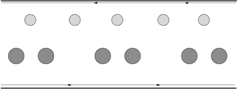
Figure 1: A system with $n$ quasihole pairs (held at pairs of anti-dots, depicted as shaded circles) supports $n$ qubits. Additional antidots (hatched) can be used to move the quasiparticles, as described in section III.

These qubits will be manipulated by braiding quasiparticles, which causes states in this $2^{n}$-dimensional Hilbert space transform into each other. To discuss these transformations, a different basis than (5) is useful. The effect of braiding quasiparticles is a combination of the explicit monodromy of the wavefunction and the Berry matrices obtained from adiabatic transport of the $\eta_{i}$s. The phase factors in (9) below have been chosen so that the latter are trivial and the former completely encapsulate quasiparticle braiding properties Nayak96c . (We could have worked with the basis ${\Psi_{(13)(24)}}$, ${\Psi_{(14)(23)}}$, in which there is no explicit monodromy, but then we would have to evaluate Berry matrix integrals Gurarie97 ; Tserkovnyak03 .)

$${\Psi^{(0,1)}}(z_{j})=\frac{\left({\eta_{13}}{\eta_{24}}\right)^{\frac{1}{4}}}{(1\pm\sqrt{x})^{1/2}}\,\left({\Psi_{(13)(24)}}\,\,\pm\,\,\sqrt{x}\,\,{\Psi_{(14)(23)}}\right)$$ (9)

where $\eta_{13}={\eta_{1}}-{\eta_{3}}$, etc. and $x~{}=~{}\eta_{14}\eta_{23}/\eta_{13}\eta_{24}$. (Note that we have taken a slightly different anharmonic ratio $x$ than in Ref. Nayak96c, in order to make (9) more compact than Eqs. (7.17), (7.18) of Ref. Nayak96c, .) From this expression, we see, for instance, that taking $\eta_{3}$ around $\eta_{1}$ transforms ${\Psi^{(0)}}(z_{j})$ into ${\Psi^{(1)}}(z_{j})$.

In the $2n$ quasihole case, the result can be stated as followsNayak96c ; Ivanov01 . The $2^{n}$ states of the system can be grouped into a representation of the Clifford algebra

$$\left\{{\gamma_{i}},{\gamma_{j}}\right\}=2\delta_{ij}$$ (10)

with $i,j=1,2,\ldots,2n$. We could, for instance, organize the states according to their eigenvalues ${\psi_{i}^{\dagger}}\psi_{i}=\pm 1$, where $\psi_{j}=\gamma_{2j-1}+i\gamma_{2j}$, $j=1,2,\ldots,n$. When quasiparticles $i$ and $j$ are exchanged, the states transform according toNayak96c ; Ivanov01 :

$$|\Psi\rangle\rightarrow e^{-\frac{\pi}{4}{\gamma_{i}}{\gamma_{j}}}|\Psi\rangle$$ (11)

These braiding matrices, $\tau_{ij}=\exp\left(-{\frac{\pi}{4}{\gamma_{i}}{\gamma_{j}}}\right)$ will be a set of topologically-protected unitary transformations which we can use to manipulate our qubits.

Several important calculational and heuristic tools follow from field theories for the Pfaffian state. While they illuminate this section and section III, they are somewhat technical and take us away from the main line of our exposition, so we have deferred a discussion of these field theories to appendix A. For reasons which are discussed there, it is convenient to call excitations which have the same braiding properties (up to Abelian phase factors) as, respectively, (a) the vacuum, (b) charge-$e/4$ quasiparticles, and (c) neutral fermions either $1,\sigma,\psi$ or, equivalently, isospin $0,\frac{1}{2},1$.

Thus far, we have assumed that the only quasiparticles in our system are the quasiparticles which we have induced on our anti-dots. There could also be thermally-excited quasiparticles. They are the main source of error and their density was estimated in ref. DasSarma05, to be exponentially small at low temperatures. However, even at zero temperature, there will always be some quasiparticles which are trapped by local variations in the potential, such as those cause by impurities. Assuming that they cannot move, the effect of these quasiparticles can always be accounted for with ‘software’, i.e. quantum computations must be done with some more complicated algorithms which compensate for the presence of these stray quasiparticles. As a practical matter, however, we would like to make them as benign as possible. To the extent that we can tune the magnetic field to the center of the plateau and use gates to move the edge of the system to avoid impurities (as in ref. Stern05, ), we should do so. If we can remove these localized quasiparticles with gate or a scanning probe microscope tip (such as an atomic-force microscope (AFM) tip) we should also attempt this. Finally, there is one simplifying feature of the Pfaffian state in particular, noted in refs. Stern05, ; Bonderson05, is that there is an even-odd effect with quasiparticles. An even number of quasiparticles fuse to form a quasiparticle with Abelian statistics, while an odd number of quasiparticles fuse to form a quasiparticle with non-Abelian statistics. Hence, we handle stray localized quasiparticles in the following way. We should associate each stray quasiparticle with one of the anti-dots (most naturally the anti-dot to which it is closest). Then, we want the number of stray quasiparticles associated with each anti-dot to be even. In this way, the degrees of freedom of the anti-dot are not modified by its associates. Finally, we need to ensure that the quasiparticle braiding trajectories always encircle an even number of stray quasiparticles. Then, as may be seem from repeated application of (11), the braiding matrices acting on the qubit Hilbert space are unaffected by the presence of the stray quasiparticles and the Hilbert space of the stray quasiparticles will not become entangled with it.

III Braiding and Interferometry

III.1 Braiding

The basic process by which we will manipulate many-quasiparticles states is the counterclockwise exchange depicted in Figure 2. We suppose that the quasiparticles are localized at anti-dots and that they are transferred from one anti-dot to another by varying the voltages on the anti-dots. With three anti-dots, an exchange can be performed. Two successive exchanges results in a full braid of one quasiparticle around the other. We may need to move one quasiparticle greater distances – for instance, to take it around several others – in which case we could use an array of anti-dots as a ‘bucket brigade’ (as in CCD devices such as digital cameras).

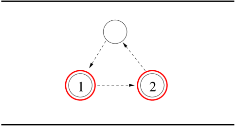
Figure 2: The exchange of two qubits through a third anti-dot.

The process depicted in Figure 2 can be used, for instance, to exchange a quasiparticle from one qubit with a quasiparticle from a different qubit. Such a process, which applies the gate $g_{3}$ ($g_{1}$ and $g_{2}$ will be introduced later) has a spacetime diagram which is depicted in Figure 14:

$${g_{3}}=\frac{1}{\sqrt{2}}\left(\begin{array}[]{cccc}1&0&0&-i\\ 0&1&-i&0\\ 0&-i&1&0\\ -i&0&0&1\end{array}\right).$$ (16)

This will be one of the basic gates used below.

One can imagine another possibility, which might become realistic at some point in the future: one quasiparticle could be dragged around another with a scanning probe microscope tip, e.g. an AFM tip, which could couple to a quasiparticle electrostatically with the required spatial resolution (which is presumably the magnetic length, on the order of 100 Å), as depicted in Figure 3.

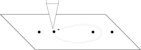
Figure 3: Using an AFM tip to braid quasiparticles.

There is one other type of braiding process which we can do, namely taking a quasiparticle from the edge of the system around one of the quasiparticles in a qubit, as depicted in Figure 4. Such an process is a NOT gate for this qubit.

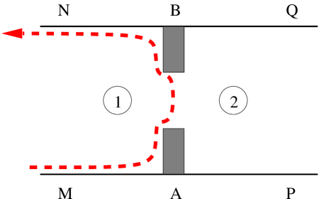
Figure 4: Taking a quasiparticle from the edge around one of the quasiparticles in a qubit implements a logical NOT on the qubit.

III.2 Interferometry

The basic process by which we will determine the state of our system, i.e. read our qubits, is an interference measurement. The two states of a qubit, which differ by the absence or presence of a neutral fermion $\psi$, can be distinguished by taking a charge $e/4$ quasiparticle around the pair. If the neutral fermion $\psi$ is present, an extra $(-1)$ occurs in the amplitude. In ref. DasSarma05, , it was shown how this minus sign could be detected by measuring the longitudinal resistance, $\sigma_{xx}$. It is determined by the probability for current entering the bottom edge from the left in Figure 5 to exit along the top edge to the left.

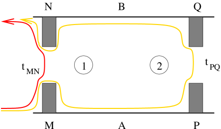
Figure 5: The state of a qubit can be determined from a measurement of the longitudinal conductance when inter-edge tunneling is allowed at two interfering junctions.

This is given, to lowest order in $t_{MN}$ and $t_{PQ}$, by the interference between two processes: one in which a ‘test’ quasiparticle tunnels from M to N; and another in which the ‘test’ quasiparticle instead continues along the bottom edge to P, tunnels to Q, and then moves along the top edge to N. (We subsume into $t_{PQ}$ the phase associated with the extra distance travelled in the second process and the extra Aharonov-Bohm phase.)

$$\sigma_{xx}\propto|t_{MN}|^{2}+|t_{PQ}|^{2}+2\text{Re}\left(t_{MN}{t_{PQ}^{*}}\left\langle\psi\left|B\right|\psi\right\rangle\right)$$ (17)

The third term is the interference between the two possible tunneling trajectories. $|\psi\rangle$ is the state of the qubit and the test quasiparticle, and $B$ is the operator which takes the test quasiparticle around the qubit, i.e. the braiding matrixFradkin98 . It can be computed by any of three equivalent ways: (1) taking $\eta_{3}$ around $\eta_{1}$ and $\eta_{2}$ in equation (9); (2) using the expression in (11); or (3) by evaluating the Jones polynomial at $q=e^{\pi i/4}$ for the link diagrams in Figure 6 (see appendix A for more on the meaning and evaluation of these diagrams). Either of these methods shows that $\left\langle\psi\left|B\right|\psi\right\rangle=\pm i$ for the two states of the qubit (the factor of $i$ comes from the Abelian sector of the theory). Hence,

$$\sigma_{xx}\propto|t_{MN}\pm i\,t_{PQ}|^{2}.$$ (18)

with the $+$ sign corresponding to the state $|0\rangle$ and the $-$ sign corresponding to the state $|1\rangle$.

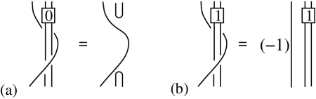
Figure 6: The interference between the two trajectories in Figure 5 can be obtained from the Jones polynomial (operator) evaluated on the two diagrams in this figure. In (a) the qubit is in the state $0$, while in (b) it is in state $1$.

In the many-qubit device of Figure 1, we would need tunnel junctions on either side of each qubit. By doing a sequence of tunneling conductance measurements, we could read each qubit in succession.

The presence or absence of a charge $e/4$ quasiparticle on an anti-dot can, of course, be detected simply by measuring the charge on the anti-dot. However, we will have occasion to measure the topological charge contained within some complicated spacetime loops, so it will also be useful to detect charge $e/4$ quasiparticles by interferometry. This can be done using the experimental setup of refs. Chamon97, ; Fradkin98, , as analyzed in refs. Stern05, ; Bonderson05, . When a charge $e/4$ quasiparticle is present on the anti-dot in Figure 7, the authors of refs. Stern05 ; Bonderson05 showed, the two trajectories do not interfere at all because $\left\langle\psi\left|B\right|\psi\right\rangle=0$ for equation (17) applied to this setup. This may be seen by evaluating the Jones polynomial at $q=e^{\pi i/4}$ for the first link in Figure 25 (see appendix A for more details). Hence, $\sigma_{xx}\propto{|{t_{1}}|^{2}}+{|{t_{2}}|^{2}}$. Varying the phases of $t_{1}$ and $t_{2}$ will not affect the longitudinal conductivity, which is the signature of a $\sigma$ particle.

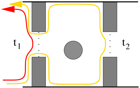
Figure 7: When there is a charge $e/4$ qusiparticle at the anti-dot in the middle of the device, then there is no interference between the two trajectories from $X$ to $Y$ contributing to the longitudinal conductance.

III.3 Tilted Interferometry

We now consider a generalization of the interferometry measurements of the previous subsection. Consider the diagram of Figure 8, in which a quasiparticle-quasihole pair is created, one member of the pair winds around another quasiparticle fixed at an antidot, and then the pair is again annihilated. This picture has a special feature, namely that the quasiparticle-quasihole loop can be continuously deformed into a single time slice or, for that matter, stretched out so that it takes place over a very long time, as in the third picture in figure 8. Because the antidot is simply sitting there passively, the evolution in the time direction can be chosen to our advantage.

Figure 8: A quasiparticle trajectory which winds around the antidot (straight line) can be deformed into a single time slice or stretched over a long time.

The amplitude for such a process is a measure of the total topological charge of the planar region bounded by this loop when deformed into a single time slice (as in the middle picture in Figure 8) – in other words, it measures the topological charge on the antidot. However, we are also free to consider such processes even when they do not have an interpretation in terms of the charge in some region of a fixed time-slice plane. This type of process can occur when the spacetime topology is non-trivial. For instance, if the system is on a torus, then there is a process in which a quasiparticle-quasihole pair is created, the quasiparticle taken around the meridian of the torus until it again meets the quasihole, and they are both annihilated. The corresponding loop does not enclose any region, so the usual interpretation is not available. Such loops are an important part of the Bravyi-Kitaev construction which we describe in section VI. An even more exotic possibility is depicted in Figure 9. Suppose we have two antidots which we bring close together so that they fuse for a short period of time $T$ before we pull them apart again. The spacetime diagram for this process is depicted in figure 9. Now consider a test quasiparticle which travels between the two dots. We have drawn two interfering trajectories which the test quasiparticle can take, labeled $p$ and $p^{\prime}$ in Figure 9. One of these trajectories, $p$, passes between the antidots before the merger while the other, $p^{\prime}$, passes between the anti-dots after the merger. The curve $\gamma$ captures the matrix element for the interference between these two trajectories.

Figure 9: Two antidots are merged for a short while and then separated again. The spacetime curve $\gamma$ encircles the merger region. The interference between the trajectories $p$ and $p^{\prime}$ measure the topological charge around this curve.

Ordinarily, one thinks of the amplitude of Figure 9 as being quite different from the middle one in Figure 8 (for instance, in Yang-Mills theory, a Wilson loop in the time direction is a measure of the force between separated charges, and therefore is a probe of confinement). However, in a topological phase, the curve $\gamma$ in Figure 9 is put on the same footing as the loop in Figure 8 (see appendix A for more on the relation between these diagrams and matrix elements in Chern-Simons theory). In a topological phase, the system does not know about any preferred metric (at least at long distances and low energies), so the time direction is just as good as a spatial direction. The results of such interferometry measurements correspond to topological charges, even though there isn’t an interpretation as the topological charge enclosed within a spatial loop. This may be familiar to some readers in the context Laughlin states in the quantum Hall effect. At $\nu=1/3$, an interference experiment around the meridian of a torus can return as its answer $q=0,\frac{1}{3},\frac{2}{3}$ (modulo $1$). Of course, the meridian of the torus does not enclose a region, so these are not charges enclosed within a meridional loop. Rather, these results correspond to the different possible quasiparticle boundary conditions (monodromies) around the meridian (namely $\psi\rightarrow e^{2\pi im/3}\,\psi$, $m=0,1,2$) which are the same as the phases which a quasiparticle would acquire in going around a region containing charges $q=0,\frac{1}{3},\frac{2}{3}$. Similarly, in the Pfaffian state tilted interferometry experiments will return as their result either $1,\sigma,\psi$, just as ordinary interferometry does.

Such measurements, in which quasiparticles encircle the time-dependent trajectories of quasiparticles on anti-dots, will be important for the protocols proposed in this paper, so it is worth spending a little time determining the limitations on such measurements, which we will call ‘tilted interferometry’ because the curve $\gamma$ cannot be deformed into a single time slice. (We thank Ady Stern for pointing out that tilted interferometry is analogous to the less well-known experiment proposed by Aharonov and Bohm Aharonov61 , in which the time dependence of $A_{0}$ affects quasiparticle interference between trajectories which do not pass through regions of finite electric (or magnetic) field.)

Unlike in the case of ‘ordinary’ interferometry, a tilted measurement cannot, strictly speaking, be a DC measurement. In an ordinary interference experiment, the different interfering quasiparticle wavefunctions are plane-wave-like states, hence, even though the travel time for the two trajectories in Figure 5 will be different, the wavefunctions will have spatio-temporal overlap, so they will still be able to interfere. Consider, however, the trajectories in Figure 9. Let us suppose that the two anti-dots are merged from time $t_{1}$ until time $t_{2}$. Then the first trajectory between the anti-dots must occur before $t_{1}$ while the second trajectory must occur after $t_{2}$. The only way that the wavefunctions for the two quasiparticle trajectories can have an overlap is if there is a delay built into the first trajectory which will allow the second one to ‘catch up’. This can be done as shown in Figure 10. We turn on and off some of the gates in order to direct the quasparticles along the specified trajectories. It will also be helpful to vary the quasiparticle velocities, as also shown in the figure.

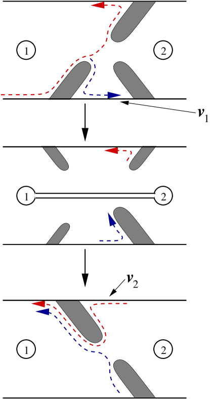
Figure 10: Two antidots are merged for a short while and then separated again. By putting delays into the possible quasiparticle trajectories (depicted in red and blue), we can enable them to interfere. In order to give the two anti-dots enough time to merge, we might wish to make the velocities ${v_{1}}$, ${v_{2}}$ small.

IV Topological Protection

The main advantage of using a topological state as a platform for quantum computation is that such states have intrinsic fault-tolerance Kitaev97 . The multi-quasihole states cannot be distinguished by local measurements, so long as the quasiholes are kept far apart. Hence, interactions with the environment, which are presumably local, cannot cause transitions between different topologically-degenerate states nor can it split them in energy. Suppose that we have $2n$ quasiparticles in our system, which is the device of Figure 1. One might worry, for instance, that there could be a local voltage fluctuation at one of the anti-dots. This has a trivial effect, however: the voltage fluctuation changes the energy of all $2^{n}$ states of our Hilbert space by precisely the same amount. Thus, it does not apply a phase gate, as could happen in a non-topological quantum computing scheme. The only way in which errors can occur is if a stray quasiparticle (created by the interaction with the environment) moves across the system and spontaneously performs a topological operation such as the braiding operation of Figure 4 or the interference measurement of Figure 5. This is closely related to the longitudinal resistance, which is the probability of an event in which a quasiparticle travels from one end of the system to another. If the spacing between anti-dots is large enough that quasiparticle transport at this scale is in the ohmic regime, then the error rate and the longitudinal resistance will be controlled by the same kind of processes. (We thank Leon Balents for a discussion of this point.) Experimentally, the longitudinal resistance is observed to be in the thermally-activated regime. Hence, it is limited by the density of thermally-excited quasiparticles, which is exponentially small $\exp(-\Delta/{k_{B}}T)$, where $\Delta$ is the quasiparticle energy gap and $T$ is the temperature. In ref. DasSarma05, , the resulting error rate $\Gamma$ was estimated to be

$$\frac{\Gamma}{\Delta}\sim\frac{{k_{B}}T}{\Delta}\,e^{-\Delta/{k_{B}}T}$$ (19)

In order to minimize the error rate, we want the temperature to be as low as possible, and we want the gap to be as large as possible, which seems to be aided by ultra-high mobility samples. The lowest temperature reached in the experiment of ref. Xia04, was $T=5\,{\rm mK}$, while the measured gap was $\Delta/{k_{B}}~{}=~{}0.5{\rm K}$. This leads to an error rate less than $10^{-30}$.

Of course, quasiparticles cannot be kept infinitely far apart, so there will be some splitting between multi-quasihole states. This splitting can be understood as the formation of a band of propagating Majorana fermion modes, which mix the localized states. The width of this band will be proportional to the tunneling matrix element between two quasiholes, which should decay as $w\sim e^{-R\Delta/c}$, for some constant $c$ with dimensions of velocity, where $R$ is the distance between quasiholes and $\Delta$ is the quasiparticle gap. The condition that the quasiparticles should be kept far apart can be translated into the statement that braiding operations should be done on time scales shorter than $1/w$. By keeping $R$ large compared to the inverse of the gap we can ensure that this will always be the case.

When quasiparticles are brought close together, however, there is no longer exponential protection. Suppose, for instance, that we merge two antidots into one large antidot of radius $\rho$. The splitting between the states $|0\rangle$ and $|1\rangle$ is now determined by processes in which a quasiparticle-quasihole pair is created at the edge of the antidot, they move in opposite directions around the antidot, and annihilate on the other side. Since there is no gap for the creation of quasiparticles at the edge of the antidot, there is no longer exponential suppression of such a process. Instead, it leads to a splitting $w\sim 1/\rho$. This means that the resulting phase error will be small if two quasiparticles are merged into a large antidot for a short period of time, even though the protection is not as good as exponential. However, there is still topological protection against bit flip errors since these would require a neutral fermion to tunnel to or from the qubit.

A second aspect of topological protection is the exactness of braiding operations. In the case of, say, spin qubits, gates are necessarily noisy because they depend on our ability to precisely tune the duration of a $\pi$ pulse or the strength of an applied magnetic field, which is necessarily imperfect. When gates are applied by braiding quasiparticles, however, no such tuning is necessary. The process is discrete: we either braid two quasiparticles or we don’t, and if we do braid them, then the corresponding unitary transformation occurs with the same level of exactness as the vanishing of the longitudinal resistivity or the quantization of the Hall resistivity.

However, one might wonder what happens if a quasiparticle only goes 359 degrees around another. If our qubits were quasiparticle pairs which we created out of the vacuum and then measured after annihilating them again in pairs at the end of the computation, then it would be clear that we would be dealing with closed braids. So long as the topological class of the closed braid traced out by the entire history of the system were preserved, it would not matter whether one quasiparticle went 360 degrees around another or only part of the way around. However, we envision measuring our qubits through a quantum interference measurement of the topological charge around some closed curves. Therefore, we will consider this issue in a little more detail. If one quasiparticle were to go 360 degrees around another then the initial and final states of the system lie in the same Hilbert space and the action of the braiding operation is just its unitary representative on this Hilbert space. However, if a particle only goes 359 degrees around another, then the initial and final states of the system do not lie in the same Hilbert space. Of course, the initial and final Hilbert spaces are unitarily equivalent, but the problem is that a unitary transformation between them could be trivial or it could undo the braiding operation. So what happens? The answer is that it depends on how the system is now measured. If the state of the system is measured by interference, then the result will depend on what path the interfering test quasiparticle takes (incidentally, this is always true since we can undo the effect of a braid by choosing a convoluted interfering path). If a particle goes 359 degrees around another, then almost all paths will give a result which is the same as if it had gone 360 degrees. In other words, it is not necessary to have very precise control of quasiparticle positions. Of course, if a quasiparticle were to only go 270 degrees around another, then we would have to exercise more care in choosing a trajectory for a test quasiparticle. However, even as drastic a deviation as this is not that serious a problem. The same caution holds if, instead of measuring the system, we wanted to act on it with yet another braiding operation. An example of such a situation is given in Figure 11. The same logic also holds for the uncontrolled motion of a stray quasiparticle; whether or not it has moved far enough to cause an error will depend on how the qubit is subsequently measured.

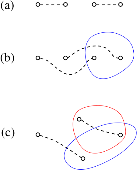
Figure 11: In (a), we have two pairs of quasiparticles. The dashed lines connect quasiparticles which fuse to form the (topologically) trivial particle. In (b), the second and third quasiparticles are exchanged. A measurement of the topological charge around the blue curve or an operation which takes another quasiparticle around this curve will give a non-trivial result as a result of this exchange. The same result is clearly obtained even if the final position of the quasiparticles is slightly different from those shown. If the exchange is incomplete, as in (c), then a measurement around the blue curve will give a non-trivial result but a measurement around the red curve will give a trivial result. So long as we are careful to measure the system with the blue curves in (b) and (c), we will find the correct result.

A potential second source of error is braiding operations which are performed too quickly. The time scale $t_{\rm op}$ over which a braiding operation is done must be slow compared to the gap, $t_{\rm op}\gg\Delta$. If this inequality is violated, a pair of quasiparticles might be created. These quasiparticles might then execute a non-trivial braid before annihilating each other (Coulomb blockade presumably prevents them from annihilating the quasiparticles on the anti-dots), thereby applying $g\cdot g^{\prime}$, for some $g^{\prime}$, rather than our intended gate $g$. The amplitudes for various $g^{\prime}$ depend on the ability of quasiparticles to move around the system (semiclassically, a random walk). To avoid such errors, we must make sure that such quasiparticles are not created in the first place by performing all braiding operations slowly, $t_{\rm op}\gg\Delta$. Again, it is advantageous to make the gap $\Delta$ as large as possible.

While the braiding operations and interference measurements described in this paper are similar in the sense that they both involve topological operations, they are actually quite different in an important respect. The braiding operations by which we envision manipulating our qubits are unitary operations. They involve moving quasiparticles around our system over time scales which must be long compared to the inverse of the gap and small compared to the inverse of the error rate:

$$\frac{1}{\Delta}\ll t_{\rm op}\ll T\,e^{\Delta/T}$$ (20)

So long as this order of time scales is respected and the quasiparticles are kept far apart (compared to the magnetic length, which is the only length scale in the problem), then the system is topologically-protected: the quantum state of the system evolves precisely as we specify.

On the other hand, our interference measurements are dissipative DC measurements (since they require non-zero $\sigma_{xx}$). As far as the multi-qubit Hilbert space is concerned, these are not unitary operations but, rather, projection onto specified states. It is worthwhile thinking a little more about how this ‘wavefunction collapse’ occurs because these measurements are potentially noisy. For instance, if a current-carrying edge quasiparticle should scatter inelastically, then the interference between its two possible trajectories will be spoiled. If this inelastic scattering rate becomes too large, then we will be unable to read the state of our quasiparticles through an interference measurement because we won’t be able to resolve two different values of the longitudinal conductivity. We would like to know when this will occur. Also, when this occurs, there is an interesting quantum measurement theory problem: does the qubit wavefunction still ‘collapse’ even when the inelastic scattering rate for the test particles is too high to allow us to distinguish the two states of the qubit?

To answer these questions, we begin by considering Figure 5. When a single test quasiparticle tunnels between the two edges (without scattering inelastically), its wavefunction becomes entangled with the state of the qubit: it is in one state, which we will call $|a\rangle$ when the qubit is in the state $|0\rangle$ and it is in a different state, $|b\rangle$, when the qubit is in the state $|1\rangle$. If the initial state of the system were $\alpha|0\rangle+\beta|1\rangle$, then it is now

$$\alpha|0\rangle|a\rangle+\beta|1\rangle|b\rangle$$ (21)

If $|a\rangle$ and $|b\rangle$ were the same, then there would be no entanglement with the test quasiparticle at all and the coherent superposition of $|0\rangle$ and $|1\rangle$ is maintained. However, if $|a\rangle$ and $|b\rangle$ were orthogonal, then the entanglement between the qubit and the test quasiparticle would completely spoil the coherent superposition of $|0\rangle$ and $|1\rangle$ (unless they can be disentangled later), i.e. the qubit wavefunction is ‘collapsed’.

For small tunneling amplitudes $t_{MN}$ and $t_{PQ}$, both $|a\rangle$ and $|b\rangle$ are concentrated on the bottom edge in Figure 5 and there is very little difference between these two states of the test quasiparticle. We can write

$$\langle b|a\rangle=1-\delta$$ (22)

with $\delta$ small. Hence, a single test quasiparticle does not do an effective job of ‘collapsing’ the qubit wavefunction. In order to be an effective measurement, we would like the qubit to be in the state $|0\rangle$ with probability $1$ when the test quasiparticle is in the state $|a\rangle$. When (22) holds, the qubit is instead in the state $\alpha|0\rangle+\beta(1-\delta)|1\rangle$ when test quasiparticle is in the state $|a\rangle$.

However, if $N$ test quasiparticles tunnel, then they all become entangled with the qubit. The combined state of the qubit and test quasiparticles is

$$\alpha|0\rangle|a,a,\ldots,a\rangle+\beta|1\rangle|b,b,\ldots,b\rangle$$ (23)

Notice that we now have

$$\langle b,b,\ldots,b|a,a,\ldots,a\rangle=(1-\delta)^{N}$$ (24)

For $N$ sufficiently large, these states are nearly orthogonal. Hence, the two states of the qubit cannot be coherently superposed unless the qubit is disentangled from the test quasiparticles. This cannot happen once the test quasiparticles leave the system at the current lead and thermalize there, which is an irreversible process. Thus, we conclude that the qubit wavefunction ‘collapses’: when the test quasiparticles are all in the state $|a\rangle$, the qubit is in the state $|0\rangle$ with probability $1-(1-\delta)^{2N}$, which is $\approx 1$ for $N$ large.

Now, consider the effect of inelastic scattering on the test quasiparticles. Those test quasiparticles which are inelastically scattered do not become entangled with the qubit. As far as measuring the qubit is concerned, we can forget about them. However, so long as there is a large number $N$ of quasiparticles which coherently encircle the qubit without inelastically scattering, the qubit wavefunction will collapse, according to the logic above. In principle, we can always ensure that this happens simply by waiting long enough, but once the inelastic scattering rate becomes of order $\Gamma_{\rm cr}\sim v/L$ where $L$ is the device size and $v$ the edge velocity, we would have to wait an exponentially long time.

The criterion for actually being able to read the value of the qubit is a little different, however. It depends on the resolution of our ohmmeter. When the inelastic scattering rate is too high, we won’t be able to resolve that there are actually two different values of the longitudinal conductivity. However, depending on how accurately we can measure the longitudinal conductivity, this could occur before the bound $\Gamma_{\rm cr}$ is reached. Thus, it is possible that the qubit wavefunction might ‘collapse’ by a measurement even though we would not be able to read the result.

We should conclude this section with a comment directed to our topologically-inclined readers (perhaps 100% of those who have come so far). Many critical details of the interferometer, such as the inelastic scattering length, travel times, quasiparticle ‘delays’, etc., are not topological in nature. How is this to be reconciled with the fact that in a topological theory all information on the change of state should be encoded by the $2+1$-dimensional spacetime history of the medium? The answer is that the topology of various tunneling trajectories gives us operators $h_{1}$, $h_{2}$, $\ldots$ evolving the system from initial to final states. However, experimental details determine other (dissipative) terms in the evolution equation of the density matrix of the system. In the limit that these other terms are small, a pure quantum state will remain pure and different $2+1$-dimensional space-time histories will contribute coherently to the evolution of this quantum state. When they are large, a pure quantum state will evolve into a mixed one and the $2+1$-dimensional space-time histories will effectively combine to form a super-operator for this mixed state density matrix.

V Universal Gate Set Using Some Topologically Unprotected Gates

For all of its remarkable properties, the Pfaffian state suffers from one serious drawback: the transformations generated by braiding operations are not sufficient to implement all possible unitary transformations Freedman02 ; BK . Hence, these operations do not permit universal quantum computation. However, we don’t need to supplement braiding with much in order to obtain a universal gate set. In this section, we explain a ‘quick and dirty’ way of doing this.

First, consider single-qubit operations. If we bring the two quasiparticles which comprise a qubit close together, as shown in Figure 12 then their splitting will become appreciable. This splitting has the form $\Delta\!E(r)\sim e^{-r\Delta/c}$, where $r$ is the distance between the quasiparticles and $c$ is some constant with dimensions of velocity. If we wait a time $T_{p}$ before pulling the quasiparticles apart again, then we will apply the phase gate:

$${U_{P}}=\left(\begin{array}[]{cc}1&0\\ 0&e^{i\Delta\!E(r)\,T_{p}}\end{array}\right)$$ (27)

A particularly convenient choice is $\Delta\!E(r)\,T_{p}=\pi/4$, which would allow us to apply the same transformation as the gate $g_{1}$ described in the next section.

Figure 12: By bringing together quasiparticles 1 and 2, which form a qubit, we can apply the gate $g_{1}$. This operation is unprotected and requires control of the distance between the quasiparticles and the length of time that they are brought together. However, the required precision might not be very stringent as a result of the availability of topologically-protected operations such as $g_{3}$.

Let us further assume that we can actually perform this operation on any pair of quasiparticles, not just two quasiparticles from the same qubit. Note that in order to do this we only need precise control over the distance between one pair of anti-dots since we can use $g_{3}$ to move any desired pair of quasiparticles to these preferred anti-dots (e.g. using the bucket brigade of auxiliary anti-dots to move quasiparticles). If we bring together in precisely the same manner two quasiparticles from different qubits, then we will couple the two qubits. In terms of the Majorana modes of (11), this gate is $\exp\!\left(\frac{\pi}{8}{\gamma_{i}}{\gamma_{j}}\right)$. (In the special case that $i$ and $j$ come from the same quasiparticle, this is the same as (27) up to an overall phase.)

The other gate which we need for universal quantum computation is the non-destructive measurement of the total topological charge of any pair of qubits. This can be done by using $g_{3}$ to move one qubit so that it is next to the other. Then, the interference measurement depicted in Figure 13 can determine the sum of the topological charges of the two neighboring qubits. This is a measurement of ${\gamma_{1}}{\gamma_{2}}{\gamma_{3}}{\gamma_{4}}$. According to ref. BK-fermions, , this measurement is equivalent to the application of the gate $\exp\left(\frac{\pi}{4}{\gamma_{1}}{\gamma_{2}}{\gamma_{3}}{\gamma_{4}}\right)$ so long as we have the ability to (a) create ancilla in the state $|0\rangle$ and (b) apply $\exp\left(\frac{\pi}{4}{\gamma_{i}}{\gamma_{j}}\right)$, which is simply the exchange of quasiparticles $i$ and $j$.

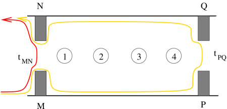
Figure 13: A non-demolition measurement of the total topological charge of two neighboring qubits (comprised of $1$, $2$ and $3$, $4$) can be done with the interference measurement shown here. Together with $g_{3}$ and the operation $U_{P}$ shown in Figure 12, this forms a universal gate set.

An obvious problem is that we have now given up some of the protection which we have worked so hard to obtain. Even if we could calculate $\Delta\!E(r)$ with high precision, there would always be some chance of a mistake in the length of time $T_{p}$ which the quasiparticles are close together. Thus, we would be in a situation in which some gates are exact – those resulting from braiding operations – while others are unprotected. The threshold error rate for the unprotected operations can be much less stringent (as high as $10\%$), as shown by Bravyi and Kitaev BK-magic for a specific set of perfect gates together with the noisy creation of a one-qubit ancilla in a specified state (a ‘magic state’). It is still an open problem what the threshold is for the set of protected gates and the one unprotected gate described above.

VI Bravyi-Kitaev Construction

In ref. BK, , Bravyi and Kitaev constructed a universal set of gates for a system in the topological phase described by $SU(2)_{2}$ Chern-Simons theory, which is the effective field theory Fradkin98 ; Fradkin99 likely to describe the $\nu=5/2$ quantum Hall state, apart from an Abelian factor which is unimportant here. For reference, their gates $\{g_{1},g_{2},g_{3}\}$ are:

$${g_{1}}=\left(\begin{array}[]{cc}1&0\\ 0&e^{\pi i/4}\end{array}\right)\,,{\hskip 14.22636pt}{g_{2}}=\left(\begin{array}[]{cccc}1&0&0&0\\ 0&1&0&0\\ 0&0&1&0\\ 0&0&0&-1\end{array}\right),$$ (34)

$$\textnormal{and }\>{g_{3}}=\frac{1}{\sqrt{2}}\left(\begin{array}[]{cccc}1&0&0&-i\\ 0&1&-i&0\\ 0&-i&1&0\\ -i&0&0&1\end{array}\right).{\hskip 42.67912pt}$$ (39)

$g_{1}$ is a phase gate on a single qubit. $g_{2}$ and $g_{3}$ are two-qubit gates. $g_{2}$ is a controlled phase gate: if both qubits are in state $|1\rangle$, the state acquires a $(-1)$. Otherwise, it is unchanged. Alternatively, if we change the basis of the second qubit to $(|0\rangle\pm|1\rangle)/\sqrt{2}$, then $g_{2}$ is simply a CNOT gate. $g_{3}$ is a two-qubit gate which, together with $g_{1}$, $g_{2}$ form a universal gate set. This particular gate is chosen because it can be implemented with the simple quasiparticle braiding process depicted in Figure 14.

Figure 14: Quasiparticles 1 and 2 form a qubit; 3 and 4 form a second qubit. Exchanging 2 and 3 applies the gate $g_{3}$.

The controlled phase gate $g_{2}$ is more complicated. Suppose we have two qubits composed of two pairs of quasiparticles (1,2) and (3,4). We would like to multiply the state of the system by $(-1)$ only when qubits $(1,2)$ and $(3,4)$ are both in state $|1\rangle$. The problem is that if qubit $(3,4)$ is in state $|1\rangle$ and we take it around quasiparticle $1$, then a factor of $(-1)$ results, regardless of whether $(1,2)$ is in the state $|0\rangle$ or $|1\rangle$. The trick of Bravyi and Kitaev BK is to split qubit $(1,2)$ in such a way as to produce a charge $e/4$ quasiparticle only when $(1,2)$ is in the state $|1\rangle$. If this occurs, then we can take $(3,4)$ around this quasiparticle, and a $(-1)$ will occur if $(3,4)$ is also in the state $|1\rangle$.

In order to do this, we perform the following steps which we will describe here without regard to their feasibility (which will be taken up in the next section). Suppose that quasiparticles $1$ and $2$ are at antidots, which should be understood as punctures in the quantum Hall fluid. The state of the $(1,2)$ qubit is equal to the topological charge around the loop $B_{0}$ in the top diagram in Figure 15. We will denote this topological charge by $W\!({B_{0}})$. We create an overpass which connects these two punctures, as depicted in the middle part of Figure 15. We check with an interferometry measurement that the boundary of the antidots-plus-overpass, labeled $B_{1}$ in Figure 15, has trivial topological charge, $W\!({B_{1}})=1$. If it doesn’t, we break the overpass and rebuild it again until we find $W\!({B_{1}})=1$. We don’t need to repeat this very often since the probability for $W\!({B_{1}})=1$ is $1/2$ and the probability for $W\!({B_{1}})=\psi$ is also $1/2$ (since the isospin $0$ and $1$ quasiparticles have the same quantum dimension – i.e. the same zero-temperature entropy per particle – in $SU(2)_{2}$ Chern-Simons theory). Each time we break the overpass, we return the qubit to its original state. This follows from the general principle (see appendix B) that adding quantum media is reversible simply by deleting what was added (whereas deleting quantum media is generally irreversible).

Once we know that $W\!({B_{1}})=1$, it follows for reasons which we discuss below that if $(1,2)$ is in state $|1\rangle$ (i.e. if $W\!({B_{0}})=\psi$) then $W\!({C})=\sigma$ in figure 15. If this is the case, then taking $(3,4)$ around the loop $C$ multiplies the state by $(-1)$ if $(3,4)$ is in state $|1\rangle$ and leaves it unchanged if it is in state $|0\rangle$. On the other hand, if $(1,2)$ is in state $|0\rangle$, then $W\!({C})=(1-\psi)/\sqrt{2}$ in Figure 15, and taking $(3,4)$ around $C$ doesn’t change the state. Therefore, this sequence of operations applies the gate $g_{2}$ of (34).

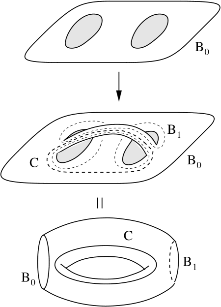
Figure 15: By adding an overpass, we connect two antidots. The dashed curve labeled $B_{1}$ is the combined boundary of the antidots-plus-overpass. In the implementation of both $g_{1}$ and $g_{2}$, we need to check that $W\!({B_{1}})=1$. In the case of $g_{2}$, the controlled qubit must be taken around $C$ in order to implement a controlled phase gate on it. To enact $g_{1}$, a double Dehn twist must be performed in $C$. The two anti-dots joined by an overpass in the middle of the figure are topologically equivalent to a torus with two punctures corresponding to $B_{0}$ and $B_{1}$ as shown at the bottom. The meridian of the torus is $C$.

The Chern-Simons theory calculations which lead to this result are facilitated by the observation that the topology of two anti-dots joined by an overpass is a torus with two punctures, corresponding to $B_{0}$ and $B_{1}$, as depicted in the bottom diagram of Figure 15. The curve $C$ is the meridian of the torus. Once we have made sure that $W\!({B_{1}})=1$, we know that we can fill in this puncture without changing anything; in other words, the system is equivalent to a torus with one puncture, $B_{0}$. Observe that $W\!({B_{0}})$ is the state of the qubit: it is either $1$ or $\psi$. We would now like to determine $W\!({C})$. This can be obtained from the $S$-matrix of the theory, which relates the topological charge around the meridian, $W\!(M)$, to the topological charge around the longitude, $W\!(L)$. If $W\!({B_{0}})$ is $1$, the $S$-matrix is,

$$S^{1}_{ij}=\left(\begin{array}[]{ccc}\frac{1}{2}&\frac{1}{\sqrt{2}}&\frac{1}{2}\\ \frac{1}{\sqrt{2}}&0&-\frac{1}{\sqrt{2}}\\ \frac{1}{2}&-\frac{1}{\sqrt{2}}&\frac{1}{2}\\ \end{array}\right)\,,{\hskip 8.5359pt}i,j=1,\sigma,\psi.$$ (43)

However, $W\!(L)$ is simply the topological charge on each of the antidots, which is $\sigma$, (i.e. $(0,1,0)$ in the matrix notation of (43)). Hence, the $S$-matrix tells us that $W\!({C})$ is the linear combination $(1-\psi)/\sqrt{2}$. On the other hand, if $W\!({B_{0}})=\psi$, then the vanishing of all $S$-matrix elements $S^{\psi}_{ij}$ other than $S^{\psi}_{\sigma\sigma}=e^{-i\pi/4}$ tells us that $W\!({C})=\sigma$.

We now turn to $g_{1}$. The first step in the implementation of gate $g_{1}$ in (34) is the same as above: we take the two anti-dots associated with the qubit under consideration and join them with an overpass as in Figure 15. Again, we check that $W\!({B_{1}})=1$. Now, however, we act on this qubit by performing a double Dehn twist on the curve $C$. This means that we cut along the curve $C$, thereby forming two boundaries. We rotate one of them by $4\pi$ relative to the other (i.e. perform two twists) and then glue them back together. Finally, we remove the band, thereby returning the system to a state of two $\sigma$ quasiparticles, one on each of the two anti-dots.

A Dehn twist on $C$ has an equivalent effect as a $2\pi$ rotation of the topological charge associated with $C$. Since the conformal spins of $1$, $\sigma$ and $\psi$ are, respectively, $0$, $\frac{1}{16}$, and $\frac{1}{2}$, the effect of performing two successive Dehn twists is simply the identity ${1^{2}}=(-1)^{2}$ if $W\!({C})$ is, respectively, $1$ or $\psi$ and it is ${\left(e^{2\pi i/16}\right)^{2}}=e^{\pi i/4}$ if the topological charge is $\sigma$. Since $W\!({C})$ is perfectly correlated with the value of the qubit, the effect of this sequence of operations is the gate $g_{1}$ in (34). Note that a single Dehn twist would necessarily change the charge of the two anti-dots by transferring charge $e/4$ from one to the other.

VII From Non-Planar Topology to Time-Dependent Planar Topology

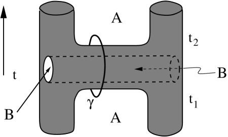
Figure 16: A non-planar overpass configuration can be mimicked by breaking the region $A$ and adding $B$. This is done by merging the two anti-dots between times time $t_{1}$ and $t_{2}$. During this merger interval, we allow the quantum Hall fluid the fill the region $B$. This faux pass splits the merged anti-dot in the perpendicular direction. These changes are then undone to return the system to its initial configuration. In order to verify that removing $A$ was harmless, we have to perform a tilted interferometry measurement to check that the topological charge around $\gamma$ is trivial. See Figure 20 for a time slicing of this process.

The operations described in the previous section may never be practical in a real quantum Hall device. Overpasses with high mobility are implausible, let alone gating them in and out at will. Dehn twists seem an even more remote possibility. Fortunately, there are some features of Chern-Simons theory, which is the effective field theory of our system, which can be exploited to mimic these types of operations without leaving the plane or attempting to perform surgery on our quantum Hall fluid. In this section, we will explain these features of Chern-Simons theory and how they can be used to apply the gates $g_{1}$ and $g_{2}$. Once this problem in topological quantum field theory (TQFT) has been solved, we turn in the next section to the new set of problems which arises when we try to realize this construction in a quantum Hall device. For the reader who is uninterested in the TQFT details and wishes to skip ahead to the next section, we summarize the results of this section: (1) an operation equivalent to the addition and removal of an overpass between two antidots can be performed by connecting the two antidots so long as a curve surrounding the connection (which might be tilted) has trivial topological charge; (2) a measurement of the topological charge around a curve $\gamma$ (with a particular framing) is equivalent to a ‘Dehn filling’ on this curve (which, in turn, is related to a Dehn twist, as explained below) modulo a few caveats described in this section. With these two observations in hand, we can replace ‘impossible’ operations with operations which are merely very difficult. In section VIII, we give concrete illustrations of how this can be done with the device architecture described in this paper.

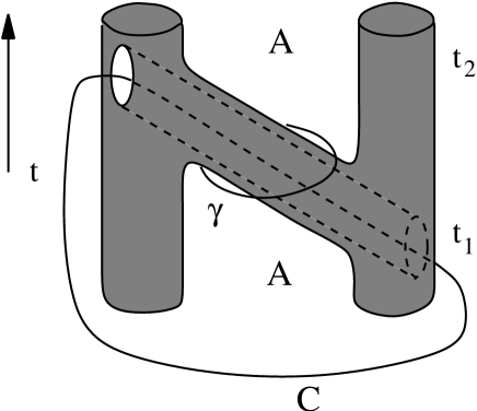
Figure 17: Topologically, the process depicted here is equivalent to that depicted in Figure 16. However, as a result of the tilt of the faux pass, the triviality of the charge around the hole in $A$ can be measured with an untilted measurement. Consequently, the curve $\gamma$ can now be deformed into a single time slice. The curve labelled $C$ in this figure is equivalent to the curve $C$ which goes over the overpass in Figure 15. This is the curve on which we wish to perform a Dehn twist. Measuring the topological charge around this curve allows us to effect the same transformation on the quantum state of the system without any surgery. See Figure 24 for a time slicing of this process.

One particularly fortuitous feature of topological field theories, for our purposes, is the fact that when the topological charge around a hole is trivial, then the part of the system outside the hole is impervious to whether the hole is filled in or not. For example, if the topological charge around $\gamma$ in Figure 9 is trivial, then this spacetime history is equivalent, as far as a topological field theory is concerned, with a spacetime history in which there is no merger whatsoever between the two anti-dots. This suggests a way in which we can effectively have overpasses by taking advantage of the time direction so that ‘over’ is realized as ‘at a different time’, as shown in Figure 16. Suppose we want a band of material $B$ to form an overpass over another band $A$. We instead break $A$ at time $t_{1}$, allow $B$ to pass, use $B$ for whatever purpose, break $B$, and then reconstitute $A$ at time $t_{2}$. If we could measure the topological charge around the resulting time-like hole ${t_{1}}<t<{t_{2}}$ in $A$ and if we found that it was trivial, it would be, as far as Chern-Simons theory were concerned, as if $A$ were never broken. The faux overpass – or, simply, faux pass – $B$ is then just as good as an overpass.

Note that this figure can be continuously deformed to our convenience. From a topological point of view, Figure 16 is equivalent to Figure 17. However, their realizations are quite different, and they have different practical advantages and disadvantages. The tilted measurement of $\gamma$ in Figure 16 is untilted in Figure 17. However, Figure 17 has a moving anti-dot and island (whose velocity is the slope of the faux pass in Figure 17).

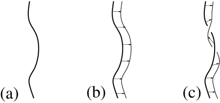
Figure 18: The curve in (a) can be framed, for example, as shown in (b) and (c). The self-linking number in (c) is greater by $+1$ than in (b).

A second ‘impossible’ operation which we need to perform is a Dehn twist on a closed curve $C$. In order to make it possible, we use the following two facts. (i) It is a fundamental identity of the “Kirby calculus” that $(-1)-$framed ‘Dehn surgery’ on a simple linking circle imparts a $(+1)$ Dehn twist and, of course, a double Dehn twist arises if two such surgeries are performed. By ‘frame’, we mean that the curve $C$ is thickened into a ribbon so that a self-linking number can be well-defined: it is the linking number of the two curves formed by the edges of the ribbon (one edge of the ribbon is $C$, the other edge is traced out by the tip of the frame vector). Some examples of framed curves are shown in 18. We would like $C$ to be framed so that this self-linking number is $(-1)$. The meaning of ‘Dehn surgery’ is that a tubular neighborhood (in spacetime) of the loop $C$ is deleted and then glued back so that the meridian disk is glued to the circle defined by the tip of the frame vector. Obviously, physical limitations prevent us from doing this in a quantum Hall device, but we can instead (ii) measure the particle content of a loop $\zeta$ in the interior of a $2+1-$dimensional space-time. If the result is $1$, we have (up to an overall normalization factor, corresponding to capping a $2-$sphere) accomplished Dehn surgery on $C$ as far as Chern-Simons theory is concerned. This Dehn surgery on a spacetime history has the result of making it into a history which interpolates between an initial state before a Dehn twist has been performed on the faux pass and a final state in which the faux pass has been Dehn twisted.

We would like to explain the relation between Dehn twist, Dehn surgery, and Dehn filling. Dehn twist is a method for constructing a diffeomorphism of a surface: given a closed loop $l$ on a surface, cut the surface along $l$, twist one side by $2\pi$ and reglue. This is either a $+$ or $-$ Dehn twist (depending on sign conventions). Our interest in Dehn twist is that it provides a way to transform a 3-manifold $M$ by cutting it open along a surface and then regluing using a Dehn twist. To discuss this procedure, we will simplify matters by concentrating on an annular neighborhood $A$ of $l$. (The framing of $l$ defines an annulus $A$, as may be seen in figure 18b,c.) We split the 3-manifold $M$ along $A$, thereby opening a toridal cavity within $M$. The boundary of this cavity is a torus $B$ which is just two copies of $A$, joined along their boundaries. This new manifold with the cavity is essentially $M\backslash\text{neigh}(l)$, $M$ minus a neighborhood of $l$. The term “Dehn filling” refers to gluing a solid torus back into the cavity; the double process of first making the cavity and then refilling it is called “Dehn surgery”. The possible outcomes of Dehn surgery are parameterized by the slope of that curve on the cavity boundary $B$ which is matched to the disk factor $D^{2}$ of the reglued solid torus ${D^{2}}\times{S^{1}}$. Notice that Dehn twist, from one copy of $A$ to the other, carries a radial arc in one copy to a twisted arc in the other so that the two mate together to become a diagonal – either (1,1) or (1,-1) in the natural $B$-coordinates (the first component counts the winding number around the “meridian” or shortest direction and the second coordinate counts the winding number around the “longitude” defined by either component of the boundary of $A$ within $B$) depending on whether the Dehn twist is $+$ or $-$ respectively. Conversely, the instuction to do “$-1$ Dehn surgery on $l$” can be expressed as: 1. open the cavity around $l$ (a normal framing on $l$ is required at this point to pick out the surface $A$) 2. change the correspondence between the two copies of A by a $+1$ Dehn twist. 3. with respect to these new coordinates, Dehn fill the solid torus by gluing the disk to the meridian of the cavity. (Steps 2 and 3 together constitute $-1$ Dehn filling since they tell us to match the $(1,-1)$ curve on the cavity boundary $B$, which is taken to the meridian by step 2, to the disk within the reglued solid torus.) Thus cutting and regluing by a $+/-$ Dehn twist is identical to doing $+/-$ Dehn surgery. The later is simply a more three-dimensional language for the former. Measuring the trivial charge along a curve $C$ is, from the point of view of Chern-Simons theory, equivalent to supplying a disk (containing no quasiparticles) for the curve $C$ to bound, or an entire solid torus (with no Wilson loop at its core) for $B$ to bound. Thus, we propose to accomplish through measurement a topological operation, namely Dehn twist, which otherwise would have no reasonable experimental realization.

An important detail to be considered is that measurement might result in a nontrivial charge. This means, in fact, that the reglued solid torus does carry a Wilson loop of precisesly that charge. This Wilson loop is depicted in figure 19 as a loop $\beta$ in the exterior solid torus, as shown. These states with Wilson loops correspond to the other two ground states on the torus (up to an additional factor of $2$ degeneracy coming from the Abelian part of the theory). These are the states obtained by performing the Chern-Simons functional integral over a solid torus with a Wilson loop carrying topological charge ($\sigma$ or $\psi$ resp.), but expressed in the meridinal basis.

$$\Psi[a]=\int_{A_{|T^{2}}=a}D\!A\,\,{W}[A,\beta]\,e^{{\int_{M}}\cal{L}_{\rm CS}[A]}$$ (44)

where $\cal{L}_{\rm CS}[A]$ is the Chern-Simons Lagrangian and $M={D^{2}}\times{S^{1}}$ is the solid torus. $W[A,\beta]$ is the Wilson loop (i.e. the trace of the holonomy of the gauge field $A$), $W[A,\beta]={\rm Tr}\left({\cal P}\exp({\oint_{\zeta}}A)\right)$, with the trace taken in the fundamental or the adjoint representation (for, respectively, $\sigma$ or $\psi$), and the functional integral is over $SU(2)$ gauge fields $A$ such that $A=a$ on $T^{2}$, the boundary of the solid torus. Since the Wilson loop must be around the meridian, $\beta$ is depicted as ‘outside’ the torus in figure 19.

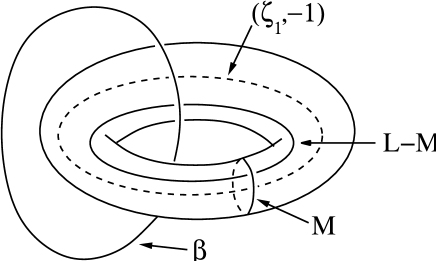
Figure 19: If we measure the topological charge around $({\zeta_{1}},-1)$ and it is not $1$, then we have performed a Dehn filling on $({\zeta_{1}},-1)$ and left behind a Wilson loop $\beta$, carrying this topological charge, inside the solid torus. The state of the system is given by the functional integral in equation (44) for this manifold. The $3D$ mapping cylinder of a Dehn twist can be described as: delete a solid torus, then replace it with a twisted Dehn filling. For convenience, we have drawn the torus in a non-standard way so that $L-M$ appears simple.

In order to perform a double Dehn twist on $C$, we need to measure the topological charge around two framed curves which run parallel to $C$. We will call these curves $(\zeta_{1},-1)$ and $(\zeta_{2},-1)$; the $-1$ denotes the framing. Note that $C$ is equivalent to untwisted copies of the $\zeta$’s, which can be denoted $(\zeta_{1},0)$ and $(\zeta_{2},0)$. In order to measure the topological charge around $(\zeta_{1},-1)$ and $(\zeta_{2},-1)$, our measurement quasiparticles will have to go along a curve with an extra twist; a way of realizing this is shown in Figure 23. If a measurement finds $W\!({\zeta_{1}})=1$, then we have performed the desired Dehn twist. Finding $W\!({\zeta_{1}})=\psi$ isn’t the end of the world because the extra Wilson loop which results just gives some extra minus signs. However, we want to avoid $W\!({\zeta_{1}})=\sigma$. One way to do this is to take a charge $\sigma$ around the loop $(\zeta_{1},0)$. Then let $({\zeta_{1}},-1)$ run parallel to the charge, encircling it to yield the framing $(-1)$. In Figure 23, we have depicted a time-slicing of such a framed curve: the measurement quasiparticle must wind around the quasiparticle which is following the loop $(\zeta_{1},0)$.

We can now use a similar argument to that used after (43) to show that $W\!({\zeta_{1}})=(1-\psi)/\sqrt{2}$: since $(\zeta_{1},-1)=L-M$ (i.e. longitude - meridian), we claim that $W\!({\zeta_{1}})$ is given by $ST^{-1}|\sigma\rangle$ where n

$${S}=\left(\begin{array}[]{ccc}1/2&\sqrt{2}/2&1/2\\ \sqrt{2}/2&0&-\sqrt{2}/2\\ 1/2&-\sqrt{2}/2&1/2\end{array}\right)\textnormal{ and }{T}=\left(\begin{array}[]{ccc}1&0&0\\ 0&e^{i\pi/8}&0\\ 0&0&-1\end{array}\right)$$

in the $\{1,\sigma,\psi\}$ basis. We check that $ST^{-1}\,\,|\sigma\rangle~{}=~{}e^{-i\pi/8}\,(|1\rangle~{}-~{}|\psi\rangle)/\sqrt{2}$. Hence, a measurement of $W\!({\zeta_{1}})$ can only give $1$ or $\psi$ (with equal probabilities). By doing this with another charge, parallel to $\zeta_{2}$ and encircled by it, we can force a measurement of $W\!({\zeta_{2}})$ to be $1$ or $\psi$, again with equal probabilities, and completely independent of the result of the $W\!({\zeta_{1}})$ measurement.

To see that $ST^{-1}$ gives the correct transformation, note that we wish to transform from the longitudinal basis $L$ to the framing $=k$ basis, $L+kM=$ longitude $+k$(meridian). To define a basis $V(T^{2})=\sum_{\text{particle types,}a}V_{a\overline{a}}(S^{1}\times I)$, we need to select a circle, the “cuff”, to cut the torus along a dual circle, the “seam”, to trivialize the resulting annulus as $S^{1}\times I$. The transformation is then done in the following two stepsWalker91 :

$$\text{(cuff, seam)}=\\ (L,M)\stackrel{{\scriptstyle\textnormal{twist}{{}^{k}}}}{{\longrightarrow}}(L,M+kL)\stackrel{{\scriptstyle S^{-1}}}{{\longrightarrow}}(M+kL,L).$$ (45)

Hence, the composition of these transformations is given by: $S^{-1}T^{k}S$.

In the discussion above, we have shown that with two tilted interferometry measurements, we can accomplish the same thing as a double Dehn twist, as far as Chern-Simons theory is concerned, with the caveat that extra Wilson loops might be added to to the final state.

One important difference between the Bravyi-Kitaev protocol BK and our proposal to mimic this with time-dependent planar topologies is that, in the latter case, $W({B_{1}})$ cannot be measured until the end of the entire operation. Consequently, we must use the overpass without knowing if $W({B_{1}})=1$ or $\psi$ (these are the only two possibilities since two $\sigma$s can only fuse into these two possibilities). This means that we must learn to live with the possibility that $W({B_{1}})=\psi$. The saving grace is that we will at least know after the operation whether $W({B_{1}})=1$ or $\psi$, which allows us to compensate in the latter case. Under the assumption that $W({B_{1}})=1$, we deduced from the $S-$matrix of the theory that $W\!({C})$ is perfectly correlated with $W\!({B_{0}})$, which is the value of the qubit.

$$W\!({B_{0}})=1 \Rightarrow W\!({C})=(1-\psi)/\sqrt{2}$$ (46)

$$W\!({B_{0}})=\psi \Rightarrow W\!({C})=\sigma$$ (47)

However, the same logic shows that if $W\!({B_{1}})=\psi$, then

$$W\!({B_{0}})=1 \Rightarrow W\!({C})=\sigma$$ (48)

$$W\!({B_{0}})=\psi \Rightarrow W\!({C})=(1-\psi)/\sqrt{2}$$ (49)

In other words, the correlation between $W\!({C})$ and $W\!({B_{0}})$ has been reversed or, in other words, the roles of the states $1$ and $\psi$ of the qubit have been reversed.

In the case of $g_{2}$, this applies to the control qubit, on which all of the operations are performed (the controlled qubit is passive). Hence, if we find at the end of our procedure that $W\!({B_{1}})=1$, then we know that we have applied the desired phase gate $g_{2}$. If , instead, $W\!({B_{1}})=\psi$, then the gate has inadvertently interchanged the roles of $1$ and $\psi$ within the controlling qubit so that

$${\tilde{g}_{2}}=\left(\begin{array}[]{cccc}1&0&0&0\\ 0&-1&0&0\\ 0&0&1&0\\ 0&0&0&1\end{array}\right)$$ (54)

has instead been applied. This is not too serious since repeated application of the protocol gives a random walk in the group $Z_{2}\bigoplus Z_{2}=\{1,{g_{2}},{\tilde{g}_{2}},{g_{2}}{\tilde{g}_{2}}\}$. Our $W\!({B_{1}})$ measurements tell us where we are within $Z_{2}\bigoplus Z_{2}$ as we randomly walk; we simply halt upon reaching $g_{2}$. The tails on a “long walk” decay exponentially so this delay is acceptable.

Now consider $g_{1}$. Let us first suppose, for simplicity, that $W\!(\zeta_{1})=W\!(\zeta_{2})=1$. If we find at the end of our procedure that $W\!({B_{1}})=1$, then we know that we have applied ${g_{1}}=\left(\begin{smallmatrix}1&0\\ 0&e^{\pi i/4}\end{smallmatrix}\right)$. However, if we find that $W\!({B_{1}})=\psi$, then we have applied

$$\left(\begin{array}[]{cc}e^{\pi i/4}&0\\ 0&1\end{array}\right)=e^{\pi i/4}\>g_{1}^{-1}.$$ (57)

There is one added complication in the case of $g_{1}$, as compared to $g_{2}$: we have the added uncertainty in the outcome of the $W\!(\zeta_{1})$, $W\!(\zeta_{2})$ measurements. If $W\!(\zeta_{1})=W\!(\zeta_{2})=\psi$, then two Wilson loops carrying $\psi$ appear within the solid torus. However, these two Wilson loops fuse to form $1$, which is again trivial, just as in the case $W\!(\zeta_{1})=W\!(\zeta_{2})=1$. However, if $W\!(\zeta_{1})\cdot W\!(\zeta_{2})=\psi$, which is as good as a single Wilson loop $\zeta$ carrying topological charge $\psi$ parallel to $C$, there can be a non-trivial effect. If $W\!({C})=(1-\psi)/\sqrt{2}$, which means that $W\!({B_{0}})\cdot W\!({B_{1}})=1$, the Wilson loop contributes no extra phase. However, if $W\!({C})=\sigma$, which means that $W\!({B_{0}})\cdot W\!({B_{1}})=\psi$, then the Wilson loop $\zeta$ encircles the same topological charge $\sigma$ which is encircled by $C$ (to which it is parallel). When a $\psi$ encircles a $\sigma$, a $(-1)$ results. This means that if $W\!(\zeta_{1})\cdot W\!(\zeta_{2})=\psi$, then instead of $g_{1}$ or $g_{1}^{-1}$, we have acutally applied ${\sigma_{z}}\,{g_{1}}=g_{1}^{-3}$ or ${\sigma_{z}}\,g_{1}^{-1}=g_{1}^{3}$, where ${\sigma_{z}}=\left(\begin{smallmatrix}1&0\\ 0&-1\end{smallmatrix}\right)$.

In all eight measurement outcomes for $W\!(\zeta_{1})$, $W\!(\zeta_{2})$ we have, up to an overall phase, implemented either $g_{1}$, $g_{1}^{-1}$, $g_{1}^{-3}$, or $g_{1}^{3}$. Thus our protocol generates a type of random walk on $Z_{8}$. Since we know the measurement outcomes we may iterate the protocol until we arrive at $g_{1}$, which is again efficient.

Therefore, we conclude that finding $W\!({B_{1}})=\psi$ is not a calamity for the implementation of either $g_{1}$ or $g_{2}$.

VIII Realizing the Bravyi-Kitaev Gates with Time-Dependent Planar Topology and Tilted Interferometry

In this section, we will discuss how the operations of the previous section, which are merely difficult, rather than impossible, might be implemented in a quantum Hall device. We need to be able to do four things: (1) move our qubits at will, (2) create ‘faux passes’ – which are equivalent to overpasses in Chern-Simons theory – with the spacetimes histories depicted in Figure 16 or Figure 17, (3) measure the topological charge around a tilted trajectory such as $C$ in Figure 17, and (4) create a quasiparticle pair and move them around as desired before annihilating them. We have already discussed (1) and (3) in section III. We now turn to (2) and (4).

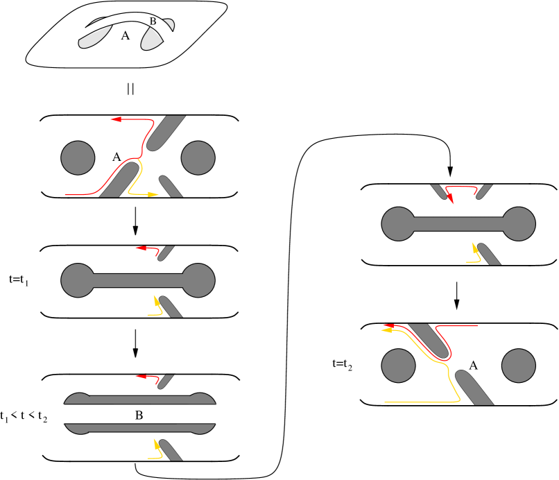
Figure 20: A non-planar overpass configuration can be mimicked by breaking the region $A$ and adding $B$. This is done by merging the two anti-dots at time $t_{1}$ and splitting them in the other direction. The faux pass $B$ is then used to either apply $g_{1}$ or $g_{2}$, as described in Section VII. These changes are then undone to return the system to its initial configuration. In order to verify that removing $A$ was harmless, we have to perform a tilted interferometry measurement in which the red and yellow trajectories interfere.

The spacetime history shown in Figure 16 can be realized by the sequence of steps depicted in Figure 20. In this figure, the region $A$ (the ‘underpass’) of the quantum Hall fluid separates the two anti-dots. At time $t_{1}$, region $A$ is broken so that the two anti-dots are joined into one large oblong anti-dot. After this occurs, a strip of quantum Hall fluid is allowed to split the large anti-dot in the perpendicular direction (the bottom left picture in Figure 20). This is the faux pass $B$ which plays the role of the overpass. The spacetime region carved out by this strip is the tube in Figure 16.

In order to check that the topological charge around the time-like hole is trivial, we need to do a tilted interferometry measurement similar to that depicted in figures 9, 10. The interference between the red and yellow curves in Figure 20 measures the topological charge around the hole in $A$. There is an obvious drawback here, which is that the result of this measurement will not be know until after the entire procedure is complete. We will return to this issue later. For now, let us consider the other operations which we need to perform.

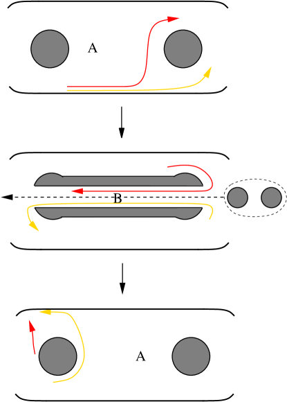
Figure 21: The interference between the red and yellow trajectories is a measurement of the topological charge around $B_{1}$. In order to apply $g_{2}$, we take the controlled qubit across the faux pass

During the time that the faux pass region $B$ is available, we must take our qubit over it and then check whether the topological charge around the curve $B_{1}$ is $1$ or $\psi$. These are both depicted in Figure 21. Both of these processes must occur while those depicted in Figure 20 are simultaneously occurring. We envision doing both of these with a bucket brigade of anti-dots which are used to ferry both the measuring test quasiparticles and the controlled qubit across the faux pass, as shown in Figure 22. This is relatively straightforward for the qubit: the two quasiparticles comprising the qubit must be moved across the region $B$ in figure 20. Of course, this process must occur without the two quasiparticles of the controlled qubit fusing. Hence, we need to keep them far apart, either with a large faux pass or by having one follow at a distance behind the other.

The test quasiparticle with which we measure $B_{1}$ is trickier. Consider the red and yellow trajectories in Figure 21. There should be some small amplitude $t_{r}$ for a quasiparticle at the bottom edge to tunnel to the top edge via the red trajectory, which takes it over the faux pass, and a small amplitude $t_{y}$ for it to tunnel via the yellow trajectory. In the ‘bucket brigade’ scenario, the red trajectory is actually composed of a series of hops from one anti-dot to another. Let us assume that the amplitude for a quasiparticle to hop from the edge onto the first anti-dot is $t_{1}$. Let us further assume that the amplitude for it to hop from the first anti-dot to the second anti-dot is $t_{bb}$; from the second to the third, again $t_{bb}$; and so on until the quasiparticle finally hops onto the top edge. Then ${t_{r}}\sim{t_{1}}\,t_{bb}\,t_{bb}\ldots t_{bb}$, where the number of factors of $t_{bb}$ depends on how many anti-dots are in the bucket brigade. We need this amplitude to be small so that the topological order of the state is not degraded, but is should be large enough to be measurable. This might be most easily done by making $t_{1}$ small and $t_{bb}$ not too small. Of course, the same reasoning holds for the yellow trajectory. Finally, we need the amplitudes for these two processes to interfere coherently. This means that the coherence time for a quasiparticle on either one of these trajectories must be longer than the time of flight, which might be difficult to ensure.

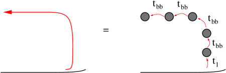
Figure 22: The quasiparticle trajectories shown in Figures 20 and 21. may actually look more like the trajectory on the right above: a series of hops from one small anti-dot to another.

In order to implement $g_{1}$, we need to also send an auxiliary quasiparticle over the faux pass. This can be done as shown in Figure 23, perhaps using a ‘bucket brigade’, as in Figure 22. We must then measure the topological charge around the curve $({\zeta_{1}},-1)$, which means that we must measure the interference between the trajectories in Figure 23. We do this with $({\zeta_{2}},-1)$ in the same way.

There is a problem with the procedure described in these figures, which is that the configuration shown in the third picture in Figure 20 has two anti-dots merged. Consequently, the state of the two anti-dots does not have exponential protection. The splitting between the two states of the qubit formed by this pair of anti-dots is $w\sim 1/x$, where $x$ is the linear extent of the merged antidot. This can actually be avoided in the following way. Instead of merging the two anti-dots, we send an intermediary which shuttles from one to the other. This is done by breaking the anti-dot on the right into two anti-dots, one with electrical charge $e/4$ and the other with no electrical charge. We then move the neutral anti-dot to the left and merge it with the left anti-dot. This would simply replace the merger by the ‘tilted merger’ shown in Figure 17. In order to have an overpass, we need the anti-dot to be annular so that there is a region of $\nu=5/2$ quantum Hall fluid in the middle of it, as shown in Figure 24. While this moving shuttle is between the two anti-dots, we check by ordinary interferometry that it carries topological charge $1$, rather than $\psi$. If it doesn’t, then we re-merge it with the right anti-dot and repeat the same process until we find that the topological charge around the shuttle is $1$. The abortive attempts at this do not affect the qubit (except possibly by an irrelevant overall phase): splitting $a$ into $b\otimes c$ and then re-fusing results in the original particle type, so it is a multiple of the identity. The qubit is clearly unaffected since the phase resulting from such operations is independent, by locality, of the state of the qubit. In order to apply $g_{2}$, the controlled qubit must sit in the interior of the shuttle as it moves from one anti-dot of the control qubit to the other. In order to apply $g_{1}$, the auxiliary quasiparticles must do so. It must be noted that this approach again has the difficulty that the coherence times of complicated interfering quasiparticle trajectories must be kept long.

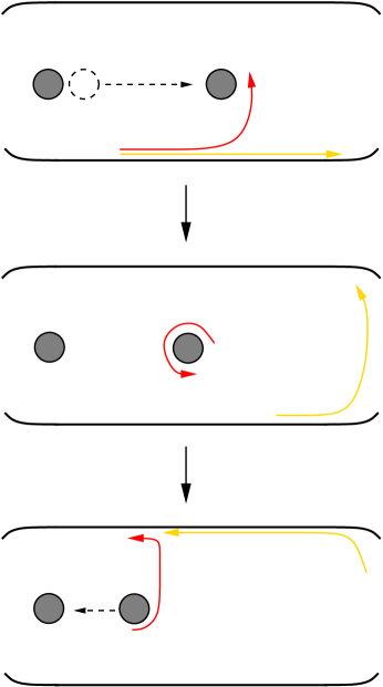
Figure 23: In order to apply $g_{1}$, we must create a pair of auxiliary quasiparticles, take one over the faux pass (not shown), and then annihilate them again. While this is occurring, we must measure the topological charge around a curve which follows the auxiliary quasiparticle over the faux pass, while encircling it. By encircling the auxiliary quasiparticle (presumably while hopping along a bucket brigade of anti-dots), this trajectory obtains a non-trivial framing: it is the framed curve $({\xi_{i}},-1)$. A measurement of the interference between the red and yellow curves can determine the topological charge around this (tilted) framed curve.

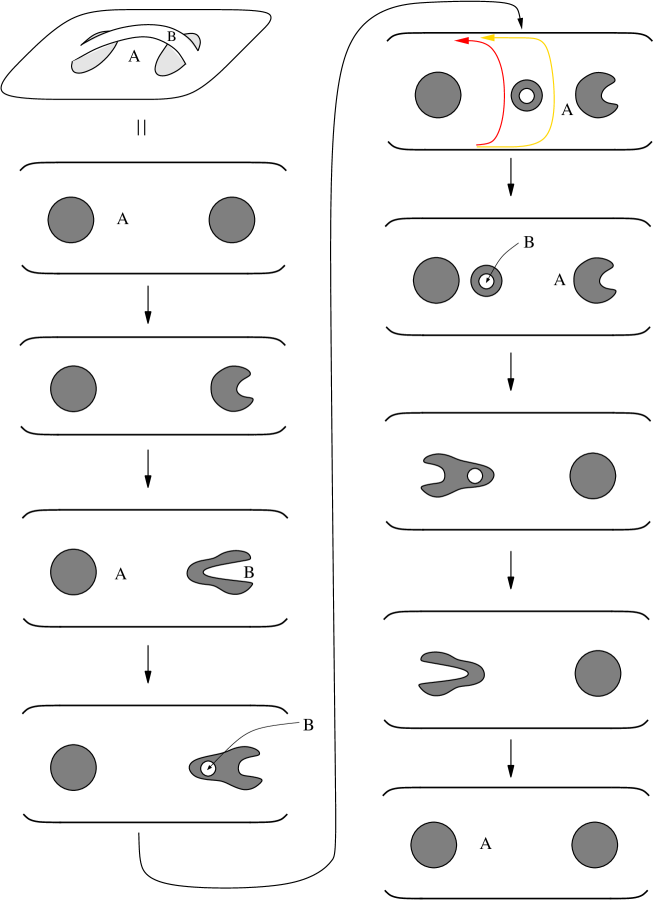
Figure 24: By sending an annular intermediary between the two anti-dots, we can construct the spacetime history of Figure 17. The shuttle between the two antidots is annular and the island of quantum Hall fluid in the middle of the annulus is the faux pass $B$. A measurement of the interference between the red and yellow trajectories can check that the tilted hole in region $A$ is topologically trivial as far as Chern-Simons theory is concerned.

IX Discussion

In this paper, we have discussed how the $\nu=5/2$ quantized Hall plateau can be used as the basis of a quantum computer, assuming that this plateau is in the universality class of the Pfaffian state. Pairs of charge $e/4$ quasiparticles form qubits. We propose to pin the quasiparticles at anti-dots so that by moving the anti-dots, we move the quasiparticles. The two states of a pair of quasiparticles, $|0\rangle$ and $|1\rangle$, can be identified with the primary fields $1$, $\psi$ of the conformal field theory of the critical $2D$ Ising model, or with the spin $0$ and spin $1$ representations of $SU(2)_{2}$ Kac-Moody algebra (or the related quantum group). The value of any qubit can be read by a transport measurement which is sensitive to the interference between two possible quasiparticle trajectories encircling the qubit. However, local measurements cannot distinguish the two states of the qubit so long as the two quasiparticles are kept apart. The error rate is astronomically low, so these qubits form an essentially perfect quantum memory DasSarma05 . Two simple gates can be implemented by quasiparticle braiding: (1) tunneling a quasiparticle from the edge between the two quasiparticles comprising a qubit and (2) by exchanging a quasiparticle from one qubit with a quasiparticle from another qubit.

In order to be able to apply any possible unitary transformation to our qubits – i.e. in order to have universal quantum computation – we can try either of two approaches. One is to use the unprotected operation of bringing together the two quasiparticles comprising a qubit so that a phase gate will result from the resulting energy splitting between their two states. Although this operation is unprotected, the error threshhold may not be too strict because the other operations are exact due to topological protection. The other approach is to use some complicated manipulations of the anti-dots which involves moving, splitting, and rejoining them in order to fool the topological field theory governing the Pfaffian state into behaving as if we have performed non-embeddable topology changes. Although complicated, these operations allow, in principle, for a universal set of exact gates. By now the reader may have decided that the former approach is more promising in the short run because it does not require extremely complicated quasiparticle manipulations. However, if technological advances make the latter approach more feasible, then it has the virtue of complete topological protection. Also, the beautiful topology involved lends it an intrinsic ‘coolness’ factor.

If the weaker $\nu=12/5$ plateau proves to be a non-Abelian state related to $SU(2)_{3}$ Chern-Simons theory, then neither of these two compromises would be necessary. We would again realize qubits as above, but, in this case, the braid group alone would be sufficient for universal quantum computation.

Appendix A Effective Field Theory approach to the Pfaffian State

The multi-quasihole structure which we encountered in section II is precisely the same structure as occurs in the Ising model. Indeed, the motivation of Moore and Read for first writing down the Pfaffian wavefunction was its relation to conformal blocks of the Ising modelMoore91 . The first hint that there might be such a connection comes from the observation that the Pfaffian factor in the wavefunction (1) is equal to a correlator of $\psi$ fields:

$$\left\langle\psi({z_{1}})\,\psi({z_{2}})\,\ldots\,\psi({z_{2n}})\right\rangle={\rm Pf}\!\left(\frac{1}{z_{j}-z_{k}}\right)$$ (58)

Multi-quasihole wavefunctions are related to conformal blocks with spin fields such as Moore91 ; Nayak96c . Before discussing this in any more detail, however, we should first explain why the quasiparticles of the Pfaffian state have anything to do with the primary fields of the Ising model.

The answer lies in the connection discovered by Witten Witten89 between $2+1$-D Chern-Simons theories and $1+1$- or $2$-D conformal field theories (CFTs). According to Witten Witten89 (see also the explicit constructions of Elitzur et al. Elitzur89 ), the Hilbert space of states of a Chern-Simons theory on a $3D$ manifold $M=X\times R$ is equivalent to the vector space of conformal blocks of an associated CFT on the $2D$ manifold $X$. The Hilbert space of a Chern-Simons theory with sources located at ${\bf r_{1}},{\bf r_{2}},\ldots,{\bf r_{n}}$ carrying representations ${\rho_{1}},{\rho_{2}},\ldots,{\rho_{n}}$ is equivalent to the conformal blocks of an $n$-point correlation function of primary fields associated with these representations.

If we have an electron system which is described at long-wavelengths by a Chern-Simons theory, we can use the wavefunctions of the Chern-Simons theory with sources as approximate wavefunctions of the electron system. By the above connection, this means we can use conformal blocks in the associated CFT as wavefunctions of the electron system. In each of these two steps, the essential features which are preserved are the braiding properties of the quasiparticles of the system. The different primary fields in the CFT correspond to the different topological charges in the Chern-Simons theory, which, in turn, correspond to the different quasiparticle species in the electron system.

As shown in ref. Fradkin98, ; Fradkin99, , the low-energy effective field theory associated with the Pfaffian state of bosons at $\nu=1$ is an $SU(2)_{2}$ Chern-Simons theory. The effective field theory for fermions at $\nu=1/2$ (or other even-denominator filling fractions and for bosons at other odd-denominator filling fractions) is a deformation of this theory: a Higgs-ed $SU(2)_{2}$ Chern-Simons theory (independent of the filling fraction) coupled to a $U(1)$ Chern-Simons theory with a filling-fraction-dependent coupling constant. The CFT corresponding to this Chern-Simons theory is the tensor product of an $SU(2)/U(1)$ coset model with a $c=1$ $U(1)$ factor Moore91 . However, the $SU(2)/U(1)$ coset model is equivalent to the Ising model. According to this correspondence, the primary fields which are associated with half-flux quantum quasiparticles are Ising spin fields (multiplied by a field from the $c=1$ sector).

The $U(1)$ factor, which accounts for the charge, gives the correct Abelian factors for quasiparticle statistics and contributes a factor to the ground state degeneracy. The more non-trivial physics is contained in the $SU(2)$ part of the theory. Hence, we can be a little sloppy and drop their $U(1)$ quantum numbers and refer to quasiparticles by their $SU(2)_{2}$ quantum numbers (which we will call ‘isospin’). According to this nomenclature, there are three primary fields, with isospins $0,\frac{1}{2},1$, corresponding to $1,\sigma,\psi$ of the Ising model. These are, respectively, the vacuum, the half-flux quantum quasiparticle, and the neutral fermion. The topological degeneracy of multi-quasiparticle states reflects the decomposition of the product of two isospin $1/2$s: $\frac{1}{2}\otimes\frac{1}{2}=0\oplus 1$. Thus, there are two different reasons why it is natural to call the two states of a qubit $0$ and $1$.

Returning now to the conformal blocks which model wavefunctions of electrons at $\nu=1/2$ (in the first excited Landau level), we note that the corresponding CFT contains both the $c=1/2$ Ising model and a $c=1$ chiral boson (accounting for the electrical charge):

$${\cal S}=\int{d^{2}}z\,\left(\psi\,{\partial_{\overline{z}}}\psi+({\partial_{z}}\phi)({\partial_{\overline{z}}\phi})\right)$$ (59)

We retain only the right-handed part $\varphi$ of $\phi=\varphi+{\overline{\varphi}}$, with ${\partial_{\overline{z}}}\varphi={\partial_{z}}{\overline{\varphi}}=0$. If we assume that the operator corresponding to the electron is:

$$\Psi_{\rm el}(z)=\psi(z)\,e^{i\varphi(z)\sqrt{2}}$$ (60)

then we have

$$\left\langle\Psi_{\rm el}({z_{1}})\,\Psi_{\rm el}({z_{2}})\,\ldots\,\Psi_{\rm el}({z_{2N}})\,e^{\int{d^{2}}z\rho\,\varphi(z)\sqrt{2}}\right\rangle=\\ \prod_{j<k}(z_{j}-z_{k})^{2}\prod_{j}e^{-|z_{j}|^{2}/4}\cdot{\rm Pf}\!\left(\frac{1}{z_{j}-z_{k}}\right)~{}.$$ (61)

The last term in the correlation function on the left-hand-side of this equation is a neutralizing charge background without which the Coulomb gas correlation function would vanish. To find the primary fields of this $c=3/2$ theory, we need to put together the primary fields of the (right-handed chiral component of the) Ising model – the identity, $1$; the Ising spin field, $\sigma$; and the Majorana fermion, $\psi$ – with exponentials of the chiral boson $\varphi$. The primary fields must be local with respect to the electron operator – i.e. quasiparticles can have non-trivial statistics with each other but they must have trivial statistics with respect to an electron since an electron wavefunction must be single-valued in electron coordinates. A field which satisfies this condition is

$$\Phi_{\rm qp}(\eta)=\sigma(\eta)\,e^{i\varphi(\eta)/2\sqrt{2}}$$ (62)

This field corresponds to the charge $e/4$ quasiparticle:

$$\biggl{\langle}\Phi_{\rm qp}({\eta_{1}})\Phi_{\rm qp}({\eta_{2}})\,\times\\ \Psi_{\rm el}({z_{1}})\Psi_{\rm el}({z_{2}})\ldots\Psi_{\rm el}({z_{2N}})\,e^{\int{d^{2}}z\rho\,\varphi(z)\sqrt{2}}\biggr{\rangle}=\\ {\rm Pf}\!\left(\frac{\left({z_{j}}-{\eta_{1}}\right)\left({z_{k}}-{\eta_{2}}\right)+{z_{j}}\leftrightarrow{z_{k}}}{z_{j}-z_{k}}\right)\,\times\\ \prod_{j<k}(z_{j}-z_{k})^{2}\prod_{j}e^{-|z_{j}|^{2}/4}$$ (63)

The four-quasihole wavefunctions in (9) are given by the conformal blocks of $\langle\Phi_{\rm qp}\Phi_{\rm qp}\Phi_{\rm qp}\Phi_{\rm qp}\Psi_{\rm el}\Psi_{\rm el}\ldots\Psi_{\rm el}\,\exp({\int{d^{2}}z\rho\,\varphi\sqrt{2}})\rangle$. The two different wavefunctions correspond to the two different fusion channels $\sigma\cdot\sigma\sim 1+\psi$. (Furthermore, the two conformal blocks are the wavefunctions (9) in the special basis in which the explicit monodromy of the wavefunction gives the complete braiding matrices Gurarie97 ).

The full set of primary fields is given in the table below. The columns correspond to Ising model primary fields while the rows correspond to the $c=1$ primary fields. The entries of the table are the quasiparticle electrical charges. Each quasiparticle corresponds to an operator formed by multiplying the operator at the top of its column by the operator to the left of its row. Note that it is not a naive tensor product between the two theories because the quasiparticles containing $\sigma$ are offset by $e^{i\varphi/2\sqrt{2}}$ from those containing $1,\psi$. (Again, these assignments are determined by the requirement of locality with respect to the electron operator (60).)

    $1$    $\sigma\,e^{i\varphi/2\sqrt{2}}$     $\psi$ $1$ 0 $e/4$ 0 $e^{i\varphi/\sqrt{2}}$ $e/2$ $3e/4$ $e/2$

One of the nice features of the relationship between the Pfaffian state and $SU(2)_{2}$ Chern-Simons theory is that it allows us to use Witten’s remarkable result relating Chern-Simons theory and the Jones polynomial of knot theory Witten89 . Braiding matrix elements can be obtained by computing the Jones polynomial of the corresponding link diagrams Fradkin98 ; DasSarma05 ; Bonderson05 . For instance, the qubit-flipping property of the process which takes $\eta_{3}$ around $\eta_{1}$ in (9) can be obtained by evaluating the Jones polynomial (operator) at $q=e^{\pi i/4}$ for the links in Figure 25.

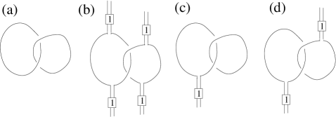
Figure 25: By evaluating the Jones polynomial at $q=\exp(\pi i/4)$ for these links, we can obtain the desired matrix elements for braiding operations manipulating the qubit. The boxed $1$ is a projector on the pair of quasiparticles which puts them in the state $|1\rangle$.

What do these pictures mean and how are they evaluated? They are essentially Feynman diagrams for the topological interactions of quasiparticles. The lines in this picture represent isospin $1/2$ quasiparticles. Since the electric charge is not accounted for in these diagrams, quasiparticles and quasiholes are identical as far as these diagrams are concerned. (The electric charge just contributes Abelian phase factors.) If two of these isospin $1/2$ quasiparticles fuse to form a spin $0$, then they can annihilate to give the vacuum. Otherwise, they fuse to form an isospin $1$ particle, which we denote by a boxed $1$ on the two lines (as in Figure 25b, for example). Consider, for instance, the spacetime trajectories of the test quasiparticle and the quasiparticle on the antidot in Figure 7. They will look like Figure 26a.

Figure 26: (a) A quasiparticle trajectory which winds around a quasiparticle at an antidot (b) a quasiparticle trajectory which doesn’t wind around the antidot; (c) the matrix element between the states resulting from these two trajectories.

In this figure, we assume that a quasiparticle-quasihole pair is created at $P$ and the quasiparticle goes around the antidot. The other trajectory, with which this interferes, is depicted in figure 26b: in this case, the test quasiparticle does not go around the antidot. The interference term between these two processes, i.e. the third term in equation 17, is given by the matrix element between these two processes, depicted in Figure 26c. It is just Figure 26b inverted (which corresponds to turning a ket into a bra) and then stacked on top of 26a. This matrix element measures the topological charge associated with the loop in Figure 26c.

Hence, to summarize: we specify an initial state $|{\psi_{0}}\rangle$ of $n$ qubits by drawing $2n$ incoming lines, which are grouped into $n$ pairs. At the bottom of the diagram (the distant past), each pair is either created from the vacuum (in which case this qubit is in the state $|0\rangle$) or was fused to form an isospin $1$ particle (in which case this qubit is in the state $|1\rangle$). The final state $|\psi\rangle$ is obtained by braiding these quasiparticles, which is depicted in the figure with the vertical direction on the page being positive time. Finally, the matrix element between $|\psi\rangle$ and another state $|\chi\rangle$ is obtained by inverting the corresponding diagram for $|\chi\rangle$ and stacking it on top of the diagram for $|\psi\rangle$, connecting each quasiparticle line from $\langle\chi|$ to the corresponding quasiparticle line from $|\psi\rangle$.

The matrix element associated with such a diagram is evaluated recursively in the following way. Each diagram is replaced by the sum of two diagrams both of which have one fewer crossing according to the rule:

$$\pspicture[0.4](28.45274pt,28.45274pt){\psset{linewidth=1.0pt}\psbezier(9.48424pt,0.0pt)(9.48424pt,14.22636pt)(18.96849pt,14.22636pt)(18.96849pt,28.45274pt)}{\psset{linewidth=1.0pt}\psbezier(18.96849pt,0.0pt)(18.96849pt,9.48424pt)(17.07164pt,11.38109pt)(17.07164pt,12.80373pt)}{\psset{linewidth=1.0pt}\psbezier(11.38109pt,15.649pt)(11.38109pt,17.07164pt)(9.48424pt,18.96849pt)(9.48424pt,28.45274pt)}\endpspicture\>=\>q^{1/2}{\hskip-5.69046pt}\pspicture[0.4](28.45274pt,28.45274pt){\psset{linewidth=1.0pt}\psbezier(9.48424pt,0.0pt)(9.48424pt,14.22636pt)(9.48424pt,14.22636pt)(9.48424pt,28.45274pt)}{\psset{linewidth=1.0pt}\psbezier(18.96849pt,0.0pt)(18.96849pt,14.22636pt)(18.96849pt,14.22636pt)(18.96849pt,28.45274pt)}\endpspicture\;+\;q^{-1/2}{\hskip-5.69046pt}\pspicture[0.4](28.45274pt,28.45274pt){\psset{linewidth=1.0pt}\psbezier(9.48424pt,0.0pt)(9.48424pt,9.48424pt)(18.96849pt,9.48424pt)(18.96849pt,0.0pt)}{\psset{linewidth=1.0pt}\psbezier(18.96849pt,28.45274pt)(18.96849pt,18.96849pt)(9.48424pt,18.96849pt)(9.48424pt,28.45274pt)}\endpspicture$$ (64)

The new diagrams come with corresponding coefficients as indicated in the above relation. We continue this procedure until all crossings are eliminated. The projector on the isospin $1$ state is replaced by the explicit expression:

$$\pspicture[0.4](28.45274pt,28.45274pt){\psset{linewidth=1.0pt}\psline(9.48424pt,0.0pt)(9.48424pt,8.53581pt)}{\psset{linewidth=1.0pt}\psline(9.48424pt,19.91692pt)(9.48424pt,28.45274pt)}{\psset{linewidth=1.0pt}\psline(18.96849pt,0.0pt)(18.96849pt,8.53581pt)}{\psset{linewidth=1.0pt}\psline(18.96849pt,19.91692pt)(18.96849pt,28.45274pt)}{\psset{linewidth=1.0pt}\pspolygon(7.11317pt,8.53581pt)(21.33955pt,8.53581pt)(21.33955pt,19.91692pt)(7.11317pt,19.91692pt)}\uput[u](14.22636pt,6.2596pt){$1$}\endpspicture\>=\>\pspicture[0.4](28.45274pt,28.45274pt){\psset{linewidth=1.0pt}\psbezier(9.48424pt,0.0pt)(9.48424pt,14.22636pt)(9.48424pt,14.22636pt)(9.48424pt,28.45274pt)}{\psset{linewidth=1.0pt}\psbezier(18.96849pt,0.0pt)(18.96849pt,14.22636pt)(18.96849pt,14.22636pt)(18.96849pt,28.45274pt)}\endpspicture\>-\;\frac{1}{d}{\hskip-5.69046pt}\pspicture[0.4](28.45274pt,28.45274pt){\psset{linewidth=1.0pt}\psbezier(9.48424pt,0.0pt)(9.48424pt,9.48424pt)(18.96849pt,9.48424pt)(18.96849pt,0.0pt)}{\psset{linewidth=1.0pt}\psbezier(18.96849pt,28.45274pt)(18.96849pt,18.96849pt)(9.48424pt,18.96849pt)(9.48424pt,28.45274pt)}\endpspicture$$ (65)

where $d=-q-q^{-1}$. Finally, every closed loop is given the value

$$\pspicture[0.4](28.45274pt,28.45274pt){\pscircle(14.22636pt,14.22636pt){9.48424pt}}\endpspicture=\>d$$ (66)

Appendix B The effect of adding or deleting bands of material to a topological state

In this appendix, we discuss how a $\nu=5/2$ fractional quantum Hall droplet is modified by topology change, in particular when bands of material are added or deleted. The basic guideline is that adding a band of material does not change the state of the system, so it is reversible; deleting a band of material can cause the state of the system to change irreversibly.

In the Bravyi-Kitaev construction discussed in section VI, we described a process in which a band of material (the overpass in the middle picture in Figure 15) is added and then later removed. The spacetime history of such a process is depicted in Figure 27. In this figure, two $\sigma$ quasiparticles on anti-dots fuse to form $1$ or $\psi$, which is the topological charge of the boundary. The spacetime history of the quantum Hall droplet with two anti-dots is shown as a ‘pair of pants’ legs $P\times I$, where $P$ is the disk with two punctures and $I$ is the interval of time $[0,1]$. The spacetime history depicting the addition and subsequent removal of an overpass connecting the anti-dots is a handle connecting the two pants legs. The union of this $1$-handle and the spacetime history of the droplet with two anti-dots is $W=P\times I\cup(1-\text{handle})$.

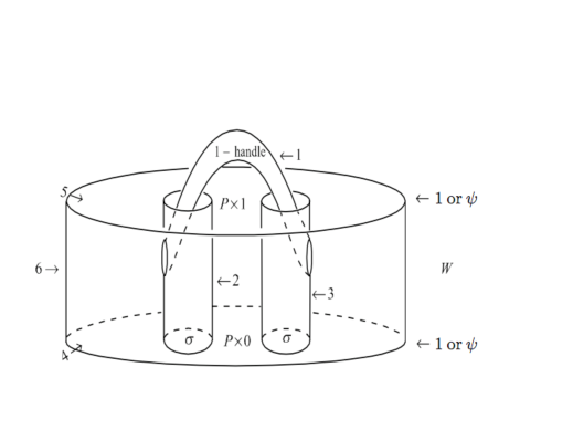
Figure 27: The spacetime history of a process in which an overpass connecting two antidots is added and then removed. Warning: this history does not embed in $2+1$ dimensions, so the $z-$coordinate in this picture cannot be literally interpreted as time. The handle must move into a fourth direction.

We would like to check that this procedure leaves invariant the qubit supported by $P$ (rather than, say, applies a phase gate). In order to do this, we imagine evaluating the Chern-Simons functional integral on the $3$-manifold $W$. It will give a state in the Hilbert space of the boundary $\partial W$. However, this boundary is divided into subsurfaces by loops bounding specified topological charges, so the Hilbert space of the boundary is, in fact, the tensor product of the Hilbert spaces of the subsurfaces. Hence, $W$ specifies a vector $\psi_{1}$ in: $V_{0,0}\otimes V_{0,\sigma,\sigma}\otimes V_{0,\sigma,\sigma}\otimes V_{\sigma,\sigma,x}\otimes V_{\sigma,\sigma,x}^{\ast}\otimes V_{x,x}$, where the factors come from subsurfaces $1,\ldots,6$ in Figure 22. The zero label in the first three factors is dictated by the presence of disks in $W$ capping the boundary of the first component (a cylinder). The gluing axiom Walker91 ; Turaev00 tells us that removing the $1-$handle determines a canonical isomorphism to $Z(P\times I)$ carrying $\psi_{1}$ to $\psi_{0}$ in $V_{0}^{\ast}\otimes V_{0}\otimes V_{0,\sigma,\sigma}\otimes V_{0,\sigma,\sigma}\otimes V_{\sigma,\sigma,x}\otimes V_{\sigma,\sigma,x}^{\ast}\otimes V_{x,x}$. After supplying the canonical base vectors $\beta_{0}^{\ast}\in V_{0}^{\ast},\beta_{0,\sigma,\sigma}\in V_{0,\sigma,\sigma}$ and $\beta_{x,x}\in V_{x,x},\psi_{1}$ is canonically identified with id $\in$ Hom $(V_{\sigma,\sigma,x})\cong V_{\sigma,\sigma,x}^{\ast}\otimes V_{\sigma,\sigma,x}$. Note that no $x-$dependent phase has entered the calculation. Thus we have proved, in the abstract language of TQFTs, that adding and then breaking a band induces the identity operator on the qubit supported in $P$.

The situation is rather different if, instead, we cut out a band to join the internal punctures and then restore it (i.e. fuse the internal punctures and then separate them). This is true regardless of whether we assume that we can use the electric charge of the $\sigma$s to ensure that each resulting puncture again carries a charge-$\frac{e}{4}$ $\sigma$ after they are fused and split. Such an operation is depicted in Figure 9. We show below that this operation acts on $P$ by the identity if $\gamma$ has topological charge $1$. If it has topological charge $\psi$, however, it is $\sigma_{z}$. If it is a linear superposition of these two possibilities, then the applied gate is the same linear combination of $1$ and $\sigma_{z}$. The moral, in general, is that operations which add quantum media (in this case, $\nu=5/2-$ FQHE fluid) are reversible – simply delete what was previously added, whereas operations which delete are often irreversible.

This operation can be depicted in the Feynman diagram notation introduced in appendix A. It is either Figure 28a or 28b, according to the charge of $\gamma$.

Figure 28: The spacetime history of Figure 27 is equivalent to the Feynman diagrams above in the notation introduced in appendix A.

Clearly, both operators are diagonal in the $(1,\psi)$ basis. Furthermore, Figure 28a is simply the identity acting on the $P-$qubit. This may be verified by direct computation of the diagonal entries. Using the rules introduced in appendix A, we $\sqrt{2}\cdot 1$. The strange $\sqrt{2}$ factor is actually $S_{11}=S_{\psi\psi}$ which has entered because we have not rescaled the dual physical Hilbert space by $1/S_{11}$ prior to gluing. Taking this factor into account, we obtain the identity.

Computing the diagonal entries for the second process, we obtain $\sigma_{z}$, as claimed, after taking into account the correction described above and rescaling by $1/S_{\psi\psi}$.

References

- (1) A related paper, cond-mat/0512072, explains the topological issues in greater detail. It may help the reader to look at this alternate presentation if confused about any point.
- (2) See, for instance, Perspectives in Quantum Hall Effects: Novel Quantum Liquids in Low-Dimensional Semiconductor Structures, ed. by S. Das Sarma and A. Pinczuk (Wiley, New York, 1997) and references therein.
- (3) J. Leinaas and J. Myrheim, Nuovo Cimento 37B, 1 (1977); G. Goldin et al., J. Math. Phys. 22, 1664 (1981); F. Wilczek, Phys. Rev. Lett. 48, 1144 (1982). See also the discussion in Fractional Statistics and Anyon Superconductivity, edited by F. Wilczek (World Scientific, Singapore 1990).
- (4) However, direct experimental verification of this has proven difficult until now, see F. E. Camino, Wei Zhou, V. J. Goldman, cond-mat/0502406.
- (5) J.S. Xia et al., Phys. Rev. Lett. 93, 176809 (2004); J.P. Eisenstein et al., Phys. Rev. Lett. 88, 076801 (2002); W. Pan et al., Phys. Rev. Lett. 83, 3530 (1999); J.P. Eisenstein et al., Surf. Sci. 229, 31(1990); R.L. Willett et al., Phys. Rev. Lett. 59, 1776 (1987).
- (6) G. Moore and N. Read, Nucl. Phys. B 360, 362 (1991).
- (7) M. Greiter, X.-G. Wen, and F. Wilczek, Nucl. Phys. B 374, 567 (1992).
- (8) C. Nayak and F. Wilczek, Nucl. Phys. B 479, 529 (1996).
- (9) V. Gurarie and C. Nayak, Nucl. Phys. B 506, 685 (1997).
- (10) Y. Tserkovnyak and S. H. Simon, Phys. Rev. Lett. 90, 016802 (2003)
- (11) N. Read and E. Rezayi, Phys. Rev. B 54, 16864 (1996).
- (12) N. Read and D. Green, Phys. Rev. B 61, 10267 (2000).
- (13) D. A. Ivanov, Phys. Rev. Lett. 86, 268 (2001).
- (14) A. Stern et al., Phys. Rev. B 70, 205338 (2004).
- (15) E. Fradkin, C. Nayak, A. M. Tsvelik, and F. Wilczek, Nucl. Phys. B 516, 704 (1998).
- (16) E. Fradkin, C. Nayak, and K. Schoutens, Nucl. Phys. B 546, 711 (1999).
- (17) R. H. Morf, Phys. Rev. Lett. 80, 1505 (1998).
- (18) E. H. Rezayi, F. D. M. Haldane, Phys. Rev. Lett. 84, 4685 (2000).
- (19) S. Das Sarma, M. Freedman, and C. Nayak, Phys. Rev. Lett. 94, 166802 (2005).
- (20) A. Y. Kitaev, Ann. Phys. 303, 2 (2003).
- (21) M. H. Freedman, A. Kitaev, M. Larsen, and Z. Wang, quant-ph/0101025.
- (22) E. Witten, Comm. Math. Phys. 121, 351 (1989).
- (23) S. Elitzur, G. Moore, A. Schwimmer, N. Seiberg, Nucl. Phys. B 326, 108 (1989).
- (24) S. Bravyi, A Yu. Kitaev, Quantum invariants of 3-manifolds and quantum computation. 2001 Preprint.
- (25) N. Read and E. Rezayi, Phys. Rev. B 59, 8084 (1999).
- (26) M. Freedman, M. Larsen, Z. Wang, Comm. Math. Phys. 227, 605 (2002).
- (27) C. de C. Chamon et al., Phys. Rev. B 55, 2331 (1997).
- (28) A. Stern and B. I. Halperin, cond-mat/0508447.
- (29) P. Bonderson et al., cond-mat/0508616.
- (30) Y. Aharonov and D. Bohm, Phys. Rev. 115, 485 (1959).
- (31) K. Walker, On Witten’s 3-manifold invariants, preprint, 1991. (Available at http://canyon23.net/math/)
- (32) V. Turaev Introduction to Combinatorial Torsions, Birkhauser; 1st edition (December 15, 2000).
- (33) S. Bravyi and A. Kitaev, Ann. of Phys. 298, 210 (2002).
- (34) S. Bravyi and A. Kitaev, Phys. Rev. A 71, 022316 (2005)