The antiferromagnetic transition for the square-lattice Potts model

Abstract

We solve in this paper the problem of the antiferromagnetic transition for the $Q$-state Potts model (defined geometrically for $Q$ generic using the loop/cluster expansion) on the square lattice. This solution is based on the detailed analysis of the Bethe ansatz equations (which involve staggered source terms of the type “real” and “anti-string”) and on extensive numerical diagonalization of transfer matrices. It involves subtle distinctions between the loop/cluster version of the model, and the associated RSOS and (twisted) vertex models. The essential result is that the twisted vertex model on the transition line has a continuum limit described by two bosons, one which is compact and twisted, and the other which is not, with a total central charge $c=2-{6\over t}$, for $\sqrt{Q}=2\cos{\pi\over t}$. The non-compact boson contributes a continuum component to the spectrum of critical exponents. For $Q$ generic, these properties are shared by the Potts model. For $Q$ a Beraha number, i.e., $Q=4\cos^{2}{\pi\over n}$ with $n$ integer, and in particular $Q$ integer, the continuum limit is given by a “truncation” of the two boson theory, and coincides essentially with the critical point of parafermions $Z_{n-2}$.

Moreover, the vertex model, and, for $Q$ generic, the Potts model, exhibit a first-order critical point on the transition line—that is, the antiferromagnetic critical point is not only a point where correlations decay algebraically, but is also the locus of level crossings where the derivatives of the free energy are discontinuous. In that sense, the thermal exponent of the Potts model is generically equal to $\nu={1\over 2}$. Things are however profoundly different for $Q$ a Beraha number. In this case, the antiferromagnetic transition is second order, with the thermal exponent determined by the dimension of the $\psi_{1}$ parafermion, $\nu={t-2\over 2}$. As one enters the adjacant “Berker-Kadanoff” phase, the model flows, for $t$ odd, to a minimal model of CFT with central charge $c=1-{6\over(t-1)t}$, while for $t$ even it becomes massive. This provides a physical realization of a flow conjectured long ago by Fateev and Zamolodchikov in the context of $Z_{N}$ integrable perturbations.

Finally, though the bulk of the paper concentrates on the square-lattice model, we present arguments and numerical evidence that the antiferromagnetic transition occurs as well on other two-dimensional lattices.

1 Introduction

It is well known how to generalize the definition of the $Q$-state Potts model to $Q$ real by turning to a loop/cluster formulation, and the related six-vertex model (see, e.g., [1, 2, 3]). On the square lattice, the ferromagnetic Potts model thus defined exhibits reasonably well understood critical properties. In many respects, it can be considered as the “lattice equivalent” of the Dotsenko-Fateev twisted bosonic theory, and thus, has served as a benchmark for our understanding of numerous issues in conformal field theory and integrable systems.

The antiferromagnetic case is much less understood. This is not too surprising, as antiferromagnetic models often exhibit frustration, and thus more complex phase diagrams. While the physical interest of this model per se is probably limited to a few special values of $Q$, it turns out that the difficulties encountered in its study are very similar to those encountered in the study of models with supergroup symmetries. These models are believed to play a crucial role in the description of critical points in non-interacting disordered systems.

Strong similarities with the $sl(2/1)$ spin chain relevant to the spin quantum Hall effect [4] in particular motivated us to tackle the long overdue continuation of a first work on the topic by one of us in 1991 [2]. In this paper, we are finally able to present a conjecture, supported by a long list of arguments and partial calculations, for the conformal field theory describing the critical antiferromagnetic Potts model on the square lattice for $Q\in[0,4]$. In a nutshell, this theory involves two bosons: a compact boson not unlike the one appearing in the description of the ferromagnetic critical point, plus a non-compact boson. To our knowledge, this is the second time only that a non-compact boson is encountered in a statistical mechanics model with a finite number of degrees of freedom per site, the first time being the super Goldstone phases of [5]. The appearance of such bosons is generic in the study of conformal field theories based on supergroups.

Another major peculiarity of the antiferromagnetic transition—and of the neighboring “Berker-Kadanoff” phase—is the profound role played by the quantum group symmmetry, and the related differences between the Potts model and the vertex model for $Q$ generic, as well as the difference between the case $Q$ generic and $Q$ a Beraha number [i.e., $Q=4\cos^{2}{\pi\over n}$ with $n$ integer] for the Potts model.

Finally, the last peculiarity of the antiferromagnetic transition is that it is, for $Q$ generic, a first-order critical point, that is a point where correlations are algebraic but at the same time the derivatives of the free energy are discontinuous. This feature was initially observed in Ref. [6] for the particular case of the $Q\to 0$ limit.

Obviously this quick summmary of our conclusions requires much elaboration, and careful distinction between incarnations of the model which are usually considered “equivalent”. For easy reference, we review in section 2 key aspects of the various representations of the Potts model. We also comment on the importance of boundary conditions and on the definition of the transfer matrices in the various representations. Further background material is given in the main text, and details can also be found in [2].

The rest of the paper is organized as follows. We shall start in section 3 by the simplest problem, which is the properties of the (mostly untwisted) vertex model associated with the Potts model on the antiferromagnetic critical line.

In section 4, we proceed to discuss the properties of the twisted vertex model, as well as those of the loop model and thus the $Q$-state Potts model for $Q$ generic.

In section 5, we discuss the related incarnation of RSOS models for $Q$ a Beraha number. We show how their continuum limit is given by a $Z_{k}$ parafermion theory, and use this in particular to complete the identification of the continuum limit of the antiferromagnetic Potts model in section 6.

Another subtlety in this problem is the parity of the number of sites (Potts spins) in the transfer matrix. While most of the paper discusses the case $N$ even, interesting things also happen at $N$ odd, making the picture richer (the non-compact boson acquires a twist). This is discussed in section 7.

Section 8 goes back to physics, with the discussion of the magnetic exponent and the extremely delicate case of the thermal exponent. We discuss there also the issue of the first-order critical point, and the flow from parafermionic to minimal theories à la Fateev-Zamolodchikov.

Section 9 contains conclusions as well as prospects for (much) future work.

The appendix meanwhile discusses the limit $Q\rightarrow 0$ further, in particular how the $R$ matrix for blocks of four vertices in the staggered vertex model case reduces to the $osp(2/2)$ $R$ matrix in this limit.

2 Representations of the Potts model

The $Q$-state Potts model is defined initially in terms of integer-valued spins $\sigma_{i}=1,2,\ldots,Q$ living at the lattice vertices $i$, and interacting through nearest neighbour coupling, with the partition function

$$Z=\sum_{\{\sigma_{i}\}}\prod_{\langle ij\rangle}{\rm e}^{K\delta(\sigma_{i},\sigma_{j})}\,.$$ (1)

Here $K$ is the coupling constant and $\langle ij\rangle$ denotes the lattice edges. We shall refer to this as the Potts spin representation.

The low-temperature expansion of Eq. (1) gives the cluster representation [7, 8] for which

$$Z=\sum_{E\subseteq\langle ij\rangle}Q^{c(E)}({\rm e}^{K}-1)^{|E|},$$ (2)

where $c(E)$ is the number of clusters (connected components) in the edge subset $E$. The equivalence between the Potts spin representation and the cluster representation holds true with any boundary conditions. Note that now one can decide to give the variable $Q$ any arbitrary real value, hence extending the definition of the Potts model to $Q$ non-integer.

Instead of the clusters, one may count the number of loops $l(E)$ of the cluster boundaries which live on the medial, or surrounding, lattice (here another square lattice oriented diagonally with respect to the initial one). Using the Euler relation one obtains the loop representation [11]

$$Z=Q^{S/2}\sum_{E\subseteq\langle ij\rangle}Q^{l(E)/2+\eta(E)}\left(\frac{{\rm e}^{K}-1}{Q^{1/2}}\right)^{|E|}$$ (3)

where $S$ is the number of lattice vertices. The function $\eta(E)=0$, except on a torus if there is a cluster in $E$ that wraps around both periodic directions [9]; in the latter case $\eta(E)=1$. With this slight topological subtlety, one obtains a loop representation of the Potts model for $Q$ arbitrary, totally equivalent to the cluster representation. Formulas (2) and (3) define the model we want to study, and for which we want to determine the phase boundaries, and critical properties.

A key feature of the $Q$-state Potts model for $Q$ arbitrary is that it has a non-local definition. While this is not a problem for applications (e.g., the study of percolation, trees, forests, etc.), it makes the analytical and numerical studies, or the construction of associated conformal field theories, particularly tricky. Let us see this more explicitly. We will be mostly interested in the case of the square lattice, which we will often consider as being built up by a transfer matrix acting along the “time” ($t$) direction (of length $M$ lattice spacings), the perpendicular direction being referred to as the “space” ($x$) direction (of width $N$ lattice spacings). We then have $S=NM$.

We consider for definiteness the case in which the transfer matrix propagates along the spin lattice (i.e., diagonally with respect to the medial lattice), and we let the width of the $x$-direction be $N$ Potts spins.

The basis states for the transfer matrix in the Potts spin representation, valid for $Q$ integer, are of course $N$ variables $\sigma_{i}=1,2,\ldots,Q$, whence ${\rm dim}\ T=Q^{N}$. In the cluster representation, basis states are set partitions of $N$ elements respecting planarity, whence ${\rm dim}\ T=C_{N}$ with $C_{N}=\frac{(2N)!}{N!(N+1)!}$ being Catalan numbers. For $N\gg 1$, we have $C_{N}\sim 4^{N}$. Excited sectors are constructed by restricting to set partitions with $\geq N_{0}$ components, of which exactly $N_{0}$ are marked. By definition, the marked components cannot join among themselves under the action by $T$.

In the loop representation, basis states are complete pairings of $2N$ points respecting planarity, with again ${\rm dim}\ T=C_{N}$. Excited sectors are constructed by replacing $N_{0}$ of the pairings with exactly $2N_{0}$ marked loop segments that cannot close among themselves.

The crucial point is now that the partition functions (2) or (3) cannot be written as traces of the transfer matrix raised to the power $M$ because of the non-locality. This is of course expected, the cluster or loop transfer matrices having different dimension (and thus different sets of eigenvalues) than the Potts spin transfer matrix for $Q$ integer. Instead, the partition functions are written via more complicated “functionals” of the cluster or loop transfer matrices, alllowing in particular for the disappearance of many eigenvalues (corresponding to “non-local” information) for $Q$ integer. For instance, with boundary conditions which are free in the $x$-direction and periodic in the $t$-direction, the loop/cluster partition function is given by $Z_{M}=\langle v_{\rm f}|T^{M}|v_{\rm i}\rangle$ for suitably initial and final vectors (and in fact with a modified transfer matrix defined in terms of connectivities among two time-slices) [10]. The end result is that

$$Z_{M}=\sum_{N_{0}=0}^{N}(2N_{0}+1)_{q}\sum_{k}(\lambda^{(N_{0})}_{k})^{M},$$ (4)

where $\{\lambda^{(N_{0})}_{k}\}$ is the set of eigenvalues of the foregoing transfer matrix, corresponding to the sector with $N_{0}$ marked components defined above. The amplitudes $(2N_{0}+1)_{q}$ are $q$-deformed numbers and are derived from quantum group considerations [3], while we have set $\sqrt{Q}=q+q^{-1}$.

The essential point is that the amplitudes in (4) can vanish when $Q$ is integer. In fact, setting $q=\exp(i\pi/t)$, they can vanish whenever $t$ is rational. A remarkable feature of the Potts model around the antiferromagnetic transition is that the disappearing eigenvalues can be the leading ones, giving rise to strong singularities in the thermodynamic properties. In contrast, in the ferromagnetic region, the disappearing eigenvalues correspond only to excited states, and lead merely to the disappearance of some non-local observables from the spectrum of excitations.

To summarize, the lesson so far is that for $q$ a root of unity, not all eigenvalues of the cluster or loop transfer matrix do contribute to the Potts partition function. The same would of course be true in the doubly free, or doubly periodic case.

It would now seem crucial to remove the non-local aspect of the weights in the loop/cluster representation. To this end, we again consider the case of free boundary conditions in the $x$-direction and periodic in the $t$-direction. For all loops which are homotopic to a point, assigning independently an orientation to each loop and giving a weight $q^{\alpha/2\pi}$ to a loop that turns through an angle $\alpha$ to the left then reproduces [11] the full loop weight of $Q^{1/2}$ upon setting $Q^{1/2}=q+q^{-1}$. As for the non-contractible loops, they would acquire instead a weight $2$ in this formulation, but this can be corrected by assigning the weight $q$ (resp. $q^{-1}$) to any oriented loop that passes through the periodic boundary condition. Summing over the oriented loop splittings of vertices which are compatible with given edge orientations finally gives a representation in terms of the six-vertex model [11]. This model again lives on the medial lattice. The Hamiltonian of the corresponding (XXZ) spin chain can be extracted by taking the anisotropic limit, and is useful for studying the model with the Bethe Ansatz technique. Note that the vertex model is in general staggered, as the weight assigned to a given vertex depends on whether this vertex stands on a direct or a dual edge of the original spin lattice. Also, in the case of boundary conditions which are free in the $x$-direction and periodic in the $t$-direction, the vertex model has special weights for the vertices at the surface, corresponding to boundary fields in the XXZ formulation. We shall refer to it as a “twisted” vertex model. An untwisted version would be obtained by setting the boundary fields to zero.

Unlike for the cluster or loop transfer matrix, the transfer matrix of the vertex model is a local object. Basis states are orientations of $2N$ arrows, with an equal number of ups and downs, whence ${\rm dim}\ T=(N+1)C_{N}$. Excited sectors are constructed by having instead $N+k$ ups and $N-k$ downs. Periodic boundary conditions in the $x$-direction are imposed by giving a special weight (twist) to the first arrow in each row. But again, the correspondence with the Potts model implies that the object of interest is not the trace of the transfer matrix raised to the power $M$, but some functional of it. In the simplest case of free boundary conditions in the $x$-direction and periodic in the $t$-direction, adjusting the weight of non-contractible loops leads to the expression $Z_{M}={\rm tr}\ q^{S^{z}}T^{M}$, where $S^{z}$ is the conserved spin (arrow flux) along the transfer direction. The commutation of the vertex transfer matrix with the quantum group $SU(2)_{q}$ leads to a more compact expression of $Z_{M}$ in terms of $q$-dimensions, with the same features of disappearing eigenvalues when $q$ is a root of unity. So we get the same lesson that for $q$ a root of unity, not all eigenvalues of the twisted vertex model transfer matrix do contribute to the Potts partition function. The same would of course be true in the doubly free, or doubly periodic case.

Obviously the phenomenon of disappearing eigenvalues requires great care in handling the results from transfer matrix analysis.

To complete this introduction we must now discuss briefly the doubly periodic case. The correspondence between the models is then more complicated. Consider for instance the loop representation and its vertex model reformulation. The weight $Q^{1/2}$ for non-contractible loops can only be reproduced, after orientation, by giving a special weight that depends on the winding of the loop in both periodic directions; this weight, in turn, transforms into a complex combination of weighed sectors for the vertex model obtained after summing over loop splittings! On top of this, the sector with no non-contractible loops must also be singled out because of the extra $Q^{\eta(E)}$ factor in (3)! This is discussed in details in the literature [9], and will be addressed below. For now, we need to consider only what happens in the vertex model when the non-contractible loops wind in only one direction. We have already seen what to do when they wind in the $t$-direction: their weight must be adjusted from $2$ to $Q^{1/2}$ by introducing a modified trace term. Similarly, when they wind in the $x$-direction, one must introduce a twist term assigning the weight $q$ (resp. $q^{-1}$) to any oriented loop passing through the $x$-periodic boundary condition. This leads, in the XXZ limit, to a modified coupling between the first and the last $SU(2)_{q}$ spins, and defines what we call the twisted vertex model or spin chain transfer matrix. This is mostly an intermediate object for us: while we consider the Potts partition function or the untwisted vertex model partition function in this paper, we do not enter the discussion of what would be the proper definition of the twisted vertex model partition function. Going beyond the simple case of loops which are non-contractible in the $x$-direction is a very technical topic [12] (best handled in the framework of Temperley-Lieb and periodic Temperley-Lieb algebras) which we will address when necessary in the following. Suffice it to say that for generic $q$, the eigenvalues of the cluster or loop transfer matrix are a subset of the eigenvalues of the vertex model transfer matrix for various twist sectors.

3 Bethe Ansatz analysis of the vertex model transfer matrix

The antiferromagnetic critical line for the square-lattice Potts model (defined, for $Q$ generic, using the loop/cluster formulation) was identified by Baxter [13] as

$$\left({\rm e}^{K_{1}}+1\right)\left({\rm e}^{K_{2}}+1\right)=4-Q$$ (5)

where $K_{1},K_{2}$ are the usual horizontal and vertical couplings. It is as always convenient to introduce the variables

$$x\equiv{e^{K}-1\over\sqrt{Q}}$$ (6)

and set

$$x_{1}={\sin u\over\sin(\gamma-u)}$$ (7)

where $\sqrt{Q}=2\cos\gamma$, with $\gamma\in\left[0,{\pi\over 2}\right]$, and $u$ is a spectral parameter. The antiferromagnetic line then corresponds to

$${1\over x_{2}}=-{\cos u\over\cos(\gamma-u)}\equiv{\sin v\over\sin(\gamma-v)},~{}~{}v=u\pm{\pi\over 2}$$ (8)

The Potts model on the line (5) is never selfdual. Selfduality would correspond instead to $x_{1}={1\over x_{2}}$, that is $u=v$.

The Potts model is generally related to a six-vertex model with quantum group symmetry obtained from the loop formulation by putting arrows on the medial lattice (see section 2, and Ref. [2] for further review), and using the spectral parameters $u,v$ to define the vertex $R$ matrix on the two sublattices. In general, this vertex model is not solvable.

The peculiarity of the antiferromagnetic line is that the vertex model—and hence the Potts model, at least in principle—becomes solvable because, when $v=u\pm{\pi\over 2}$, it can be considered as a particular case of models exhibiting “$Z$ invariance” [14]. In general, such models are obtained by associating a spectral parameter $h_{i}$ with every horizontal line (with label $i$), a spectral parameter $v_{j}$ with every vertical line, such that the $R$ matrix at the vertex $ij$ is $R\left(h_{i}-v_{j}\right)$. On the antiferromagnetic line, the $v_{j}$ are alternatingly $0,{\pi\over 2}$, while the $h_{i}$ are alternatingly $u,u+{\pi\over 2}$. Thanks to the special shift ${\pi\over 2}$, and the fact that $u$ can be identified with $u\pm\pi$, there are indeed only two types of vertices for the resulting vertex model, with interactions given by $R(u)$ and $R\left(u+{\pi\over 2}\right)$ respectively (see the appendix for more details). The isotropic case ($K_{1}=K_{2}$, $x_{1}=x_{2}$) would correspond to $u={\gamma\over 2}+{\pi\over 4}$.

While vertex models with imaginary heterogeneities of the spectral parameter have been studied in some detail [15], the situation of a real heterogeneity does not seem to have attracted much attention. We will now see how the vertex model exhibits truly remarkable properties.

We consider a transfer matrix propagating in the vertical direction. The basic equations can be obtained using standard techniques—they appeared intially in the pioneering paper by Baxter [14].

3.1 Ground state energy, degeneracies

We will use modern Quantum Inverse Scattering notations, following [15]. We introduce the kernel

$$\phi(\alpha)=i\ln{\sinh{1\over 2}(\alpha+2i\gamma)\over\sinh{1\over 2}(\alpha-2i\gamma)}$$ (9)

together with the source terms

$$p_{1}(\alpha)=i\ln{\sinh{1\over 2}(\alpha-i\gamma)\over\sinh{1\over 2}(\alpha+i\gamma)}$$ (10)

and

$$p_{-1}(\alpha)=i\ln{\cosh{1\over 2}(\alpha-i\gamma)\over\cosh{1\over 2}(\alpha+i\gamma)}$$ (11)

Recall that the parameter $\gamma$ is related to $Q$ by $\sqrt{Q}=2\cos\gamma$, with $\gamma\in[0,{\pi\over 2}]$. The Bethe equations read then symbolically, for a system of $2N$ vertical lines (this corresponds to $N$ Potts spins),

$$\left(e^{ip_{1}(\alpha)}\right)^{N}\left(e^{ip_{-1}(\alpha)}\right)^{N}\prod_{\alpha^{\prime}}e^{i\phi(\alpha-\alpha^{\prime})}=e^{i\psi}$$ (12)

Here, we have introduced an adjustable phase $\psi$ corresponding to twisted boundary conditions.

The eigenvalue of the transfer matrix has a complicated expression, but in the limit of $N$ large to which we will restrict, it reduces to

$$\Lambda\propto\prod_{\alpha}e^{ip_{1}(\alpha+2iu)}e^{ip_{-1}(\alpha+2iu)}$$ (13)

Rather than the vertex model transfer matrix, we will consider the hamiltonian, obtained in the strongly anisotropic limit $u\rightarrow 0$. Its eigenvalues read

$$E=c\sum_{\alpha}{d\over d\alpha}\left[p_{1}(\alpha)+p_{-1}(\alpha)\right]$$ (14)

where $c$ is a (positive) constant to be chosen below.

A remarkable property of these Bethe equations is that they, like the energy, are invariant under a global shift of the roots $\alpha\rightarrow\alpha+i\pi$. This is due to the peculiar form of the heterogeneities; in general, the invariance is only under $\alpha\rightarrow\alpha+2i\pi$. Equivalently, one can think of this as invariance under $\gamma\rightarrow\pi-\gamma$. States for which the root configuration is invariant under $\alpha\rightarrow\alpha+i\pi$ will correspond to non-degenerate eigenvalues, while states which are not correspond to eigenvalues degenerate twice.

Writing the contribution of the roots to the energy more explicitly as

$$E=c\sum_{\alpha}{2\sin 2\gamma\over\cosh 2\alpha-\cos 2\gamma}$$ (15)

we can conjecture that the ground state is obtained (at least when the phase $\psi=0$) by filling the lines $\hbox{Im }\alpha={\pi\over 2}$ and $\hbox{Im }\alpha=-{\pi\over 2}$. The source terms are of a new type then, which we will denote $q_{1},q_{-1}$. The Fourier transform (with conventions $\hat{f}(k)=\int_{-\infty}^{\infty}f(\alpha){\rm e}^{ik\alpha}d\alpha$) is

$$\widehat{\dot{q}}_{1}+\widehat{\dot{q}}_{-1}=-2\pi{\sinh\gamma k\over\sinh\pi k/2}$$ (16)

The other kernels to consider are $\phi_{11}\equiv\phi$ and $\phi_{1,-1}(\alpha)\equiv\phi(\alpha\pm i\pi)$, with Fourier transforms

$$\hat{\phi}_{11} = -2\pi{\sinh(\pi-2\gamma)k\over\sinh\pi k}$$

$$\hat{\phi}_{1,-1} = 2\pi{\sinh 2\gamma k\over\sinh\pi k}$$ (17)

The minus sign in the source term leads to a ground state where rapidities are a decreasing function of the Bethe integers, and we get, in the continuum version

$$2\pi[\rho_{1}+\rho_{1}^{h}] = -(\dot{q_{1}}+\dot{q}_{-1})-\dot{\phi}_{11}\star\rho_{1}-\dot{\phi}_{1,-1}\star\rho_{-1}$$

$$2\pi[\rho_{-1}+\rho_{-1}^{h}] = -\dot{q_{1}}+\dot{q}_{-1})-\dot{\phi}_{-1,1}\star\rho_{1}-\dot{\phi}_{-1,-1}\star\rho_{-1}$$ (18)

Solving these equations gives the densities in the ground state. It is most useful to go one step further and write “physical equations” where on the right-hand side appear holes in the ground state distributions, that is densities of excitations over the physical vacuum:

$$2\pi(\rho_{1}+\rho_{1}^{h}) = s(\alpha)+\Phi_{11}\star\rho_{1}^{h}+\Phi_{1,-1}\star\rho_{-1}^{h}$$

$$2\pi(\rho_{-1}+\rho_{-1}^{h}) = s(\alpha)+\Phi_{-1,1}\star\rho_{1}^{h}+\Phi_{-1,-1}\star\rho_{-1}^{h}$$ (19)

The kernels here are defined by their Fourier transforms

$$\hat{\Phi}_{11} = \hat{\Phi}_{-1,-1}=-2\pi{\cosh(\pi-3\gamma)k\over 2\sinh\gamma k\sinh(\pi-2\gamma)k}$$

$$\hat{\Phi}_{1,-1} = \hat{\Phi}_{-1,1}=2\pi{\cosh\gamma k\over 2\sinh\gamma k\sinh(\pi-2\gamma)k}$$ (20)

The function $\hat{s}={\pi\over\cosh(\pi-2\gamma)k/2}$, $s(\alpha)={\pi\over(\pi-2\gamma)\cosh{\pi\over\pi-2\gamma}\alpha}$. From this the ground state densities first follow, $\rho_{1}^{\rm gs}=\rho_{-1}^{\rm gs}={1\over 2\pi}s(\alpha)$. The ground state energy per vertex is then

$${E^{\rm gs}\over N}=-c\int{\sinh(\gamma k)\over\sinh(\pi k/2)\cosh(\pi-2\gamma)k/2}$$ (21)

It is interesting to compare this result with Baxter’s expressions for the free energy [13]. Using analyticity techniques, he finds that the free energy per site can be written as $f=f(K_{1})+f(K_{2})\equiv f(u)+f(u+\pi/2)$ where the function $f$ (denoted by $\phi$ in his work) is given in Eqs. (30a)–(30d) of [13]. To compare with our hamiltonian we need to let $u$ approach $0$ from below, and take a derivative, so we must consider the expression

$$\frac{d}{du}\left[f(u)+f(\pi/2-u)\right] = \frac{d}{du}\left[-\int dk{\sinh^{2}(\gamma k)\sinh(2uk)\over k\sinh(\pi k)\sinh(\pi-2\gamma)k}+\int dk{\sinh(\gamma k)\sinh(\pi-\gamma)k\sinh(2uk)\over k\sinh(\pi ki)\sinh(\pi-2\gamma)k}\right]$$ (22)

$$= 2\int dk{\sinh(\gamma k)\over\sinh(\pi k/2)\cosh(\pi-2\gamma)k/2}$$

This agrees with our ground state energy, given in (21), and constitutes an interesting check of our equations.

3.2 Excitations

The “physical” Bethe equations immediately show that there are two branches of massless excitations (at least) obtained by making holes in the ground state at $\pm\infty$ on the lines $\hbox{Im }\alpha={\pi\over 2}$ and $\hbox{Im }\alpha=-{\pi\over 2}$. This is twice the usual result for the XXZ chain, and leads one to expect that the central charge will be equal to two, a result we will confirm below. The rapidity of the excitations (such that $e=\pm p\propto{\rm e}^{\theta}$) is $\theta={\pi\over\pi-2\gamma}\,\alpha$. As for the energy, one has

$${E\over N}={E^{\rm gs}\over N}+c\int s(\alpha)\left[\rho^{h}_{1}(\alpha)+\rho_{-1}^{h}(\alpha)\right]$$ (23)

so relativistic invariance requires $c={(\pi-2\gamma)\over\pi}$.

The kernels $\Phi$ describe a complex scattering theory, which we do not yet entirely understand. A crucial fact is that these kernels diverge at small $k$, a very unusual feature, that is also encountered in the studies of models based on super algebras [4]. We will argue below that it implies the existence of a continuum component of the spectrum. One can however observe some drastic simplifications for “symmmetric excitations”, i.e., excitations which are identical for the two lines $\hbox{Im }\alpha={\pi\over 2}$ and $\hbox{Im }\alpha=-{\pi\over 2}$. For these, the “effective kernel” is obtained as $\Phi=\Phi_{11}+\Phi_{1,-1}$,

$$\widehat{\Phi}\equiv-2\pi{\sinh(\pi-4\gamma)k/2\over 2\sinh\gamma k\cosh(\pi-2\gamma)k/2}$$ (24)

This is the soliton-soliton kernel for the sine-Gordon model regime with ${\beta^{2}\over 8\pi}={2\gamma\over\pi}$. This observation has a simple origin. Consider again the Bethe equations: it is clear that there is a particular type of solutions obtained when the real parts of the roots on $\hbox{Im }\alpha={\pi\over 2}$ and $\hbox{Im }\alpha=-{\pi\over 2}$ coincide. The equations for these real parts are then of the form

$$\left({\sinh(\alpha-i\gamma+i\pi/2)\over\sinh(\alpha+i\gamma-i\pi/2)}\right)^{N}=e^{i\psi}\prod_{\alpha^{\prime}}{\sinh(\alpha-\alpha^{\prime}-2i\gamma)\over\sinh(\alpha-\alpha^{\prime}+2i\gamma)}$$ (25)

while the energy reads

$$E=-{2(\pi-2\gamma)\over\pi}\sum_{\alpha}{2\sin 2\gamma\over\cosh 2\alpha+\cos 2\gamma}$$ (26)

Comparing with the results for the XXZ chain (with relativistically invariant normalization)

$$H=-{\gamma^{\prime}\over 2\pi\sin\gamma^{\prime}}\sum_{i}\left[\sigma_{i}^{x}\sigma_{i+1}^{x}+\sigma_{i}^{y}\sigma_{i+1}^{y}-\cos\gamma^{\prime}\sigma_{i}^{z}\sigma_{i+1}^{z}\right]$$ (27)

we see from standard works on this topic [16] that this spectrum will lead to twice the central charge and critical exponents of the XXZ chain (27) with parameter $\gamma^{\prime}=\pi-2\gamma$. On the other hand it is known that the conformal field theory limit of this XXZ chain is a free boson with coupling constant $g={2\gamma\over\pi}$ (in agreement with the value ${\beta^{2}\over 8\pi}={2\gamma\over\pi}$ obtained before for the scattering matrix). Notice in particular that the limit $Q\rightarrow 0$ corresponds to $\gamma^{\prime}=0$, i.e., the XXX chain. In other words, there has to be a whole class of excitations in our system for which the gaps will be the same as the gaps of this XXZ chain (27), up to a factor two (this should hold with or without twist angle $\psi$). We call this ‘the XXZ subset’ of our spectrum. It is tempting to speculate that it corresponds exactly to the configurations of roots which are invariant under the extra $Z_{2}$ symmetry $\alpha\rightarrow\alpha+i\pi$. Of course, there has to be many more excitations, since doubling the spectrum of the XXZ chain creates many gaps in the conformal towers. These excitations should appear with an extra degeneracy of two, since they corresponds to configurations of roots which are not symmetric.

3.3 A quick analysis of finite-size effects

We can make further progress on this question by analyzing in more details the finite-size spectrum from the Bethe Ansatz. For this, we go back to the physical Bethe equations involving holes in the distributions of strings and antistrings. It is interesting to determine the dressed charges of the excitations. Normally, this is an easy task. Write the bare equations as $\hat{\rho}+\hat{\rho}^{h}=\hat{p}+K\hat{\rho}$. It follows that $\hat{\rho}+\hat{\rho}^{h}={\cal Z}\hat{p}+(1-{\cal Z})\hat{\rho}^{h}$, where ${\cal Z}=\left(1-K\right)^{-1}$. Standard formulae then exist to express the gaps in terms of the matrix ${\cal Z}$ [17]:

$$h+\bar{h}=\Delta n^{t}{\cal Z}^{-2}\Delta n+d^{t}{\cal Z}^{2}d$$ (28)

where $\Delta n$ is the two-column vector $\left(\begin{array}[]{c}\Delta n_{1}\\ \Delta n_{2}\end{array}\right)$, and $\Delta n_{i}$ the change of solutions of the $i^{th}$ type. Similarly, $d$ is the two-column vector $\left(\begin{array}[]{c}d_{1}\\ d_{2}\end{array}\right)$, and $d_{i}$ the number of solutions of the $i^{th}$ type backscattered from the left to the right of the Fermi sea. In (28), $t$ denotes transposition.

Here however we encounter a major snag: the matrix ${\cal Z}$ has all its elements infinite, as the kernels diverge when $k\rightarrow 0$. We have taken the most naive approach possible, and assumed that the standard formulas still made sense in this case, after maybe some regularization. It turns out that such regularization is easy: just keep $k$ small but non-zero in the matrix elements. One can then calculate the inverse of ${\cal Z}$, and let $k\rightarrow 0$ in the end. One finds

$${\cal Z}^{-1}\equiv\lim_{k\rightarrow 0}{1\over{\cal Z}(k)}={\gamma\over\pi}\left(\begin{array}[]{cc}1/2&1/2\\ 1/2&1/2\end{array}\right)$$ (29)

and thus

$$\Delta+\bar{\Delta}={\gamma\over 2\pi}(\Delta n_{1}+\Delta n_{2})^{2}+0\times(\Delta n_{1}-\Delta n_{2})^{2}+{\pi\over 8\gamma}(d_{1}+d_{2})^{2}+\infty\times(d_{1}-d_{2})^{2}$$ (30)

We recover here the XXZ subset (see later) for $d_{1}=d_{2}$. On top of this however, we have a continuum of soft modes corresponding to $\Delta n_{1}\neq\Delta n_{2}$. This is similar to observations in [18] and [4] where the soft modes were interpreted as arising from a non-compact boson. We therefore believe that the continuum limit of the untwisted vertex model is described by a compact boson (called $\phi_{1}$ in what follows) with $g={1\over t}$ plus a non-compact boson (called $\phi_{2}$) giving a continuum of soft modes on top of the gaps for the first boson.

While the action of the twist angle $\psi$ on $\phi_{1}$ (that is, the XXZ subset of the spectrum) is well understood, the action on $\phi_{2}$ seems to be more subtle, and cannot be captured by our simple analysis. We shall see that even the parity of $N$ affects $\phi_{2}$ in a non-trivial way.

3.4 Some remarks on extra symmetries

The Bethe equations expressed in terms of roots at $\hbox{Im }\alpha=\pm{\pi\over 2}$ look like equations for a rank two algebra, and suggest the existence of two $U(1)$ conserved quantities, that is, an extra quantity on top of the spin $S^{z}$. One can get an idea of what this extra quantity might be by considering the limit $Q\rightarrow 0$. We observed in [18] that in this limit, the Bethe equations and the energy of the model coincide with those of the integrable $osp(2/2)$ spin chain in the fundamental representation. One can in fact go further (see the appendix), and prove that the $osp(2/2)$ integrable $R$ matrix can be obtained by considering a “block” made up of four elementary vertices of the 6 vertex model. In this case, the extra $U(1)$ charge is the $B$ quantum number of the $osp(2/2)$ algebra; this is defined initially for a pair of neighbouring spins $|S_{2i-1}S_{2i}\rangle$ by $B=0$ for $|++\rangle$ or $|--\rangle$, and $B=\pm 1/2$ for $|+-\rangle\pm i|-+\rangle$ (see Fig. 1), and then extended to the whole system by summing over $i$. It is very interesting to study what becomes of this extra symmetry on the whole antiferromagnetic line, and the relation with the $osp_{q}(2/2)$ integrable $R$ matrix—we will report about this elsewhere. In any case, the quantity $\Delta n_{1}-\Delta n_{2}$ plays the role of an extra $U(1)$ charge along the whole antiferromagnetic line.

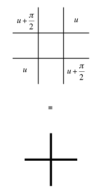
Figure 1: A block of four vertices can be considered as a “supervertex” for a model with $2\times 2=4$ degrees of freedom per edge.

On top of this charge, the antiferromagnetic line exhibits an extra $Z_{2}$ symmetry, as already mentioned in [2]. This can be seen most clearly by considering again the block of spins in Fig. 1 and writing its $\check{R}$ matrix algebraically as (for notations see [2])

$$\check{R}=X_{2}(u)X_{1}(v)X_{3}(v)X_{2}(u),~{}~{}~{}v=u\pm{\pi\over 2}$$ (31)

Using the Yang-Baxter equation repeatedly, one can show that the operator

$$C=X_{1}\left({\pi\over 2}\right)X_{3}\left({\pi\over 2}\right)$$ (32)

commutes with $\check{R}$, where the fact that $X\left({\pi\over 2}\right)=X\left(-{\pi\over 2}\right)$ is crucial. On the other hand, one has [2]

$$X\left(\pm{\pi\over 2}\right)=P_{1}-P_{0}$$ (33)

where $P_{1},P_{0}$ are the projectors on (quantum) spin one and zero representations in the product of two spin $1/2$ representations, so $C^{2}=1$.

We can now discuss briefly the phase diagram of the Potts model in terms of the symmetries of the associated vertex model. The selfdual case $x_{1}={1\over x_{2}}$ gives rise to two kinds of physical behaviors, which correspond in the isotropic case to two selfdual lines, $x_{1}=x_{2}=1$ and $x_{1}=x_{2}=-1$. In the selfdual case, the symmetry of the associated vertex model is $U(1)\times Z_{2}$. The $U(1)$ is just the conservation of the spin $S^{z}$, while the $Z_{2}$ is the symmetry of translation by one lattice site. The latter symmetry, in the continuum limit, becomes another $U(1)$ [19] so the symmetry of the continuum limit on the selfdual lines is $U(1)\times U(1)$: this corresponds to chiral symmetries for left and right fermions, or symmmetry $\phi_{L}\rightarrow\phi_{L}+\alpha$, $\phi_{R}\rightarrow\phi_{R}+\beta$, of the free bosonic continuum limits. Going away from the selfdual lines breaks the $Z_{2}$. If one starts from the physical critical line ($x_{1}=x_{2}=1$), the model becomes massive. If one starts from the non-physical critical line ($x_{1}=x_{2}=-1$), one enters the Berker-Kadanoff phase [2] where the $Z_{2}$ symmetry breaking operator is irrelevant, and the full $U(1)$ is actually restored in the continuum limit.

The antiferromagnetic critical line marks the boundary of the Berker-Kadanoff phase. As just discussed, on this line an extra $U(1)\times Z_{2}$ symmetry appears, and it is reasonable to expect that in the continuum limit, this also gets enhanced into the full $U(1)\times U(1)$, corresponding to another free boson. This is in agreement with the Bethe Ansatz calculation of the central charge. However, when $Q=0$ it has been argued in [18] that this boson is non-compact. This feature must be true along the full antiferromagnetic line in fact, as follows from the finite-size corrections to the gaps.

3.5 The spectrum of the untwisted vertex model for $N$ even

One subtlety is that results for $N$ odd and $N$ even turn out in fact to be profoundly different. We do not understand this fully, but notice this can be expected, as the foregoing analysis applied mostly to $N$ even, which allowed one to treat the two lines $\hbox{Im}\alpha=\pm{\pi\over 2}$. The case of $N$ odd will be considered later. In what follows, we parametrize $\gamma={\pi\over t}$, with $t\in[2,\infty]$.

To start, we consider the XXZ subset some more. Magnetic gaps read

$$\Delta=2\times{g(\tilde{S}^{z})^{2}\over 4}={(\tilde{S}^{z})^{2}\over t}$$ (34)

where $\tilde{S}^{z}$ is the spin of the “equivalent XXZ chain”—that is the chain for which the Bethe equations are (25). Since the antiferromagnetic system has $2N$ spins, whereas the XXZ chain described by (25) is for $N$ spins only, we must rescale the spin according to $\tilde{S}^{z}={S^{z}\over 2}$, where $S^{z}$ is the spin in our initial system, i.e., $S^{z}=\Delta n_{1}+\Delta n_{2}$ in (30). Therefore

$$\Delta={(S^{z})^{2}\over 4t}$$ (35)

where $S^{z}$ (the spin in our initial system) is an integer since we have a even number of spins.

One can see here again why parity effects are likely to occur. If $N$ is even, since we must also have an even number of upturned spins to make up pairs of Bethe roots in the “folding” of the equations, the result strictly speaking will only apply to $S^{z}$ even, including the ground state. Numerical study shows that in fact it holds for $S^{z}$ odd as well. If $N$ is odd on the other hand, since we must also have an even number of upturned spins to make up pairs of Bethe roots in the “folding” of the equations, the result strictly speaking will only apply to $S^{z}$ odd. Numerically, we have observed indeed that for $S^{z}$ even, including the ground state $S^{z}=0$, results for $N$ odd obey a different pattern. See section 7 below.

The electric charges in the $S^{z}=0$ sector of the equivalent XXZ chain are integer ($e=d_{1}=d_{2}$), and give rise to the following gaps $\Delta=2\times{e^{2}\over 4g}={te^{2}\over 4}$. Combining all the excitations, we thus get exponents from a single free boson, $\Delta_{em}={1\over 4}\left({m\over\sqrt{t}}\pm e\sqrt{t}\right)^{2}$, with $e$ and $m$ integers.

Meanwhile, the non-compact boson adds one unit to the central charge, and ‘decorates’ these gaps by soft modes, which would manifest theshelves in a numerical study as very large degeneracies [4]. One can write this in a compact form by considering the generating function of levels

$$Z_{\rm conj}=\sum_{\Delta,\bar{\Delta}}q^{\Delta-c/24}\bar{q}^{\bar{\Delta}-c/24}=\int d\alpha(q\bar{q})^{\alpha^{2}-1/24}\times{1\over\eta\bar{\eta}}\sum_{e,m}q^{\Delta_{em}}\bar{q}^{\bar{\Delta}_{em}}$$ (36)

with $\Delta_{em}(\bar{\Delta}_{em})={1\over 4}\left({m\over\sqrt{t}}\pm e\sqrt{t}\right)^{2}$. It would coincide with the partition function of the doubly periodic vertex model with $q={\rm e}^{-2\pi M/N}$ the modular parameter for a system of size $N\times M$ and $\eta=q^{1/24}\prod_{n=1}^{\infty}(1-q^{n})$ Dedekind’s eta function.

This means that in the sector of vanishing magnetization, one should observe a continuum spetrum above the ground state. In the sector with magnetization unity, one should observe a continuous spectrum over the basic magnetic gap, etc. Numerical study by direct diagonalization of the transfer matrices (possible for $N\leq 12$) is compatible with this result, though the sizes accessible are too small to provide a complete confirmation. In [4] where the Bethe equations themshelves were studied for a simimlar problem, it was found that sizes as large as $N\simeq 10^{4}$ were necessary.

4 The spectrum of the twisted vertex model and the Potts model transfer matrices on the antiferromagnetic line

The usual strategy is, once the continuum limit of the untwisted vertex model is identified, to evaluate the effect of the twisting and other ingredients involved in the correspondence with the loop/cluster formulation, and gain in this way knowledge of the conformal properties of the Potts model itself. The process in the antiferromagnetic region is however more involved than in the ferromagnetic region. To start, we discuss the Berker-Kadanoff phase in more details.

4.1 The Berker-Kadanoff phase

Recall first that the untwisted vertex model in the whole Berker-Kadanoff (BK) phase is described in the continuum limit, like on the non-physical selfdual critical line, by a single free boson with $g={1\over t}$. It is important to notice that this free boson is in fact exactly the same as the one describing the XXZ subset on the antiferromagnetic critical line.

The first step in going from the vertex model to the loop/cluster representation of the Potts model is to introduce a twist in the vertex model. We have explained that this twist has a convenient geometrical interpretation if one decomposes the vertex configurations in loops: without it, loops which are non-contractible around the cylinder get a weight $2$, instead of the required $\sqrt{Q}$ for the loop representation of the Potts model. Suppose we want to give to non-contractible loops a more general weight, $w=2\cos\pi\alpha$. We introduce a seam or twist in the vertex model and the associated conformal weight should give the effective central charge

$$c=1\times\left(1-{6\alpha^{2}\over g}\right)=1-6t\alpha^{2}$$ (37)

Since non-contractible loops come in pairs, we have $\alpha$ defined modulo an integer: these are the allowed values of the electric charge in the Coulomb gas. The $Q$-state Potts model itself corresponds to $\alpha\equiv e_{0}={1\over t}$, leading, in principle, to the central charge $c=1-{6\over t}$.

This latter value is definitely the central charge of the twisted vertex model. But it is not the central charge of the loop/cluster Potts model!

The point is that the eigenvalues of the loop or cluster model are in general (as discussed in section 2) a subset of the eigenvalues of the vertex model, essentially those associated with “highest weights” only. The determination of this subset is based on algebraic considerations, and follows some simple rules [3]. For instance, eigenvalues of the vertex model transfer matrix in the sector of spin $S^{z}=1$ and with no twist are also exactly observed in the sector $S^{z}=0$ and with a twist $\alpha={1\over t}$ (i.e., giving to non-contractible loops the weight $\sqrt{Q}$, that is $\alpha=e_{0}$). Such a “descendent” eigenvalue is thrown away in the loop or cluster formulation.

In the BK phase, the dimension associated with electric charge $e_{0}={1\over t}$, since it is the same as the dimension coming from the sector with no electric charge (twist) and $S^{z}=1$, and equal to $\Delta_{e_{0},0}={1\over 4t}$, is thrown away in the truncation from vertex to loop (or cluster). This means that the central charge of the twisted vertex model and the loop/cluster model are different in this phase. For the vertex model one has $c=1-{6\over t}$ while the central charge of the loop or cluster model follows from the next choice, $e_{0}=1-{1\over t}$, leading instead to central charge $c=1-{6(t-1)^{2}\over t}$, all this for $t$ generic: this is illustrated in Fig. 2.

Figure 2: A schematic representation of the behavior of some levels (in finite size) of the vertex model in the BK phase, for $t$ generic. Levels which are at the head of an arrow are thrown away in going from the vertex to the loop or cluster formulation. The level $\Delta={1\over 4t}$ is thus always discarded, leaving generically the next level $\Delta=(t-1)^{2}/4t$ to determine the central charge $c=1-6(t-1)^{2}/t$ for the loop or cluster model for $t$ generic.

We have performed careful numerical checks of this phenomenon, with some results presented in Figs. 3–4. A technical note here: one can essentially write two transfer matrices, one propagating along the axial direction of the original Potts lattice (and thus diagonally for the medial lattice, which is the lattice where the loops or the vertex spins live), and one propagating diagonally for the Potts lattice (and thus axially for the loops and vertex spins). Results will not (except for parity effects) depend on the geometry in the thermodynamic limit, but might converge better in finite size with one choice or the other. Note that the first formulation is better suited for using the Temperley-Lieb algebra and quantum group symmetries. It is the one we use most. In all figure captions we will use the name diagonal and axial in reference to the medial lattice (see also footnotes 1–2).

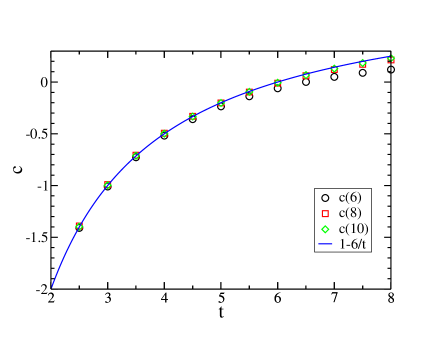
Figure 3: Numerical estimates of the central charge for the twisted vertex model on the non-physical selfdual line. The continuous curve is the expected value, $c=1-6/t$. Diagonal geometry.

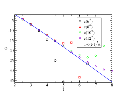
Figure 4: Numerical estimates of the central charge for the loop model on the non-physical selfdual line. The continuous curve is the expected value, $c=1-6(t-1)^{2}/t$. Axial geometry.

Notice that for $t$ an integer (and only then), the eigenvalue associated with $e_{0}=1-{1\over t}$ is also thrown away because it is a descendent from the sector with no twist and spin $S^{z}=t-1$, as illlustrated in Fig. 5. This is the mechanism that, in the periodic case, produces the singularities of the BK phase at the Beraha numbers $Q=4\cos^{2}{\pi\over t}$, with $t$ integer. It is the equivalent of the slightly simpler mechanism studied in [2] in the case of open boundary conditions. In fact, many more levels are thrown away, so many that even the free energy per unit site of the (twisted) vertex and loop or cluster models are different at the Beraha values in the BK phase. The difference of these free energies vanishes as the antiferromagnetic line is approached. Right on the antiferromagnetic line, the free energy does not show any singularity while one crosses a Beraha number (see section 8, in particular Figs. 21–22).

Figure 5: A schematic representation of the behavior of some levels (in finite size) of the vertex model in the BK phase, for $t$ an integer. Now the two levels indicated on the right are both discarded. Many more levels are in fact discarded, leading to the singularities at the Beraha numbers within the BK phase.

A note of caution on the case $t$ integer is in order. Of course, the spectrum of the loop/cluster transfer matrix does not show any particular behavior when one crosses these values. What happens however is that the partition function of the model on a torus, say, would be expressed by weighing these eigenvalues with complicated non-integer ‘degeneracy factors’, and some of these factors can vanish when $t$ is integer, a feature we refer to as a level being truncated, or discarded. Hence what one calls an exponent of the loop/vertex model has to be defined with great care!

4.2 Central charge on the antiferromagnetic critical line

We can now carry out a similar analysis for the model on the antiferromagnetic critical line. To give non-contractible loops a weight $w=2\cos\pi\alpha$, we introduce a seam, and the effective central charge follows immediately as

$$c=2\times\left(1-{6\alpha^{2}\over g}\right)=2-6t\alpha^{2}$$ (38)

since now $g=\frac{2\gamma}{\pi}=\frac{2}{t}$ as in section 3.2. For the $Q$-state Potts model itself we have $\alpha=e_{0}={1\over t}$, leading to a central charge $c=2-{6\over t}$.

Remarkably, this is not only the central charge of the twisted vertex model, but also the central charge of the loop/cluster Potts model on this line, as was established earlier [2], and can be checked numerically to great accuracy. Some results are presented in Figs. 6–7. For Fig. 6 the transfer matrix propagates along the diagonal of the medial lattice, for Fig. 7 along the medial lattice itself. Similar results are obtained for other geometries.

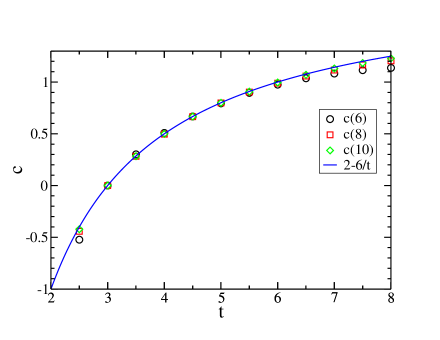
Figure 6: Numerical estimates of the central charge for the twisted vertex model on the antiferromagnetic critical line. The continuous curve is the expected value, $c=2-6/t$. Diagonal geometry.

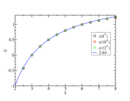
Figure 7: Numerical estimates of the central charge for the loop model on the antiferromagnetic critical line. The continuous curve is the expected value, $c=2-6/t$. Axial geometry.

This result is remarkable, because we have seen that the central charge of the twisted vertex model comes entirely from the XXZ sector, and that this sector is described by the same free boson as in the Berker-Kadanoff phase. Hence one should have expected the level corresponding to (38) to be truncated when going from the vertex to the loop/cluster formulation, and the central charge of the Potts model to be given by another value. What happens is the following.

Observe that the XXZ subset of the spectrum (in the scaling limit) on the antiferromagnetic critical line coincides with the spectrum (in the scaling limit) in the BK phase, with or without twist angle (and up to an additional contribution of one to the central charge). Since, because of the doubling effect discussed previously, the vertex model on the antiferromagnetic critical line has more scaling gaps than in the BK phase, it means that some of the levels which were at finite distance from the ground state in the BK phase have to cross and become scaling levels on the antiferromagnetic critical line. (A similar crossing phenomenon is clearly visible on the finite-size levels of the loop/cluster model, see Fig. 8). One of these levels happens to merge (asymptotically) with the descendent level, so after truncation one of them remains, to give the central charge $c=2-6/t$ still. This is illustrated schematically in Fig. 9.

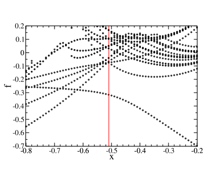
Figure 8: First scaling levels, normalized as free energy densities, of the cluster model with $t=5$ and size $N=6$ (diagonal geometry). The abscissa is the temperature parameter $x=Q^{-1/2}({\rm e}^{K}-1)$. The vertical line shows the bulk antiferromagnetic transition temperature. The ground state on one side of the transition becomes a high excitation on the other side, and vice versa.

Figure 9: The levels corresponding to Fig. 2, but on the antiferromagnetic line. The ground state in the sector $S^{z}=0$, $\alpha={n\over t}$ has now double degeneracy, so that one of the two levels remains after the descendent levels are discarded, leading to the central charge $c=2-{6\over t}$, for any $t$. The additional level comes down from the very excited part of the spectrum as one moves within the BK phase towards the antiferromagnetic critical line.

This is confirmed numerically: we find that the watermelon operator $h_{2}=0$, that is the largest eigenvalue of the loop transfer matrix in the sector with zero legs, and weight $\sqrt{Q}$ for non-contractible loops is asymptotically degenerate with the largest eigenvalue in the sector with two legs, and weight $2$ for non-contractible loops. Since the latter eigenvalue is also observed (as a “descendent eigenvalue”) in the vertex model in the sector with $S^{z}=0$ and twist angle $\alpha=1/t$ (giving to non-contractible loops the weight $\sqrt{Q}$), it follows that the latter sector has a ground state degenerate at least twice. This is the hall mark of a first-order phase transition, and we conclude that the entire antiferromagnetic critical line is in fact a line of first-order critical points for the twisted vertex model. This is also true of the loop model, even though it has fewer eigenvalues, because of the result that $h_{2}=0$. Finally, it is also true for the untwisted vertex model (since its ground state is in fact infinitely degenerate due to the continuous component).

4.3 Spectrum of the loop/cluster model transfer matrix with no marked loops

More generally, the weight $w$ of non-contractible loops is compatible with charges $e=\pm{1\over t}\pm n$, with $n$ an integer. The choice $e=e_{0}-1={1\over t}-1$ leads to a conformal weight (defined over the ground state with $c=2-{6\over t}$)

$$h={(t-1)^{2}-1\over 4t}={t-2\over 4}$$ (39)

This is well observed numerically as seen in Fig. 10. We believe that there is a continuum spectrum on top of this gap, all of which is truncated when one goes from the Potts transfer matrix to the Potts partition function when $t$ is integer.

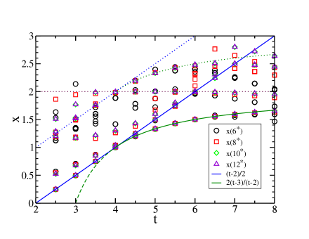
Figure 10: Spectrum of the loop/cluster Potts model transfer matrix in the sector with no marked loops/clusters. Two exponents are clearly identified (solid lines) as well as descendent levels (dotted lines). Axial geometry.

One can also identify numerically a level very well matched by the formula $h={t-3\over t-2}$. This has no natural explanation within the XXZ subset, and will be discussed in details below.

We will argue later that the spectrum is in fact continuous above $h={t-2\over 2}$. This is all for $t$ generic of course. For Beraha numbers, the continuous component disappears entirely, as well as other exponents.

4.4 Spectrum of the twisted vertex model transfer matrix in the sector $S^{z}=0$

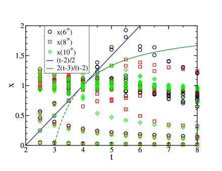
Figure 11: Spectrum of twisted vertex model transfer matrix in the sector $S^{z}=0$. Axial geometry. Note the considerable set of additional levels when compared to Fig. 10. The particular levels identified with solid lines in Fig. 10 are also present here.

Exponents are shown in Fig. 11. Observe how one sees considerably more levels than in the loop/cluster model case (see Fig. 10). We will argue later that here, the spectrum is in fact continuous above the ground state $h=0$.

4.5 Watermelon operators

These operators describe the properties of $L$ marked lines in the loop model (or, for even $L>2$, equivalently by $L/2$ marked clusters in the cluster model). As usual, their conformal weight is obtained by considering the ground state of the sector with $S^{z}={L\over 2}$ ($L$ even), so, with respect to the ground state of the theory with central charge $c=2-{6\over t}$, we find

$$h_{L}={(L/2)^{2}-1\over 4t}$$ (40)

This is also well checked numerically, as can be seen in Fig. 12.

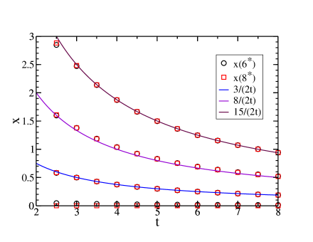
Figure 12: Watermelon exponents on the antiferromagnetic critical line, in the loop model with $L=2,4,6,8$ marked lines. Axial geometry.

Notice in particular that the case $L=2$ corresponds to $h_{2}=0$.

5 RSOS versions at the Beraha numbers

As commented earlier, the Potts model does present singular behaviour at the Beraha numbers in the Berker-Kadanoff phase because the largest eigenvalues of the loop transfer matrix do not contribute to the partition function. Eigenvalues which actually do contribute are related, though not identical, to those of another version of the model, of the restricted solid-on-solid (RSOS) type. These RSOS models are particularly interesting to study as they are completely local models of statistical mechanics, and thus should correspond to well defined conformal field theories, presumably “minimal” with respect to some chiral algebra, and hence easier to identify.

RSOS models can be defined whenever $t$ (in $q={\rm e}^{i\pi/t}$) is rational, $t=r/s$. Their variables are integer heights $h_{i}=1,2,\ldots,r-1$ living on the union of direct and dual lattice sites (i.e., again a diagonally oriented square lattice, but shifted with respect to the medial lattice), subject to the RSOS constraint $|h_{i}-h_{j}|=1$ for neighboring $i$ and $j$. The Boltzmann weights are most easily defined by writing the row-to-row transfer matrix [20, 2]

$$T=Q^{N/2}\prod_{i=1}^{N}\left(\frac{{\rm e}^{K}-1}{Q^{1/2}}+e_{2i-1}\right)\prod_{i=1}^{N}\left(1+\frac{{\rm e}^{K}-1}{Q^{1/2}}\,e_{2i}\right)$$ (41)

in terms of Temperley-Lieb generators $e_{j}$. The latter are represented as

$$(e_{j})_{h,h^{\prime}}=\delta(h_{j-1},h_{j+1})\,\prod_{i\neq j}\delta(h_{i},h^{\prime}_{i})\,\frac{(S_{h_{i}}S_{h^{\prime}_{i}})^{1/2}}{S_{h_{i-1}}},$$ (42)

where $S_{h}=\sin(\pi hs/r)$.

In the transfer matrix study of the RSOS models, the basis states are collections of $2N$ heights $h_{1},h_{1},\ldots,h_{2N}$ belonging alternately to the direct and dual lattice, and subject to the constraint $|h_{i}-h_{i+1}|=1$. To have periodic boundary conditions in the $x$-direction we impose $h_{2N+i}=h_{i}$. One can show that ${\rm dim}\ T\simeq\left[2\cos(\pi/r)\right]^{2N}=Q^{N}$ when $N\gg 1$.

Of course, the correspondence between the partition function of the RSOS model, the partition function of the Potts model, and the spectrum of the loop/cluster transfer matrix or twisted vertex model transfer matrix is rich and intricate. For instance, the partition function of the RSOS model with doubly periodic boundary conditions on a torus would read [20]

$$Z=Q^{S/2}\sum_{E\subseteq\langle ij\rangle}Q^{[l(E)-l_{0}(E)]/2}\left({{\rm e}^{K}-1\over Q^{1/2}}\right)^{|E|}\ \sum_{a=1}^{r-1}\left(2\cos{\pi a\over r}\right)^{l_{0}(E)}$$ (43)

where the number of non-contractible loops $l_{0}(E)$ has been singled out. This formula indicates that, in the vertex model, $r-1$ sectors with different values of the twist are now necessary.

In this paper we shall restrict the study to $t$ integer (i.e., $r=t$ and $s=1$), and use the identification of the associated conformal field theory to strenghten our general results (on the critical ferromagnetic line for instance, the CFT for the RSOS models would be the minimal theory with central charge $c=1-6/t(t-1)$).

The critical antiferromagnetic variety does not intersect the selfdual manifold, and thus corresponds to a staggered RSOS model. We are not aware of any previous study of such model.

To proceed, let us define the four regimes

$$0 <u< \gamma~{}~{}(i)$$

$$\gamma <u< {\pi\over 2}~{}~{}(ii)$$

$${\pi\over 2} <u< \gamma+{\pi\over 2}~{}~{}(iii)$$

$$\gamma+{\pi\over 2} <u< \pi~{}~{}(iv)$$ (44)

The Potts model on the antiferromagnetic critical line involves two kinds of vertices, with spectral parameters differing by ${\pi\over 2}$. Hence, either they lie in regimes $(i),(iii)$ or in regimes $(ii),(iv)$.

We can go from the Potts model to the RSOS model algebraically by using a different representation of the Temperley-Lieb algebra (that is, ‘quantum group restricting’ the vertex model representation). A homogeneous spectral parameter $u$ (such as would be obtained on the selfdual lines) would lead to a homogeneous RSOS model of the type studied by Andrews, Baxter and Forrester [21]. To dispel confusion, we will reserve the name ABF to homogeneous models, and denote the restricted version of the vertex model on the antiferromagnetic line (as well as elsewhere in the phase diagram) as the RSOS model (in general, staggered). Where, in the ABF phase diagram, these models stand is an interesting question. For $u$ in regimes $(i)$ or $(iii)$, the ABF model is at the transition point between its regime $III$ and regime $IV$ (capital letters refer to the regimes originally defined in [21]), while for $u$ in regimes $(ii),(iv)$, the ABF model stands at the transition point between its regime $I$ and regime $II$. Based on this observation, we see that we ought to expect that the antiferromagnetic Potts model, for a given value of $Q$, can be in two different universality classes, depending on the anisotropy. The isotropic case is what we are interested in here: $K_{1}=K_{2}$ corresponds to the SDP (self-dual Potts) models in regimes $(ii),(iv)$ and thus the ABF models at the transition between regime $I$ and $II$. In fact, only the regime $(ii)$ corresponds to a physical ABF model, and thus was studied in [21].

Now remarkably, the central charge we have found for the isotropic Potts model on the antiferromagnetic critical line coincides with the one of the associated ABF model at the transition between regime $I$ and regime $II$ for $t$ an integer, $t\equiv k+2$. It is therefore tempting to conjecture that the RSOS version of the antiferromagnetic critical line for $k=t-2$ an integer is in the universality class of the ABF models at the transition between regime I and regime II, and thus, following [21, 22] is a theory of $Z_{k}$ parafermions. Let us discuss further the evidence for this.

An immediate objection to this claim might be that the ABF models are not at a first-order critical point. Indeed, they are not, and the point is that when one goes from the twisted vertex model to the RSOS models, the eigenvalues from the untwisted $S^{z}=1$ sector are discarded ($L=2$ watermelon), as well as the descendent eigenvalues in the $S^{z}=0$ sector with twist $\alpha={1\over t}$. Therefore, the second $h=h_{2}=0$ exponent disappears, and there is no reason to expect a first-order phase transition any longer. This is illustrated in Fig. 13.

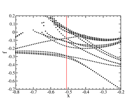
Figure 13: Same as Fig. 8 but for the RSOS model. Remark the absence of levels responsible for the BK phase. Some levels are identical with those of the cluster model, including the ground state on the high-$x$ side of the transition. This ground state does not participate any level crossings.

Note that in the ABF language, the extra $Z_{2}$ symmetry which appears on the antiferromagnetic critical line corresponds to the chiral symmetry of the $Z_{k}$ models discussed in [22], that exchanges clockwise and counterclockwise.

The ABF models at the transition between regime $I$ and regime $II$ have parafermionic exponents, of the general form [23]

$$h={l(l+2)\over 4(k+2)}-{m^{2}\over 4k},\quad l=0,1,\ldots,k;\quad-l\leq m\leq l;\quad l-m=0\hbox{ mod }2$$ (45)

and

$$h={(k-l)(k-l+2)\over 4(k+2)}-{(k-m)^{2}\over 4k},\quad l=0,1,\ldots,k;\quad l\leq m\leq 2k-l-2;\quad l-m=0\hbox{ mod }2$$ (46)

All these exponents (and only these) are indeed observed numerically in the RSOS model on the antiferromagnetic critical line: see Fig. 14.

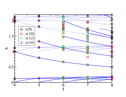
Figure 14: Exponents for the RSOS model on the antiferromagnetic critical line, and comparison with the spectrum of the $Z_{k}$ model. Solid lines show the exponents (45), while dashed lines represent descendents. Diagonal geometry.

On the other hand, by the quantum group construction [3], the eigenvalues of the RSOS models are obtained by combining sectors of the vertex model with vanishing spin and twists $\alpha={(l+1)\over(k+2)}$ (recall, $t\equiv k+2$), $l$ integer, $0\leq l\leq k$. The associated dimension in the XXZ part of the spectrum is obtained by setting $e={l+1\over k+2}$, and coincides with the one from the sector with vanishing twist and $S^{z}=l+1$; as such, this eigenvalue disappears from the loop model in the BK case. On the antiferromagnetic line however, this value is still observed: like in the case $l=0$, there is double degeneracy in the vertex model, so the loop model still has this exponent. Observe now that this exponent (with respect to $c=2-\frac{6}{t}$) agrees with formula (45) for the same $l$ and $m=0$.

For a given $l$, the parafermionic tower gives weights (45). We recognize there the value coming from the XXZ subset, from which the quantity ${m^{2}\over 4k}$ has been subtracted. In particular, in the sector with twist $\alpha=\frac{l+1}{k+2}$, the lowest lying excitation should not be given by $m=0$ (unless $l=0$) but by the dimension of the order parameter in the $Z_{k}$ theory, which corresponds to $l=m$ and reads

$$h_{l}={l(k-l)\over 2k(k+2)}$$ (47)

Replacing by the value of $\alpha$ gives the result

$$h_{\alpha}={((k+2)\alpha-1)(k+1-(k+2)\alpha)\over 2k(k+2)}$$ (48)

The simplest way to put these results together is that the spectrum should contain, for any value of $\alpha$, the XXZ value (with respect to the ground state with $c=2-{6\over t}$) $h={[(k+2)\alpha]^{2}-1\over 4(k+2)}$. But on top of this, it should also contain other eigenvalues which have double degeneracy, (48) being the lowest one for $\alpha={l+1\over k+2}$. Only for $l=0$, i.e., $\alpha={1\over k+2}$ will the two coincide. This pattern should presumably extend to $t$ generic.

Numerical study for the leading exponent in the sector of twist $\alpha$ as a function of $\alpha$ is illustrated in Fig. 15. One sees that for $|\alpha|<{1\over t}$, the XXZ formula holds, while beyond this, it has to be replaced by the formula (48) with $t\equiv k+2$, and $t$ now arbitrary, as expected.

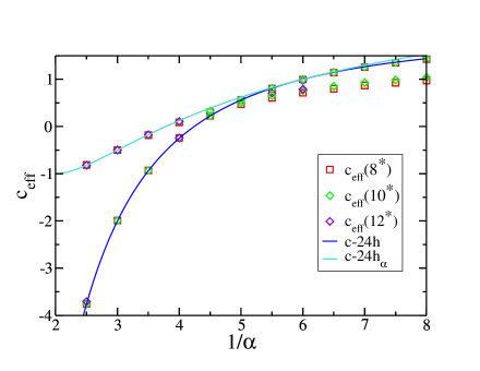
Figure 15: Effective central charge for $t=6$ in the sector with $S^{z}=0$ and twist $\alpha$. For $\alpha\leq{1\over t}$, the XXZ gap determines the effective central charge $c_{\rm eff}=c-24h=2-6t\alpha^{2}$ (blue line), while beyond this value, the effective central charge is determined by a different gap, whose origin will be related to a non-compact boson later, $c_{\rm eff}=c-24h_{\alpha}=-1+{3t\over t-2}(2\alpha-1)^{2}$ (cyan line). Axial geometry.

Exponents with $-l\leq m\leq l$ should also be present, but we have had difficulties identifying them numerically in general. An exponent which we have identified however corresponds to (46) with $l=0$ and $m=2$: it is the exponent of the first (most relevant) parafermionic chiral current, with

$$h={k-1\over k}$$ (49)

While we have argued that the spectrum has a continuous component for the vertex model and the loop/cluster model, there is of course no such component in $Z_{k}$ models, and therefore all the corresponding exponents must disappear in the RSOS partition function. This is in particular the case for the continuous branch in the sector $l=0$, which starts at $h={t-2\over t}={k\over k+2}$.

6 A free field representation for the antiferromagnetic Potts model

To put all these elements together in the construction of a fully consistent conformal field theory for the cluster/loop Potts model does not seem straightforward, and is plagued with the usual difficulties, in particular logarithmic features—such a fully consistent construction is not available even in the much simpler case of the ferromagnetic critical line. Like in the latter case, some progress can be made however by using a free field representation.

This free field representation is inspired by two features. First, we have deduced the presence of a compact boson and a non-compact boson from the Bethe ansatz analysis. Second, the value of the central charge at the Beraha numbers $t=k+2$ coincides (as was observed in [2]) with the central charge for $Z_{k}$ models, and for the latter, a free field representation based on a pair of bosons, one compact and one non-compact, is well known [24] (see also [25, 26]).

We thus start, following [24] by introducing a pair of bosonic fields $\phi_{1}$ and $\phi_{2}$, with propagators

$$\langle\phi_{1}(z)\phi_{1}(w)\rangle = -2\ln(z-w)$$

$$\langle\phi_{2}(z)\phi_{2}(w)\rangle = -2\ln(z-w)$$

and a stress tensor

$$T=-{1\over 4}\left(\partial\phi_{1}\right)^{2}+{1\over 4}\left(\partial\phi_{2}\right)^{2}+i\alpha_{0}\partial^{2}\phi_{1}$$ (51)

With a charge at infinity $\alpha_{0}={1\over 2\sqrt{t}}$ for the first boson $\phi_{1}$, the central charge is $c=2-{6\over t}$.

There are various ways to introduce screening operators in this theory. The first choice, which was used in [24] uses both bosons $\phi_{1},\phi_{2}$, and leads to the three currents

$$J_{1}=\partial\phi_{2}\exp\left[2i\alpha_{0}\phi_{1}\right]$$ (52)

together with

$$J_{\pm}=\exp\left[-{i\over 2}\sqrt{t}\phi_{1}\pm{1\over 2}\sqrt{t-2}\phi_{2}\right]$$ (53)

These screening operators, having conformal dimension one, commute with the Virasoro algebra. It turns out that they also commute with the “parafermionic” currents

$$\Psi=-{i\over 2}\left(\sqrt{t\over t-2}\partial\phi_{1}+i\partial\phi_{2}\right)\exp\left[{1\over\sqrt{t-2}}\phi_{2}\right]$$

$$\Psi^{\dagger}=-{i\over 2}\left(\sqrt{t\over t-2}\partial\phi_{1}-i\partial\phi_{2}\right)\exp\left[-{1\over\sqrt{t-2}}\phi_{2}\right]$$ (54)

The vertex operators

$$V_{lm}=\exp\left[-i{l\over 2\sqrt{t}}\phi_{1}+{m\over 2\sqrt{t-2}}\phi_{2}\right]$$ (55)

then play a special role: the action of $J_{\pm}$ on $V_{lm}$ is only well defined for $l$ integer and $l\pm m$ even. $V_{lm}$ is annihilated by the corresponding charges $Q_{\pm}$ iff $-l\leq m\leq l$. Similarly, if we consider the action of powers of $Q_{1}$, it is well defined only in the case $Q_{1}^{l+1}$ acting on $V_{lm}$, unless $t$ is rational—we will suppose it is not the case here. Then $Q_{1}^{l+1}V_{lm}=0$. Finally, one can get outside the range $-l\leq m\leq l$ by acting with the parafermionic fields, which are also annihilated by $Q_{\pm}$ and $Q_{1}$.

The case $l=0$ leaves fields obtained by successive action of the parafermionic fields on the identity, the lowest of which has dimension $h={t-3\over t-2}$ and is twice degenerate.

We call the fields obtained in this way the first Coulomb gas contribution. In this sector, $\phi_{2}$ presumably does not contribute a continuous part, as the corresponding charges are constrained by the screening operators.

Note that we can also consider twisting differently the boson $\phi_{1}$ with $\tilde{\alpha}_{0}={t-1\over 2\sqrt{t}}$. Introducing the usual screening charges for a one boson theory, $\alpha_{+}\alpha_{-}=-1$, $\alpha_{+}+\alpha_{-}=2\tilde{\alpha}_{0}$, the corresponding screening currents read

$$\tilde{J}_{\pm}=\exp\left[i\alpha_{\pm}\phi_{1}\right]$$ (56)

The usual Felder construction [27] gives the allowed vertex operators

$$\Phi_{rs}=\exp\left[\left(i\,{1-r\over 2}\,\alpha_{+}+i\,{1-s\over 2}\,\alpha_{-}\right)\phi_{1}\right]$$ (57)

The central charge and the dimensions are not those expected; $c=2-6{(t-1)^{2}\over t}$ (the additional contribution of one coming from the boson $\phi_{2}$) and $h={(tr-s)^{2}-(t-1)^{2}\over 4t}$. But this theory is non-unitary, and admits in particular the negative-dimension operator with $r=0,s=1$, leading to an effective central charge $c=2-{6\over t}$ which coincides with the central charge of the loop/cluster Potts model. The exponents with respect to this effective central charge are

$$h={(tr-s)^{2}-1\over 4t}$$ (58)

and in particular, the choice $r=s=1$ gives the gap $h={t-2\over t}$. The $L$-leg operators correspond meanwhile to $h_{0,L/2}$ ($L$ even in the Potts model).

In this sector, $\phi_{2}$ is not constrained, and presumably contributes a continuous spectrum, starting therefore right at the effective central charge.

The “full Coulomb gas” is expected to describe the twisted vertex model: in particular, the degeneracy two of the effective ground state with $c=2-{6\over t}$ is reproduced in our picture. Some of the levels of the twisted vertex model were represented earlier.

Going to the loop/cluster Potts model involves discarding some levels, such as the $r=0$, $s=1$ field above. The continuum then should only start at the true central charge, i.e., the gap $h={t-2\over t}$ with respect to $c=2-{6\over t}$.

When $t$ is rational, going to the RSOS model involves discarding many more levels, and restricting these Coulomb gases to minimal conformal field theories. In the special case $t=k+2$ an integer, the corresponding minimal model for the second Coulomb gas is $M_{k+2,1}\times$ [non-compact boson $\phi_{2}$] and is actually empty. This leaves only the first Coulomb gas, whose restriction gives the $Z_{k}$ parafermionic theory. This agrees in particular with our prediction that the continuous component should disappear at $t=k+2$ an integer. The case $t$ rational meanwhile should retain some of the continuous component.

7 The case $N$ odd

Numerical study shows that the ground state in the sector with $N$ odd does not scale like the ground state for $N$ even. Maybe the best way to understand this is to start by discussing the untwisted vertex model, and the associated watermelon operators. We find that the ground state of the untwisted vertex model exhibits an effective central charge

$$c_{\rm eff}={1\over 2}$$ (59)

independently ot the value of $t$, as illustrated in Fig. (16). This is in contrast with the value of $c=2$ we found earlier for the case $N$ even.

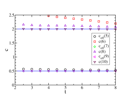
Figure 16: The central charge of the untwisted vertex model on the antiferromagnetic critical line for $N$ odd takes the value $c_{\rm eff}={1\over 2}$ in contrast with the value $c_{\rm eff}=2$ for $N$ even. Diagonal geometry.

The simplest interpretation of this result is that the odd parity acts as a disorder line, corresponding to a disorder operator with dimension $\Delta={1\over 16}$. This in turn can be interpreted within the Coulomb gas by assuming that one of the two bosons sees antiperiodic boundary conditions in the space direction. The determination of the watermelon exponents (see below) gives the values

$$h_{L}={(L/2)^{2}-1\over 4t}+{1\over 16}$$ (60)

showing that the contribution from the boson $\phi_{1}$ is as in the $N$ even case, and thus it must be the non-compact boson $\phi_{2}$ that is twisted, i.e., sees antiperiodic boundary conditions.

Notice that if the field $\phi_{2}$ is twisted in the $N$ odd sector, the continuous part of the spectrum must disappear, as the twisted sector of a compact and non-compact bosons are identical. The spectrum for $N$ odd thus ought to be considerably simpler than for $N$ even, a fact well in agreement with numerical studies.

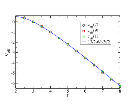
Figure 17: Effective central charge for the loop model on the antiferromagnetic critical line in the sector $N$ odd (diagonal geometry). The solid line shows the expected result, $c_{\rm eff}=c-24h_{D}=\left(2-\frac{6}{t}\right)-24\left(\frac{t-3}{16}\right)$.

We now turn to the loop/cluster Potts model. The effective central charge is found numerically (see Fig. 17) to be given by a field of dimension

$$h_{D}={t-3\over 16}$$ (61)

To interpret the presence of the weight (61) in general, we observe that it can be written

$$h_{D_{0}}={1\over 16}+{t\over 4}\left({1\over 2}-{1\over t}\right)^{2}-{1\over 4t}$$ (62)

As argued earlier, the ${1\over 16}$ contribution comes from an antiperiodic sector for the non-compact boson $\phi_{2}$. The remaining contribution can then be interpreted as the weight for an electric charge $\tilde{e}_{0}={1\over 2}-{1\over t}$ in the $\phi_{1}$ theory. Recall that in the $N$ even sector we had charges $e_{0}={1\over t},1-{1\over t},\ldots$ instead. We do not know the origin of this additional ${1\over 2}$ contribution to the charge.

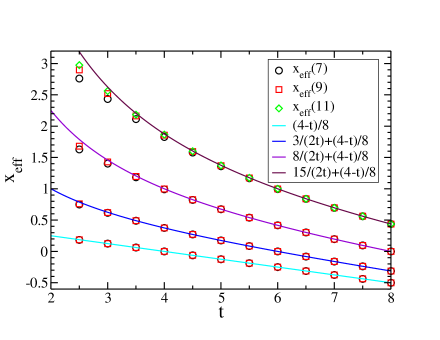
Figure 18: Effective watermelon exponents, in the sector $N$ odd, for the loop model along the antiferromagnetic critical line. Diagonal geometry.

Effective watermelon exponents in the twisted vertex model (and in the loop model) are then given by measuring the gaps with respect to the odd-$N$ ground state. This yields

$$h_{L}^{\rm eff}=h_{L}-h_{D_{0}}={(L/2)^{2}-1\over 4t}+{4-t\over 16}$$ (63)

and is verified numerically in Fig. 18.

For $t=k+2$ an integer, the above results can be fitted in a parafermionic picture by introducing the disorder operators (with respect to charge conjugation symmetry), whose weights read [28]

$$h_{D_{s}}={\left[k-2+(k-2s)^{2}\right]\over 16(k+2)},\qquad 0\leq s\leq{k\over 2}$$ (64)

The largest of these weights is obtained for $s=0$, and coincides with (61). On the other hand, it is well-known that correlation functions in the disorder sectors have to be defined on a two-sheet Riemann sphere, implying in particular the presence of descendents on half-integer levels. We expect this feature to extend to $t$ generic, and this is indeed well verified by the numerics for the first excitations in the odd-$N$ sector, both for the loop model and for the twisted vertex model. We spare the reader the corresponding figures.

8 Other exponents of the antiferromagnetic Potts model

We consider first the magnetic exponent. In the Berker-Kadanoff phase, it is obtained by putting an electric charge at infinity so as to cancel the weight of non-contractible loops ($\alpha={1\over 2}$), and

$$h_{H}^{\rm BK}={t\over 16}-{(t-1)^{2}\over 4t}.$$ (65)

The dimension in the untwisted boson theory is thus $\Delta_{H}^{\rm BK}={t\over 16}$. The dimension on the antiferromagnetic line, conjectured first in [2], is obtained by adding a contribution from the non-compact boson, so

$$h_{H}^{\rm AF}={t\over 16}-{1\over 4t}-{t-2\over 16}={1\over 8}-{1\over 4t}.$$ (66)

This value is easy to understand following the discussion after formula (48): the magnetic exponent corresponds indeed to $\alpha={1\over 2}$ (a value which kills non-contractible loops, in relation with the term having $\eta(E)=1$ in (3)), for which the XXZ value is never valid as $t\geq 2$ always, while the correct value deduced from the parafermionic exponents gives $c_{\rm eff}=-1$, in agreement with the conjectured value of $h_{H}^{\rm AF}$.

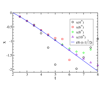
Figure 19: Magnetic exponent of the loop model along the non-physical selfdual line. Axial geometry. The solid line represents the result (65).

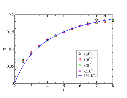
Figure 20: Magnetic exponent of the loop model along the critical antiferromagnetic line. Axial geometry. The solid line represents the result (66).

The results (65)–(66) for the magnetic exponent are verified numerically in Figs. 19–20.

Next, we consider the thermal exponent. An increase of $K$ moves the model into a massive phase, while a decrease moves it into the Berker-Kadanoff (BK) phase. Numerical evidence is that the BK and massive phases are not related analytically in any way, and that the largest eigenvalue in the masive phase becomes the smallest (or maybe one of the smallest, in the sense that it scales with the smallest) eigenvalue in the BK phase. As a result, the free energy per unit area for the Potts model at $Q$ generic and the twisted vertex model exhibits a discontinuity of the first derivative at the antiferromagnetic critical point, a characteristic of first-order phase transitions. Nevertheless, we have amply argued that these models right at the critical point have algebraic decaying correlations. We are thus in a case of a first-order critical point with an exponent $\nu=1/2$ all along the line for the twisted vertex model, and, generically, for the loop/cluster Potts model.

On the other hand, these results do not apply to the loop/cluster Potts model in the case of $Q$ a Beraha number, that is $t=k+2$ integer. For such values of $Q$, the free energy does not exhibit a kink any longer, the eigenvalues crossing the ground state at the antiferromagnetic critical point being cut-off from the partition function within the Berker-Kadanoff phase. The same is true for the RSOS version of the model. These different features are illustrated in Fig. 21.

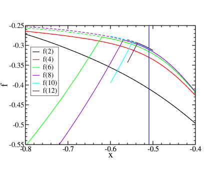
Figure 21: The dashed (resp. solid) curves represent the free energy of the RSOS model (resp. the loop model) at $t=5$ for various widths $N$. The two free energies coincide perfectly (and hence, also with that of the twisted vertex model) for $x=Q^{-1/2}({\rm e}^{K}-1)$ large enough (whence the dashed curves are ‘hidden’ by the solid ones). However, for smaller $x$, the free energy of the loop model experiences a sharp singularity with a discontinuity of the derivative. As $N$ increases, this singularity moves towards the bulk antiferromagnetic transition temperature, here shown as a vertical line. Within the BK phase, the free energies of the RSOS and the loop models are different, with a jump whose magnitude increases as one goes deeper within this phase. Diagonal geometry.

While the existence of the first-order critical point can be pretty much argued analytically for the twisted vertex model and the Potts model, it is natural to expect a similar transition in the untwisted vertex model, since for the vertex model, the free energy per unit area should behave “normally” and thus be independent of twists. This is confirmed by numerical study, as illustrated in Fig. 22.

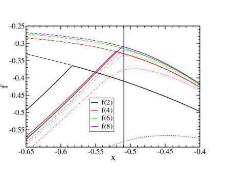
Figure 22: The dotted (resp. full) curves represent the free energy of the untwisted (resp. the twisted) vertex model at $t=5$ for various widths $N$. The dashed curves are for the RSOS model, same as in Fig. 21. Only the twisted vertex model exhibits singular behavior for finite $N$. However, the free energies of the twisted and untwisted vertex model behave similarly in the thermodynamic limit, with a first-order critical point on the antiferromagnetic critical line. Diagonal geometry.

At the Beraha numbers, and for the loop/cluster Potts model or the RSOS model, the thermal operator does not have dimension ${1\over 2}$ any more. Rather, the dimension becomes $h={k-1\over k}={t-3\over t-2}$, the dimension of the parafermion operator. It is easiest to find out what happens for the RSOS version of the model, which has the same largest eigenvalue as the loop/cluster model. In this case, recall that the antiferromagnetic critical point is in the universality class of the $Z_{k}$ theory, and the flow in the Berker-Kadanoff phase coincides with the flow predicted by Fateev and Zamolodchikov [29] who studied perturbed parafermionic theories with the following hamiltonian:

$$H=H_{k}+\lambda\left({\rm e}^{i\theta/k}\psi\bar{\psi}+{\rm e}^{-i\theta/k}\psi^{\dagger}\bar{\psi}^{\dagger}\right)$$ (67)

($\lambda$ positive by convention). These authors argued that for $\theta=\pi$ the theory flows, for $k$ odd, to the minimal model with central charge $c=1-{6\over(k+1)(k+2)}$ while it remains massive for $k$ even.

Numerical evidence for these flows is presented in Figs. 23–25, where we also give phenomenological interpretations of other relevant features in the RSOS model phase diagrams.

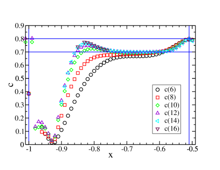
Figure 23: Parafermion to minimal model flow in the RSOS model with $t=5$. The parameter $x=Q^{-1/2}({\rm e}^{K}-1)$. The vertical lines show the non-physical selfdual line ($x=-1$) and the antiferromagnetic critical point ($x\simeq-0.51$). The horizontal lines are at $c=4/5$ and $c=7/10$, the central charges of the relevant parafermion and minimal models. The data indicates the existence of a new repulsive fixed point at $x\simeq-0.83$ in the parafermion model universality class. The minimal model fixed point is situated somewhere between this and the antiferromagnetic point, and its attractive nature leads to a plateau in $c$ in the range $-0.83<x<-0.51$. The data further reveal a $c=0$ fixed point, presumably repulsive, at $x\simeq-0.93$. If true, consistency of the RG flow diagram would necessitate another attractive fixed point; the data is indeed consistent with such a point at $x\simeq-0.87$, again in the minimal model universality class. The interpretation of the data in the range $-1<x<-0.93$ is somewhat uncertain. Right at $x=-1$, the data are again well-behaved and converge to $c=-0.385\pm 0.001$. We have no explanation for this value at present. Diagonal geometry.

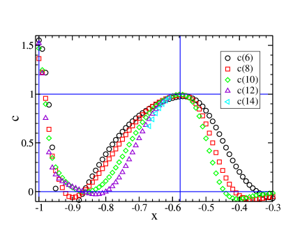
Figure 24: RSOS model phase diagram for $t=6$. The physics is different—and simpler—than in the case $t=5$ shown in Fig. 23. The $c=1$ parafermion fixed point at the antiferromagnetic transition, $x\simeq-0.58$, is still repulsive, but the nearest attractive fixed point is now the non-critical $c=0$ point at $x\simeq-0.87$. Right at $x=-1$ the data converge slowly towards $c=1.6\pm 0.1$, an unexplained value. The model is expected to be massive everywhere, except at the two vertical lines. Diagonal geometry.

Figure 25: RSOS model phase diagram for $t=7$. The physics is similar to the case of $t=5$ shown in Fig. 23. In particular, we observe again a parafermion ($c=\frac{8}{7}$) to minimal model ($c=\frac{6}{7}$) flow. The plateau at $c=\frac{6}{7}$ develops more slowly in $N$, in the form of a ‘shoulder’. Analyzing the behavior at the left edge of that plateau would call for larger system sizes than those presented here. Diagonal geometry.

Note meanwhile that if $t$ is rational, we can still define an RSOS model, but its ground state energy should be the same as the one of the vertex model—that is, exhibit the first-order critical point, in sharp contrast with what happens for $t$ integer. This is illustrated in Fig. 26 for $t={5\over 2}$.

Figure 26: The free energy of the RSOS model for $t={5\over 2}$ also develops a first-order singularity in the thermodynamic limit. Diagonal geometry.

Finally the question remains of how to describe the first-order critical point within the Coulomb gas. We have not found the complete answer to this question, but a probable scenario is that we are dealing with the perturbation described by Fateev [30],

$$H=H_{0}+\Lambda\cos(\beta_{1}\Phi_{1})\cosh(\beta_{2}\Phi_{2})$$ (68)

where $H_{0}$ is the hamiltonian for a pair of free bosons $\Phi_{1}$ and $\Phi_{2}$ as in section 6, and

$$\beta_{1}^{2}-\beta_{2}^{2}=4\pi$$ (69)

Indeed, consider first the case where the boson $\Phi_{1}$ is twisted so that the central charge is $c=2-{6\over t}$, and set ${\beta_{1}^{2}\over 8\pi}={t\over 4}$. By standard Coulomb gas calculations one finds then the dimension of the perturbation to be $h={\beta_{1}^{2}-\beta_{2}^{2}\over 8\pi}\pm{1\over 2}=0,1$, i.e., a mix of a perturbation with dimension zero and one with dimension unity. Meanwhile, the theory is integrable, and admits non-local conserved currents, one of them being

$$J_{\pm}=\partial\phi_{1}\exp\left(\pm{4i\pi\over\beta_{2}}\phi_{2}\right)$$ (70)

with dimension $h=1-{2\pi\over\beta_{2}^{2}}=1-{1\over t-2}={t-3\over t-2}$, the dimension of the parafermionic current. [The other current meanwhile is

$$J^{\prime}_{\pm}=\partial\phi_{2}\exp\left(\pm{4i\pi\over\beta_{2}}\phi_{1}\right)$$ (71)

with dimensions $h=1$ and $h={t+2\over t}$.] A priori, the integrable perturbation involves a mixture of all these operators. What must happen is that for $t$ integer, the quantum group truncation leaves only the contribution from $J_{\pm}$, leading to the parafermionic perturbation. Otherwise, the two relevant operators have dimension zero and ${t-3\over t-2}$, presumably in agreement with our observation of a first-order critical point for the generic Potts model.

Now in the untwisted theory, the perturbation in (68) has dimension $h={1\over 2}$, the one of $J_{\pm}$ is as before, and the one of $J^{\prime}_{\pm}$ is $h={t+1\over t}$. One might be concerned by the absence of a dimension zero operator then, since we have argued that the untwisted vertex model had a first-order critical point as well. The point is that the coupling constant $\Lambda$ in (68) must be identified with the lattice coupling $K-K_{\rm c}$ within the twisted theory, as multiplying the field of dimension zero in the twisted theory. Let us call it $\Lambda_{\rm tw}$ for clarity. Then the physical dimension of $\Lambda_{\rm tw}$ is $[L]^{-2}$. In the untwisted theory, the perturbation has physical dimension $[L]^{-2h}=[L]^{-1}$, so the coupling there must also have dimension $[L]^{-1}$, i.e., be proportional to the square root of $\Lambda_{\rm tw}$, or the square root of $K-K_{\rm c}$. A singularity of the free energy such as $|K-K_{\rm c}|$ turns into $|\Lambda_{\rm tw}|$ i.e., $\Lambda_{\rm untw}^{2}$ from dimensional counting, corresponding, within the untwisted theory, presumably to $\Lambda_{\rm untw}|\Lambda_{\rm untw}|$, i.e., a thermal exponent $\alpha=0$, and thus an exponent $\nu={1\over 2}$, a perturbation of dimension $h={1\over 2}$ indeed.

Making this more precise is left for future work: it seems clear in any case that the variable $K$ is not very natural to study the perturbations of the untwisted theory.

A last observation we can make is that, since the parafermionic theories for $t$ integer flow to minimal theories in the BK phase, and since the latter are derived from a Coulomb gas with coupling $g={t-1\over t}$, it is most likely that excitations for $Q$ generic around the “false ground state”—i.e., the state that crosses from the higk $K$ phase, and that would still be the ground state of the Potts model for $Q$ a Beraha number—are described by this Coulomb gas, at least in the vicinity of the antiferromagnetic transition. Excitations around the true ground state meanwhile are described by a Coulomb gas with $g={1\over t}$, so both manifolds are in fact present within the BK phase!

9 Conclusion

The least one can say is that the properties of the antiferromagnetic Potts model are extremely complex, even for the simple case of the square lattice. There are definitely loose ends in our study, the most important one being probably our lack of understanding of the emergence of a non-compact bosonic degree of freedom. One might understand it at a very qualitative level by considering the block interactions as in Fig. 1. Summing the arrows on either of the pairs of incoming or outgoing legs defines dual height variables which are described by the boson $\phi_{1}$. The states for which the two arrows have opposite directions do not change the height $\phi_{1}$, and draw loops on the lattice, which can intersect at vertices. These loops bear some resemblance to the loops of the Goldstone phases in $O(n)$ models, for which it is known that the continuum limit is essentially a collection of non-compact bosons and symplectic fermions. It is thus not so far fetched to expect that the loops in the antiferromagnetic Potts model are described by a non-compact boson, which would mean roughly that they are Brownian at large scales. It would of course be most interesting to elaborate this picture further.

A more straightforward direction of study would be to consider, when $t$ is rational, the RSOS versions on the antiferromagnetic critical line. Since when $t=k+2$ is an integer, they are in the universality class of $Z_{k}$ parafermions, identical with the $SU(2)_{k}/U(1)$ coset model, it is tempting to speculate that they might be related to $SU(2)$ with a rational level. This will be discussed elsewhere.

The appearance of a line of first-order critical points is intriguing. Such points are not entirely unheard of. In early works, they were exhibited for instance in the one-dimensional $q$-state classical clock model with a topological term [31]. Another case which is related is the point $H=0$ in the high-temperature loop version of the low-tempeature Ising model (i.e., the $O(n=1)$ dense loop model [32]). Recall indeed that the low-temperature Ising model is a massive theory as far as the local spin degrees of freedom are concerned, but nevertheless presents interesting conformal properties when one reformulates it as a high-temperature loop expansion. These properties are the same as the ones of the dense $O(n=1)$ loop model, and are described by a conformal field theory with vanishing central charge, and, more importantly, a field of vanishing dimension—the spin operator. Turning on a magnetic field leads to a first-order singularity of the free energy, that is, the model is also at a first-order transition point where the two manifolds of possible spontaneous magnetization $m=\pm m_{\rm sp}$ intersect. On the other hand, it is not clear how to see the difference between positive and negative magnetic fields within the loop formulation, since the field is conjugate to the number of loop end points, and that number is necessarily even. Therefore, it is not clear how to actually observe for instance the first-order singularity of the free energy.

Interestingly, first-order critical points have also been independently proposed in a series of papers by Pruisken and collaborators revisiting the quantum Hall effect transition. These authors have argued for instance [33] that in the large-$N$ ${\rm CP}^{N}$ model, there are bulk massless degrees of freedom at the first-order phase transition point. If true, these massless degrees of freedom could maybe be understood in the $Q$-state Potts model incarnation as geometrical degrees of freedom, probably non-local in terms of the original Potts spins.

Finally, the reader might wonder whether the antiferromagnetic transition discussed here is particular to the square lattice. We believe on the contrary that it is common to any two-dimensional lattice. Indeed, it is well established that the properties along the ferromagnetic transition line are universal, for example by invoking the standard one-boson Coulomb gas construction. The existence of another line of transitions for which the thermal operator is irrelevant (which we have called, for the square lattice, the non-physical selfdual line) follows by analytic continuation in the Coulomb gas coupling constant, and leads immediately to the existence of a Berker-Kadanoff phase, in the region where ${\rm e}^{K}<1$. To isolate this phase from the trivial fixed points at zero and infinite temperature, we need (at least) on either side a further line of repulsive fixed points. These lines must necessarily be the loci of level crossings, and it is thus not far fetched to expect that the rest of the physics of the first-order critical points (at generic $Q$) will follow. Moreover, the singularities at the Beraha numbers follow from the fact that the vertex model transfer matrix can be built in terms of Temperley-Lieb generators and that this commutes with the generators of the quantum group, two very universal ingredients.

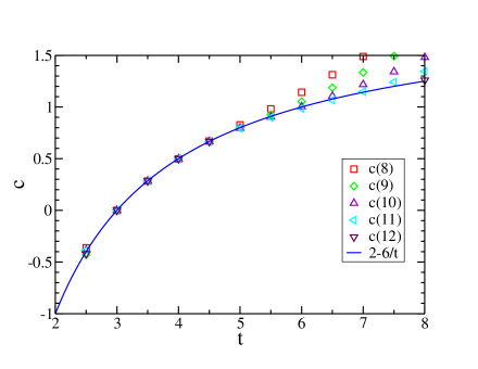
Figure 27: Central charge for the cluster model on the triangular lattice. The transfer direction is perpendicular to a line of $N$ Potts spins. All fits are for $N$ which have the same remainder modulo 3 (otherwise deviations from the expected result $c=2-\frac{6}{t}$ will appear close to $Q=0$ and $Q=4$).

To test this heuristic argument, let us consider the case of the triangular lattice. Setting $v={\rm e}^{K}-1$, the Potts model is integrable when $v^{3}+3v^{2}=Q$ [34]. When $Q\in[0,4]$ this describes three branches. The upper one is the ferromagnetic transition, of course, and by analytic continuation the middle one should then govern the Berker-Kadanoff phase. The remaining lower branch is thus a natural candidate for one of the two antiferromagnetic transition lines. Numerics for the central charge of the cluster model along the lower branch is shown in Fig. 27 and is indeed well described by $c=2-\frac{6}{t}$. The same results of course hold by duality for the model on the hexagonal lattice.

Acknowledgments: J. L. Jacobsen thanks J.-F. Richard, J. Salas, and A. Sokal for related collaborations, and SPhT for their warm hospitality.

Appendix A Block spins and the $Q=0$ case

We use for instance the $osp(2/2)$ $\check{R}$ matrix given in [35]. In the latter reference, a more general expression is given for the $q$-deformed case. We take the limit $q\rightarrow 1$. At the same time we scale the spectral parameter $x=e^{i\gamma v}$, $q={\rm e}^{i\gamma}$, with $\gamma\rightarrow 0$. We then obtain the expression

$$\check{R}=P_{1}+{2+v\over 2-v}\,P_{0}-\sqrt{2}{4v\over(v-2)^{2}}\,P_{N}$$ (72)

The $R$ matrix acts in the tensor product of two fundamental, four-dimensional representations. The basis states in the latter are the bosonic states $|1\rangle$, $|4\rangle$ and the fermionic states $|2\rangle$, $|3\rangle$. The projectors are as follows:

$(i)$ One-dimensional blocks:

$$P_{1}=1,\quad P_{0}=0,\quad P_{N}=0,\qquad\hbox{ for }|1\rangle\otimes|1\rangle\hbox{ and }|4\rangle\otimes|4\rangle$$

$$P_{1}=0,\quad P_{0}=1,\quad P_{N}=0,\qquad\hbox{ for }|2\rangle\otimes|2\rangle\hbox{ and }|3\rangle\otimes|3\rangle$$ (73)

$(ii)$ Two-dimensional blocks:

$$P_{0}={1\over 2}\left(\begin{array}[]{cc}1&-1\\ -1&1\end{array}\right),\quad P_{1}={1\over 2}\left(\begin{array}[]{cc}1&1\\ 1&1\end{array}\right),\quad P_{N}=0$$ (74)

for the four pairs of states

$$\big{(}|1\rangle\otimes|2\rangle,|2\rangle\otimes|1\rangle\big{)},\ \big{(}|1\rangle\otimes|3\rangle,|3\rangle\otimes|1\rangle\big{)},\ \big{(}|2\rangle\otimes|4\rangle,|4\rangle\otimes|2\rangle\big{)},\ \big{(}|3\rangle\otimes|4\rangle,|4\rangle\otimes|3\rangle\big{)}$$ (75)

and finally

$(iii)$ four-dimensional blocks

$$P_{0} = {1\over 4}\left(\begin{array}[]{cccc}2&0&0&-2\\ 0&2&2&0\\ 0&2&2&0\\ -2&0&0&2\end{array}\right)$$ (80)

$$P_{1} = {1\over 4}\left(\begin{array}[]{cccc}2&0&0&2\\ 0&2&-2&0\\ 0&-2&2&0\\ 2&0&0&2\end{array}\right)$$ (85)

$$P_{N} = {\sqrt{2}\over 4}\left(\begin{array}[]{cccc}1&1&1&-1\\ -1&-1&-1&1\\ -1&-1&-1&1\\ -1&-1&-1&1\end{array}\right)$$ (90)

for the basis states

$$\big{(}|1\rangle\otimes|4\rangle,|2\rangle\otimes|3\rangle,|3\rangle\otimes|2\rangle,|4\rangle\otimes|1\rangle\big{)}.$$ (91)

Consider now a different problem where spins $1/2$ interact with the well-known six-vertex model $\check{R}$ matrix with anisotropy parameter $\gamma$. For the value $u$ of the spectral parameter the Boltzmann weights are represented in Fig. 28, with

$$w_{1} = w_{2}=1$$

$$w_{3} = w_{4}={\sin u\over\sin(\gamma+u)}$$

$$w_{5} = {\lambda\sin\gamma\over\sin(\gamma+u)}\,{\rm e}^{iu},\quad w_{6}={\lambda^{-1}\sin\gamma\over\sin(\gamma+u)}\,{\rm e}^{-iu}$$ (92)

where $\lambda$ is a parameter at our disposal (a gauge parameter), and for $\lambda=1$ the $\check{R}$ matrix commutes with $su(2)_{q}$, with $q=e^{i\gamma}$.

Figure 28: Weights in the six-vertex model.

We now consider the following situation. Take a square lattice, and with every horizontal line associate the parameters $h,h+{\pi\over 2}$ in alternance. With the vertical lines, associate similarly the parameters $v,v+{\pi\over 2}$ in alternance (see Fig. 29). The weights at the vertices are given by the foregoing six-vertex formula with $u$ being the difference of the horizontal parameter and the vertical parameter for the two intersecting lines. Since the Boltzmann weights are invariant under a shift of $u$ by $\pi$, we end up with two kinds of vertices, those for which $u=h-v$ and those for which $u=h-v\pm{\pi\over 2}$.

Figure 29: Staggered vertex model, with alternating parameters on horizontal and vertical lines.

We now consider interaction blocks where a pair of horizontal lines meets a pair of vertical lines. We use these blocks to define a new interaction matrix, where each link can carry four states, made out of the two spins $1/2$ of the block. In the limit $q\rightarrow i$ ($\gamma\rightarrow{\pi\over 2}$), the interaction becomes trivial at fixed $u$, but if we let at the same time $u$ approach zero as

$$\gamma = {\pi\over 2}+\epsilon$$

$$u = \epsilon w$$ (93)

we claim that we obtain, after inserting appropriate gauge factors, the $osp(2/2)$ $\check{R}$ matrix, with the following correspondences

$$|++\rangle \equiv |1\rangle$$

$$|+-\rangle+i\,|-+\rangle \equiv |2\rangle$$

$$|+-\rangle-i\,|-+\rangle \equiv |3\rangle$$

$$|--\rangle \equiv |4\rangle$$ (94)

together with $v=-2w$.

The check is laborious. We give here a simple example based on the fact that

$$\check{R}_{osp}(|1\rangle\otimes|4\rangle)=-{4(v-1)\over(v-2)^{2}}\,|1\rangle\otimes|4\rangle+{v^{2}\over(v-2)^{2}}\,|4\rangle\otimes|1\rangle$$

$$+{2v\over(v-2)^{2}}\,(|2\rangle\otimes|3\rangle+|3\rangle\otimes|2\rangle)$$ (95)

This leads among others to the two vertices represented in Fig. 30. These vertices are obtained in turn as a sum over configurations of the spins $1/2$. For the first, one has the weight

$$\left({\sin u\over\sin(\gamma+u)}\right)^{2}\left({\cos u\over\cos(\gamma+u)}\right)^{2}\rightarrow{w^{2}\over(w+1)^{2}}$$

and for the second

$${\sin^{2}\gamma\over\sin^{2}(\gamma+u)}{\rm e}^{2iu}-{\sin^{2}\gamma\sin^{2}u\over\sin^{2}(\gamma+u)\cos^{2}(\gamma+u)}{\rm e}^{2iu}\rightarrow 1-{w^{2}\over(w+1)^{2}}={1+2w\over(1+w)^{2}}$$

in agreement with the matrix elements from $\check{R}_{osp}$.

Figure 30: Two examples of the equivalence between $\check{R}$ matrix elements. Diagrams on the left are $osp$ vertices together with their Boltzmann weight, and they are obtained from the corresponding “microscopic” configurations on the right.

It is interesting to notice that as $q\rightarrow i$, the tensor product of two fundamental representations of $su(2)_{q}$, which decomposes as the sum of a one- and a three-dimensional representation like for $q=1$ when $q$ is generic, becomes indecomposable, and has the structure shown in Fig. 31, where $|u_{1}\rangle=e^{i\pi/4}|+-\rangle+e^{-i\pi/4}|-+\rangle$ and $|u_{2}\rangle=e^{-i\pi/4}|+-\rangle+e^{i\pi/4}|-+\rangle$, and the arrows indicate the action of the $su(2)_{q}$ generators:

$$S^{-}=q^{\sigma^{z}}\otimes\sigma^{-}+\sigma^{-}\otimes q^{-\sigma^{z}}$$

$$S^{+}=q^{\sigma^{z}}\otimes\sigma^{+}+\sigma^{+}\otimes q^{-\sigma^{z}}$$ (96)

Figure 31: Indecomposable representation $1/2^{\otimes 2}$ for $q=i$.

It turns out that, if one introduces the other generators

$$\tilde{S}^{-}=q^{-\sigma^{z}}\otimes\sigma^{-}+\sigma^{-}\otimes q^{\sigma^{z}}$$

$$\tilde{S}^{+}=q^{-\sigma^{z}}\otimes\sigma^{+}+\sigma^{+}\otimes q^{\sigma^{z}}$$ (97)

at $q=i$, together with the limits $\lim_{q\rightarrow i}{(S^{\pm})^{2}\over q+q^{-1}}$, one obtains the four-dimensional representation of $osp(2/2)$.

References

- [1] P.P. Martin, “Potts models and related problems in statisticals mechanics” (World Scientific, Singapore, 1991).
- [2] H. Saleur, Nucl. Phys. B 360, 219 (1991).
- [3] V. Pasquier and H. Saleur, Nucl. Phys. B 330, 523 (1990).
- [4] F. Essler, H. Frahm and H. Saleur, Nucl. Phys. B 712, 513 (2005) [cond-mat/0501197].
- [5] J.L. Jacobsen, N. Read and H. Saleur, Phys. Rev. Lett. 90, 090601 (2003) [cond-mat/0205033].
- [6] J.L. Jacobsen, J. Salas and A.D. Sokal, J. Stat. Phys. 119, 1153-1281 (2005) [cond-mat/0401026].
- [7] P.W. Kasteleyn and C.M. Fortuin, J. Phys. Soc. Jap. Suppl. 26, 11 (1969).
- [8] C.M. Fortuin and P.W. Kasteleyn, Physica 57, 536 (1972).
- [9] P. Di Francesco, H. Saleur and J.B. Zuber, J. Stat. Phys. 49, 57 (1987).
- [10] J.L. Jacobsen and J. Salas, J. Stat. Phys. (in print) [cond-mat/0407444].
- [11] R.J. Baxter, S.B. Kelland and F.Y. Wu, J. Phys. A 9, 397 (1976).
- [12] N. Read and H. Saleur, Nucl. Phys. B 613, 409 (2001) [hep-th/0106124].
- [13] R.J. Baxter, Proc. Roy. Soc. London 383, 43 (1982).
- [14] R.J. Baxter, Studies in Appl. Math. 50, 51 (1971).
- [15] N.Yu. Reshetikhin and H. Saleur, Nucl. Phys. B 419, 507 (1994) [hep-th/9309135].
- [16] F.C. Alcaraz, M.N. Barber and M.T. Batchelor, Ann. Phys. (NY) 182, 280 (1988).
- [17] H. de Vega and E. Lopes, Nucl. Phys. B 362, 261 (1991).
- [18] J.L. Jacobsen and H. Saleur, Nucl. Phys. B 716, 439 (2005) [cond-mat/0502052].
- [19] I. Affleck, in Fields, strings and critical phenomena, Les Houches, 1988, edited by E. Brézin and J. Zinn-Justin (Elsevier Science Publishers, Amsterdam, 1989).
- [20] V. Pasquier, J. Phys. A 20, L1229 (1987).
- [21] G.E. Andrews, R.J. Baxter and P.J. Forrester, J. Stat. Phys. 35, 193 (1984).
- [22] D. Huse, Phys. Rev. B 30, 3908 (1984).
- [23] A.B. Zamolodchikov and V.A. Fateev, Sov. Phys. JETP 62, 215 (1985).
- [24] T. Jayaraman, K.S. Narain and M.H. Sarmadi, Nucl. Phys. B 343, 418 (1990).
- [25] D. Gepner and Z. Qiu, Nucl. Phys. B 285, 423 (1987).
- [26] J. Distler and Z. Qiu, Nucl. Phys. B 336, 533 (1990).
- [27] G. Felder, Nucl. Phys. B 317, 215 (1989); erratum ibid. 324, 548 (1989).
- [28] V. Fateev and Al. Zamolodchikov, Sov. Phys. JETP 63, 913 (1986).
- [29] V. Fateev and Al. Zamolodchikov, Phys. Lett. B 271, 91 (1991).
- [30] V. Fateev, Nucl. Phys. B 473, 509 (1996).
- [31] M. Asorey, J.G. Esteve and J. Salas, Phys. Rev. B 48, 3626 (1993) [hep-th/9211048].
- [32] B. Nienhuis, Phys. Rev. Lett. 49, 1062 (1982).
- [33] A.M.M. Pruisken, M.A. Baranov and M. Voropaev, Phys. Rev. Lett. 505, 4432 (2003) [cond-mat/0101003].
- [34] R.J. Baxter, H.N.V. Temperley and S.E. Ashley, Proc. Roy. Soc. A 358, 535 (1978).
- [35] Z. Bassi and A. Leclair, Nucl. Phys. B 578, 577 (2000) [hep-th/9911105].