Nonlinear dynamics in one dimension:
On a criterion for coarsening and its temporal law

Abstract

We develop a general criterion about coarsening for a class of nonlinear evolution equations describing one dimensional pattern-forming systems. This criterion allows one to discriminate between the situation where a coarsening process takes place and the one where the wavelength is fixed in the course of time. An intermediate scenario may occur, namely ‘interrupted coarsening’. The power of the criterion on which a brief account has been given [P. Politi and C. Misbah, Phys. Rev. Lett. 92 , 090601 (2004)], and which we extend here to more general equations, lies in the fact that the statement about the occurrence of coarsening, or selection of a length scale, can be made by only inspecting the behavior of the branch of steady state periodic solutions. The criterion states that coarsening occurs if $\lambda^{\prime}(A)>0$ while a length scale selection prevails if $\lambda^{\prime}(A)<0$, where $\lambda$ is the wavelength of the pattern and $A$ is the amplitude of the profile (prime refers to differentiation). This criterion is established thanks to the analysis of the phase diffusion equation of the pattern. We connect the phase diffusion coefficient $D(\lambda)$ (which carries a kinetic information) to $\lambda^{\prime}(A)$, which refers to a pure steady state property. The relationship between kinetics and the behavior of the branch of steady state solutions is established fully analytically for several classes of equations. Another important and new result which emerges here is that the exploitation of the phase diffusion coefficient enables us to determine in a rather straightforward manner the dynamical coarsening exponent. Our calculation, based on the idea that $|D(\lambda)|\sim\lambda^{2}/t$, is exemplified on several nonlinear equations, showing that the exact exponent is captured. We are not aware of another method that so systematically provides the coarsening exponent. Contrary to many situations where the one dimensional character has proven essential for the derivation of the coarsening exponent, this idea can be used, in principle, at any dimension. Some speculations about the extension of the present results are outlined.

I Introduction

Pattern formation is ubiquitous in nature, and especially for systems which are brought away from equilibrium. Examples are encountered in hydrodynamics, reaction-diffusion systems, interfacial problems, and so on. There is now an abundant literature on this topic cross93 ; patterns_book . Generically, the first stage of pattern formation is the loss of stability of the homogeneous solution against a spatially periodic modulation. This generally occurs at a critical value of a control parameter, $\mu=\mu_{c}$ (where $\mu$ stands for the control parameter) and at a critical wavenumber $q=q_{c}$. The dispersion relation about the homogeneous solution (where perturbations are sought as $e^{iqx+\omega t}$), in the vicinity of the critical point assumes, in most of pattern-forming systems, the following parabolic form (Fig. 1, inset)

$$\omega=\delta-(q-q_{c})^{2}$$ (1)

where $\delta$ is proportional to $(\mu-\mu_{c})$. For $\delta<0$, $\omega<0$ for all $q^{\prime}s$ and the homogeneous state is stable. Conversely, for $\delta>0$ there is a band of wavevectors $\Delta q\equiv(q-q_{c})=\pm\sqrt{\delta}$ corresponding to unstable modes (Fig. 1), so that infinitesimal perturbations grow exponentially with time until nonlinear effects can no longer be ignored. In the vicinity of the bifurcation point ($\delta=0$) only the principal harmonic with $q=q_{c}$ is unstable, while all other harmonics are stable. For example, Rayleigh-Bénard convection, Turing systems, and so on, fall within this category, and their nonlinear evolution equation is universal in the vicinity of the bifurcation point. If the field of interest (say a chemical concentration) is written as $A(x,t)e^{iq_{c}x}$, where $A$ is a complex slowly varying amplitude, then $A$ obeys the canonical equation

$$\partial_{t}A=A+\partial_{xx}A-|A|^{2}A$$ (2)

where it is supposed that the coefficient of the cubic term is negative to ensure a nonlinear saturation. Because the band of active modes is narrow and centered around the principal harmonic, no coarsening can occur, and the pattern will select a given length, which is often close to that of the linearly fastest growing mode. However, the amplitude equation above exhibits a phase instability, known under the Eckhaus instability cross93 , stating that among the band of allowed states, $|\Delta q|=\sqrt{\delta}$, only those modes whose wavevectors satisfy $|\Delta q|<\sqrt{\delta/3}$ are stable with respect to a wavelength modulation.

There are many other situations where the bifurcation wavenumber $q_{c}\rightarrow 0$ and therefore a separation of a slow amplitude and a fast oscillation is illegitimate. Contray to the case (1), where the field can be written as $A(x,t)e^{iq_{c}x}$ with $A$ being supposed to vary slowly in space and time, if $q_{c}\to 0$ the supposed fast oscillation, $e^{iq_{c}x}$, becomes slow as well and a separation of $A$ does not make a sense anymore. In this case, a generic form of the dispersion relation is (Fig. 2, main)

$$\omega=\delta q^{2}-q^{4}.$$ (3)

A third situation is the one where the dispersion relation takes the form (Fig. 2, inset)

$$\omega=\delta-q^{2}.$$ (4)

In both cases, Eqs. (3,4), the instability occurs for $\delta>0$, and the band of unstable modes extends from $q=0$ to $q=\sqrt{\delta}$. That is to mean, there is an infinite number of unstable harmonics: if $\bar{q}$ is the wavenumber of an unstable mode, then also $\bar{q}/2,\bar{q}/3,\dots$ are unstable. Examples that fall in this category are numerous Misbah94 : the air-liquid interface in a thin film falling on an inclined plane, flame fronts, step dynamics in step flow growth, sand ripples, and so on, or simply the Ginzburg-Landau equation (2), which corresponds to case (4).

Dispersion relation (3) has an extra factor of $q^{2}$ which is often due to a conservation constraint (see also below). Because of the dispersion form, constant plus a quadratic term, (4) might formally resemble (1). However, an important caution must be taken: in (1) it must be remembered that $q$ should remain close to $q_{c}$, so that only one harmonic is active, while in (4) no such a restriction is made, and therefore $q$ can be as close as possible to zero, leading to a highly nonlinear dynamics.

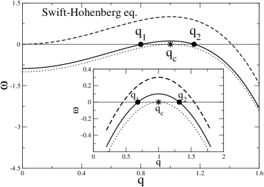
Figure 1: Inset: Dispersion curve (1): $\omega=\delta-(q-q_{c})^{2}$. There is loss of stability at a critical wavenumber $q_{c}$, when $\delta=0$ (dotted line). For $\delta>0$, the unstable band extends from $q=q_{1}$ to $q=q_{2}$ (full line). With increasing $\delta$ the unstable region widens (dashed line). The parabolic shape of $\omega(q)$ is an approximation, valid close to its maximum. This applies, e.g., to the dispersion curve (38) of the Swift-Hohenberg eq. (see the main figure): $\omega=\delta-(1-q^{2})^{2}$ [$q_{c}=1$]. When $\delta=1$ (dashed line) the unstable band extends down to $q=0$ and $\omega(q)$ resembles the dispersion curve of the Cahn-Hilliard eq. (see (3) and Fig. 2).

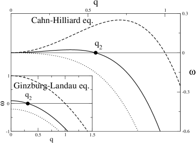
Figure 2: Main: dispersion curve (3), valid, e.g., for the Cahn-Hilliard equation: $\omega=\delta q^{2}-q^{4}$. Dotted line: below threshold ($\delta<0$). Full line: just above threshold. Dashed line: well above threshold. The vanishing of $\omega(0)$ for any $\delta$ is a consequence of the traslational invariance of the CH eq. in the ‘growth’ direction. Inset: The Ginzburg-Landau eq. is one case where such invariance is absent and the dispersion curve has the form (4): $\omega=\delta-q^{2}$.

Other types of dispersion relations which may arise, and which are worth of mention, correspond to situations where $\omega=\delta|q|-q^{2}$, or $\omega=\delta|q|-|q|^{3}$, leading also to a vigorous mode mixing, for the same reasons evoked above. The occurrence of a non analytic dispersion relation with $|q|$ is a consequence of long range interactions Kassner02 . If the unstable band extends down to $q=0$, the appropriate form of the evolution equation is not an amplitude equation for a slowly varying function $A$, but rather a partial nonlinear differential equation, or an integro-differential equation, for the full field of interest, say $h(x,t)$ if one has in mind a front profile.

A prominent example of a partial differential equation is the Kuramoto-Sivashinsky Nepo ; Kuramoto ; Sivashinsky (KS) equation

$$\partial_{t}u=-\partial_{xx}u-\partial_{xxxx}u+u\partial_{x}u$$ (5)

which leads to spatio-themporal chaos. Note that by setting $u=\partial_{x}h$ we obtain an equivalent form of this equation, namely $\partial_{t}h=-\partial_{xx}h-\partial_{xxxx}h+(\partial_{x}h)^{2}/2$. This equation arises in several contexts: liquid films flowing down an inclined plane Nepo , flame fronts Sivashinsky , step flow growth of a crystal surface Misbah94 .

Complex dynamics such as chaos, coarsening, etc $\dots$, are naturally expected if modes of arbitrarily large wavelength are unstable. However, these dynamics may occur for systems characterized by the dispersion relation (1) as well, if the system is further driven away from the critical point (i.e., if $q_{2}\gg q_{1}$, see Fig. 1) because higher and higher harmonics become active. We may expect, for example, coarsening to become possible up to a total wavelength of the order of $2\pi/q_{1}$.

For systems which are at global equilibrium the nonlinearity $u\partial_{x}u$ is not allowed, and a prototypical equation having the dispersion relation (3) is the Cahn-Hilliard equation

$$\partial_{t}u=-\partial_{xx}[u+\partial_{xx}u-u^{3}].$$ (6)

The linear terms are identical to the KS one, and the difference arises from the nonlinear term. Note that if dynamics is not subject to a conservation constraint, $(-\partial_{xx})$ on the right hand side is absent, and the dispersion relation is given by Eq. (4). The resulting equation is given by (2) for a real $A$ and it is called real Ginzburg-Landau (GL) equation or Allen-Cahn equation.

The KS equation, or its conserved form (obtained by applying $\partial_{xx}$ on the right hand side), was suspected for a long time to arise as the generic nonlinear evolution equation for nonequilibrium systems (the quadratic term is non variational in that it can not be written as a functional derivative) whenever a dispersion relation is of type (3). Several recent studies, especially in Molecular Beam Epitaxy (MBE), have revealed an increasing evidence for the occurrence of completely new types of equations, with a variety of dynamics: besides chaos, there are ordered multisoliton Misbah96 ; Sato96 solutions, coarsening Review , freezing of the wavelength accompanied by a perpetual increase of the amplitude OPL . Moreover, equations bearing strong resemblance with each other Paulin exhibit a completely different dynamics. Thus it is highly desirable to extract some general criteria that allow one to discriminate between various dynamics.

A central question that has remained open so far, and which has been the subject of a recent brief exposition Politi04 , was the understanding of the general conditions under which dynamics should lead to coarsening, or rather to a selection of a length scale. In this paper we shall generalize our proof presented in Politi04 to a larger number of classes of nonlinear equations, for which the same general criterion applies: the sign of the phase diffusion coefficient $D$ is linked to a property of the steady state branch. More precisely, the sign of $D$ is shown to be the opposite of the sign of $\lambda^{\prime}(A)$, the derivative of the wavelength $\lambda$ of the steady state with respect its amplitude $A$. Therefore, coarsening occurs if (and only if) the wavelength increases with the amplitude.

Another important new feature that constitutes a subject of this paper, is the fact that the exploitation of the phase diffusion coefficient $D(\lambda)$ will allow us to derive analytically the coarsening exponent, i.e. the law according to which the wavelength of the pattern increases in time. For all known nonlinear equations whose dispersion relation has the form (3) or (4) and display coarsening, we have obtained the exact value of the coarsening exponent, and we predict exponents for other non exploited yet equations. An important point is that this is expected to work at any dimension. Indeed, the derivation of the phase equation can be done in higher dimension as well. If our criterion, based on the idea that $|D(\lambda)|\sim\lambda^{2}/t$, remains valid at higher dimensions, it should become a precious tool for a straightforward derivation of the coarsening exponent at any dimension.

II The phase equation method

II.1 Generality

Coarsening of an ordered pattern occurs if steady state periodic solutions are unstable with respect to wavelength fluctuations. The phase equation method Kevorkian allows to study in a perturbative way the modulations of the phase $\phi$ of the pattern. For a periodic structure of period $\lambda$, $\phi=qx$, where $q=2\pi/\lambda$ is a constant. If we perturb this structure, $q$ acquires a space and time dependence and the phase $\phi$ is seen to satisfy a diffusion equation, $\partial_{t}\phi=D\partial_{xx}\phi$. The quantity $D$, called phase diffusion coefficient, is a function of the steady state solutions and its sign determines the stable ($D>0$) or unstable ($D<0$) character of a wavelength perturbation.

A negative value of $D$ induces a coarsening process, whose typical time and length scales are related by $|D(\lambda)|\sim\lambda^{2}/t$, as simply derived from the solution of the phase diffusion equation: this relation allows to find the coarsening law $\lambda(t)$. Therefore, the phase equation method not only allows to determine if certain classes of partial differential equations (PDE) display coarsening or not; it also allows to find the coarsening laws, when $D<0$. In the rest of this section, we are going to offer a short exposition of the phase equation method without referring to any specific PDE. Explicit evolution equations will be treated in the next sections, with some calculations relegated to the appendix.

Let us consider a general PDE of the form

$$\partial_{t}u(x,t)=\tilde{\cal N}[u]$$ (7)

where $\tilde{\cal N}$ is an unspecified nonlinear operator, which is assumed not to depend explicitly on space and time. $u_{0}(x)$ is a periodic steady state solution: $\tilde{\cal N}[u_{0}]=0$ and $u_{0}(x+\lambda)=u_{0}(x)$.

When studying the perturbation of a steady state, it is useful to separate a fast spatial variable from slow time and space dependencies. The stationary solution $u_{0}$ does not depend on time and it has a fast spatial dependence, which is conveniently expressed through the phase $\phi=qx$. Once we perturb the stationary solution,

$$u=u_{0}+\epsilon u_{1}+\dots,$$ (8)

the wavevector $q=\partial_{x}\phi$ gets a slow space and time dependence: $q=q(X,T)$, where $X=\epsilon x$ and $T=\epsilon^{\alpha}t$. Because of the diffusive character of the phase variable, the exponent $\alpha$ is equal to two. Space and time derivatives now read

$$\partial_{x} = q\partial_{\phi}+\epsilon\partial_{X}$$ (9a)

$$\partial_{t} = \epsilon(\partial_{T}\psi)\partial_{\phi}$$ (9b)

where the second order term in the latter equation ($\epsilon^{2}\partial_{T}$) has been neglected. Finally, along with the phase $\phi$ it is useful to introduce the slow phase $\psi(X,T)=\epsilon\phi(x,t)$, so that $q=\partial_{X}\psi$.

Replacing the $u-$expansion (8) and the derivates (9) with respect to the new variables in Eq. (7), we find an $\epsilon-$expansion which must be vanished term by term. The zero order equation is trivial, $\tilde{\cal N}_{0}[u_{0}]=0$: this equation is just the rephrasing of the time-independent equation in terms of the phase variable $\phi$ (the subscript in $\tilde{\cal N}_{0}$ means that Eqs. (9) have been applied at zero order in $\epsilon$, i.e. $\partial_{x}=q\partial_{\phi}$).

The first order equation is more complicated, because both the operator $\tilde{\cal N}$ and the solution $u$ are $\epsilon-$expanded. On very general grounds, we can rewrite $\partial_{t}u(x,t)=\tilde{\cal N}[u]$ as

$$\epsilon(\partial_{T}\psi)\partial_{\phi}u_{0}=(\tilde{\cal N}_{0}+\epsilon\tilde{\cal N}_{1})[u_{0}+\epsilon u_{1}]$$ (10)

where $\tilde{\cal N}_{1}$ comes from first order contributions to the derivatives (9). If we use the Fréchet derivative Zwillinger , $\tilde{\cal L}_{0}$, defined through the relation

$$\tilde{\cal N}_{0}[u_{0}+\epsilon u_{1}]=\tilde{\cal N}_{0}[u_{0}]+\epsilon\tilde{\cal L}_{0}[u_{1}]+O(\epsilon^{2})$$ (11)

we get

$$\tilde{\cal L}_{0}[u_{1}]=(\partial_{T}\psi)\partial_{\phi}u_{0}-\tilde{\cal N}_{1}[u_{0}]\equiv g(u_{0},q,\psi).$$ (12)

At first order, therefore, we get an heterogeneous linear equation (the Fréchet derivative of a nonlinear operator is linear). The translational invariance of the operator $\tilde{\cal N}$ guarantees that $\partial_{\phi}u_{0}$ is solution of the homogeneous equation: according to the Fredholm alternative theorem Fredholm , a solution for the heterogeneous equation may exist only if $g$ is orthogonal to the null space of the adjoint operator $\tilde{\cal L}^{\dagger}$. In simple words, if $\tilde{\cal L}^{\dagger}[v]=0$, $v$ and $g$ must be orthogonal. This condition, see Eq. (12), reads

$$\langle v,\partial_{\phi}u_{0}\rangle\partial_{T}\psi=\langle v,\tilde{\cal N}_{1}[u_{0}]\rangle,$$ (13)

where $\langle f,g\rangle=(2\pi)^{-1}\int_{0}^{2\pi}d\phi f^{*}g$.

It happens that $\tilde{\cal N}_{1}[u_{0}]$ is proportional to $\partial_{X}q=\partial_{X\hbox{\hskip-2.84544pt}X}\psi$, and the previous equation has the form of a diffusion equation for the phase $\psi$,

$$\partial_{t}\psi=D\partial_{X\hbox{\hskip-2.84544pt}X}\psi.$$ (14)

II.2 Applications

II.2.1 The generalized Ginzburg-Landau equation

The (real) Ginzburg-Landau equation is written as

$$\partial_{t}u=(u-u^{3})+u_{xx}$$ (15)

whose linear spectrum, for an excitation $u(x,t)=\exp(\omega t+iqx)$ is $\omega(q)=1-q^{2}$. This equation is the prototype for the evolution of a nonconserved order parameter with two equivalent stable solutions, $u=\pm 1$. Starting from the trivial solution $u=0$, we have a linear instability leading to a logarithmically slow coarsening process Langer .

This equation can be easily generalized to

$$\partial_{t}u=B(u)+G(u)\,u_{xx}\;,$$ (16)

which will therefore be called generalized Ginzburg-Landau (gGL) equation. If $B(u)\simeq u$ and $G(u)\simeq 1$ for small $u$, the linear spectrum is unmodified, but the nonlinear behavior can be totally different, depending on the full (positive) expressions of $B(u)$ and $G(u)$. Steady states are determined by the relation $u_{0}^{\prime\prime}(x)=-B(u_{0})/G(u_{0})$, so they correspond to the trajectories of a classical particle moving under the force $-B(u_{0})/G(u_{0})$.

Now, let us apply the expansions (8) for the order parameter and (9) for the derivatives to Eq. (16). The first and second spatial derivatives can also be written as

$$\partial_{x} = q\partial_{\phi}+\epsilon\psi_{X\hbox{\hskip-2.84544pt}X}\partial_{q}$$ (17a)

$$\partial_{xx} = q^{2}\partial_{\phi\phi}+\epsilon\psi_{X\hbox{\hskip-2.84544pt}X}(2q\partial_{q}+1)\partial_{\phi}$$ (17b)

As anticipated in the previous section, the zero and first order equations read $\tilde{\cal N}_{0}[u_{0}]=0$ and $\tilde{\cal L}_{0}[u_{1}]=g$, where

$$\tilde{\cal N}_{0}[u_{0}]=B(u_{0})+G(u_{0})q^{2}\partial_{\phi\phi}u_{0}$$ (18)

is the nonlinear operator defining the gGL equation,

$$\tilde{\cal L}_{0}[u_{1}]=[B^{\prime}(u_{0})+G^{\prime}(u_{0})q^{2}(\partial_{\phi\phi}u_{0})+G(u_{0})q^{2}\partial_{\phi\phi}]u_{1}$$ (19)

is its Fréchet derivative, and

$$g=(\partial_{T}\psi)\partial_{\phi}u_{0}-(\partial_{X\hbox{\hskip-2.84544pt}X}\psi)G(u_{0})(2q\partial_{q}+1)\partial_{\phi}u_{0}\;.$$ (20)

Because of translational invariance, $\tilde{\cal L}_{0}[\partial_{\phi}u_{0}]=0$. Its adjoint is easily found to be

$$\tilde{\cal L}^{\dagger}_{0}[v]=q^{2}\partial_{\phi\phi}[vG(u_{0})]+[B^{\prime}(u_{0})+G^{\prime}(u_{0})q^{2}(\partial_{\phi\phi}u_{0})]v.$$ (21)

If we define $w=vG(u_{0})$, the equation $\tilde{\cal L}^{\dagger}_{0}[v]=0$ is identical to $\tilde{\cal L}_{0}[w]=0$, so that we can choose $w=\partial_{\phi}u_{0}$ and $v=\partial_{\phi}u_{0}/G(u_{0})$.

The orthogonality condition between $v$ and $g$ reads

$$(\partial_{T}\psi)\langle v,\partial_{\phi}u_{0}\rangle-(\partial_{X\hbox{\hskip-2.84544pt}X}\psi)\langle v,G(u_{0})(2q\partial_{q}+1)\partial_{\phi}u_{0}\rangle=0$$ (22)

and replacing the explicit expression for $v$, we get the phase diffusion equation

$$\partial_{T}\psi=D\partial_{X\hbox{\hskip-2.84544pt}X}\psi$$ (23)

with

$$D=\frac{\partial_{q}\langle q(\partial_{\phi}u_{0})^{2}\rangle}{\left\langle{(\partial_{\phi}u_{0})^{2}\over G(u_{0})}\right\rangle}\equiv{D_{1}\over D_{2}}.$$ (24)

Assuming a positive $G$, the sign of $D$ is fixed by the increasing or decreasing character of $\langle q(\partial_{\phi}u_{0})^{2}\rangle$ with the wavevector $q$. Reversing to the old variable $x$,

$$\langle q(\partial_{\phi}u_{0})^{2}\rangle={1\over 2\pi}\int_{0}^{\lambda}dx(u_{0}^{\prime})^{2}={J\over 2\pi}$$ (25)

where $J$ is the well known action variable, whose derivative with respect to the ‘energy’ of the particle gives the period $\lambda$. The following relations are easily established:

$$D_{1}={1\over 2\pi}{\partial J\over\partial q}=-{\lambda^{3}\over 4\pi^{2}}\left({\partial\lambda\over\partial E}\right)^{-1}=-{\lambda^{3}\over 4\pi^{2}}{B(A)\over G(A)}\left({\partial\lambda\over\partial A}\right)^{-1}$$ (26)

where $A$ is the amplitude of the oscillation, i.e. the (positive) maximal value for $u_{0}(x)$.

If $G(u)\equiv 1$, a compact formula for $D$ is

$$D=-{\lambda^{2}B(A)\over J(\partial_{A}\lambda)}~{}~{}~{}~{}G(A)\equiv 1.$$ (27)

In conclusion, a coarsening process occurs ($D<0$) if the wavelength of the steady states increases with increasing their amplitude. In App. A we make some general remarks on the behavior of $\lambda(A)$ for several different potentials.

II.2.2 The generalized Cahn-Hilliard equation

The Cahn-Hilliard equation is the conserved ‘version’ of the Ginzburg-Landau equation,

$$\partial_{t}u=-\partial_{xx}[(u-u^{3})+u_{xx}].$$ (28)

The spatial average of the order parameter is time independent, $d\langle u\rangle/dt=0$, and the linear spectrum is $\omega(q)=q^{2}-q^{4}$: it therefore has a maximum at a finite value $q_{u}=1/\sqrt{2}$, called the most unstable wavevector. The linear regime corresponds to an exponential unstable growth of such mode, with a rate $\omega(q_{u})$, followed by a logarithmic coarsening.

The above equation can be made of wider application by considering the following generalized Cahn-Hilliard (gCH) equation

$$\partial_{t}u=-C(u)\partial_{xx}[B(u)+G(u)u_{xx}].$$ (29)

In Sec. III.4 we will discuss thoroughly the coarsening of this class of models, because of its relevance for the crystal growth of vicinal surfaces. In that case, the local height $z(x,t)$ of the steps satisfies the equation

$$\partial_{t}z=-\partial_{x}\{B(m)+G(m)\partial_{x}[C(m)\partial_{x}m]\}$$ (30)

where $m=\partial_{x}z$. If we pass to the new variable $u(m)=\int_{0}^{m}dsC(s)$ and take the spatial derivative of the above equation, we get the gCH equation (29). It is worthnoting that steady states are given by the equation $B(u_{0})+G(u_{0})u_{0}^{\prime\prime}=j_{0}$, where $j_{0}$ is a constant determined by the condition $\langle u_{0}\rangle=m_{0}$ that imposes the (conserved) average value of the order parameter. If steps are oriented along a high-symmetry orientation, $m_{0}=0=j_{0}$. In the following we are considering this case only, so the equation determining steady states, $B(u_{0})+G(u_{0})u_{0}^{\prime\prime}=0$, is the same as for the gGL equation.

If we proceed along the lines explained in Sec.II.1 and keep in mind notations used in Sec.II.2.1, the first order equation in the small parameter $\epsilon$ reads

$$-q^{2}\partial_{\phi\phi}\tilde{\cal L}_{0}[u_{1}] =(\partial_{T}\psi){\partial_{\phi}u_{0}\over C(u_{0})}$$

$$+(\partial_{X\hbox{\hskip-2.84544pt}X}\psi)q^{2}\partial{\phi\phi}[G(u_{0})(2q\partial_{q}+1)\partial_{\phi}u_{0}].$$

According to the Fredholm alternative theorem, the right hand side must be orthogonal to the solution $v$ of the equation

$$(\partial_{\phi\phi}\tilde{\cal L}_{0})^{\dagger}[v]=\tilde{\cal L}_{0}^{\dagger}\partial_{\phi\phi}v=0.$$ (32)

According to the results of the previous section, we know that $\partial_{\phi\phi}v=(\partial_{\phi}u_{0})/G(u_{0})$. The orthogonality condition now reads

$$\left\langle v,{\partial_{\phi}u_{0}\over C(u_{0})}\right\rangle(\partial_{T}\psi)$$

$$+ q^{2}\langle v,\partial{\phi\phi}[G(u_{0})(2q\partial_{q}+1)\partial_{\phi}u_{0}]\rangle(\partial_{X\hbox{\hskip-2.84544pt}X}\psi)=0.$$

The quantity multiplying $(\partial_{X\hbox{\hskip-2.84544pt}X}\psi)$ can be rewritten as

$$\langle v,\partial{\phi\phi}[G(u_{0})(2q\partial_{q}+1)\partial_{\phi}u_{0}\rangle =$$

$$\langle{\partial_{\phi}u_{0}\over G(u_{o})},G(u_{0})(2q\partial_{q}+1)\partial_{\phi}u_{0}\rangle =$$

$$\partial_{q}\langle q(\partial_{\phi}u_{0})^{2}\rangle$$ (34)

so we finally have $(\partial_{T}\psi)=D(\partial_{X\hbox{\hskip-2.84544pt}X}\psi)$ with

$$D=-{q^{2}\partial_{q}\langle q(\partial_{\phi}u_{0})^{2}\rangle\over\left\langle v,{\partial_{\phi}u_{0}\over C(u_{0})}\right\rangle}\equiv{q^{2}D_{1}\over\tilde{D}_{2}}.$$ (35)

In App. B we prove that the denominator $\tilde{D}_{2}$ is always positive. If $C$ and $G$ are (positive) constants the proof is straightforward, because $-\langle v\partial_{\phi}u_{0}\rangle=\langle(\partial_{\phi}v)u_{0}\rangle=\langle u_{0}^{2}\rangle$. The diffusion coefficient (35) for the gCH equation is therefore similar to the diffusion coefficient (24) for the nonconserved gGL equation: their sign is determined by the increasing or decreasing character of $\lambda(A)$, the wavelength of the steady state, with respect to its amplitude. The $q^{2}$ term in the numerator of (35) is evidence of the conservation law, i.e., of the second derivative $\partial_{xx}$ in Eq. (29). The denominators $D_{2}$ and $\tilde{D}_{2}$ differ: this is irrelevant for the sign of $D$, but it is relevant for the coarsening law.

If $C(u)\equiv G(u)\equiv 1$, formulas simplify: $D_{1}=-\lambda^{3}B(A)/4\pi^{2}(\partial_{A}\lambda)$ and $\tilde{D}_{2}=\langle u_{0}^{2}\rangle=I/\lambda$, where $I=\oint u_{0}^{2}(x)$ has the same role as $J=\oint(\partial_{x}u_{0})^{2}$ in the nonconserved model. Putting everything together we obtain

$$D=-{\lambda^{2}B(A)\over I(\partial_{A}\lambda)}~{}~{}~{}~{}C(A)\equiv G(A)\equiv 1.$$ (36)

II.2.3 The generalized Swift-Hohenberg equation

Both the (generalized) GL and CH equations have a linear spectrum whose unstable band extends to $q=0$, so that active modes of arbitrarily large wavelength exist. In the Swift-Hohenberg equation we can tune a parameter $\delta$ so that to change the unstable band. The standard form of the equation is

$$\partial_{t}u = \delta u-(1+\partial_{xx})^{2}u-u^{3}$$

$$= -\partial_{x}^{4}u-2\partial_{x}^{2}u-(1-\delta)u-u^{3}$$

Linear stability analysis for a single harmonic $u(x,t)=\exp(\omega t+iqx)$ gives the spectrum

$$\omega(q)=\delta-(1-q^{2})^{2}$$ (38)

and for positive $\delta$ there is a finite unstable band ($\omega(q)>0$) extending from $q_{1}=\sqrt{1-\sqrt{\delta}}$ to $q_{2}=\sqrt{1+\sqrt{\delta}}$. For $\delta=1$, the unstable band is the interval $(0,\sqrt{2})$. The most unstable wavevector is $q_{u}=1$ for any $\delta$. For small $\delta$ the unstable band is narrow; in fact, for $\delta<0.36$, $q_{1}>q_{2}/2$ and period doubling is not allowed. In other words studying coarsening for the Swift-Hohenberg equation close to the threshold $\delta=0$ is not very interesting: nonetheless we will write the phase diffusion equation for any $\delta$ and for a generalized form of the Swift-Hohenberg equation as well.

The zero order equation is easy to write

$$\tilde{\cal N}_{0}[u_{0}]\equiv-q^{4}\partial^{4}_{\phi}u_{0}-2q^{2}\partial^{2}_{\phi}u_{0}-(1-\delta)u_{0}-u_{0}^{3}=0$$ (39)

and the first order equation has the expected form $\tilde{\cal L}_{0}[u_{1}]=g$, where

$$\tilde{\cal L}_{0}\equiv-q^{4}\partial^{4}_{\phi}-2q^{2}\partial^{2}_{\phi}-(1-\delta)-3u_{0}^{2}$$ (40)

is the Fréchet derivative of $\tilde{\cal N}_{0}$ and

$$g\equiv(\partial_{T}\psi)\partial_{\phi}u_{0}$$ (41)

$$+2(\partial_{X\hbox{\hskip-2.84544pt}X}\psi)[(2q^{3}\partial_{q}+3q^{2})\partial^{3}_{\phi}u_{0}+(2q\partial_{q}+1)\partial_{\phi}u_{o}].$$

The operator $\tilde{\cal L}_{0}$ is self-adjoint, so the solution of the homogeneous equation $\tilde{\cal L}_{0}^{\dagger}[v]=0$ is immediately found, because of the translational invariance of $\tilde{\cal N}_{0}$ along $x$: $v=\partial_{\phi}u_{0}$. We therefore have

$$(\partial_{T}\psi)\langle(\partial_{\phi}u_{0})^{2}\rangle=$$ (42)

$$-(\partial_{X\hbox{\hskip-2.84544pt}X}\psi)[\langle\partial_{\phi}u_{0}(4q^{3}\partial_{q}+6q^{2})\partial^{3}_{\phi}u_{0}\rangle$$

$$+2\langle\partial_{\phi}u_{0}(2q\partial_{q}+1)\partial_{\phi}u_{0}\rangle].$$

It is easy to check that both terms appearing in square brackets on the right hand side can be written as $\partial_{q}(\dots)$:

$$\langle\partial_{\phi}u_{0}(4q^{3}\partial_{q}+6q^{2})\partial^{3}_{\phi}u_{0}\rangle = -\partial_{q}\langle 2q^{3}(\partial^{2}_{\phi}u_{0})^{2}\rangle$$ (43a)

$$\langle\partial_{\phi}u_{0}(2q\partial_{q}+1)\partial_{\phi}u_{0}\rangle] = \partial_{q}\langle q(\partial_{\phi}u_{0})^{2}\rangle$$ (43b)

so that the phase diffusion coefficients reads

$$D={\partial_{q}[2q^{3}\langle(\partial^{2}_{\phi}u_{0})^{2}\rangle-2q\langle(\partial_{\phi}u_{0})^{2}\rangle]\over\langle(\partial_{\phi}u_{0})^{2}\rangle}.$$ (44)

Now let us generalize this result to the equation

$$\partial_{t}u=\sum_{n>0}c_{n}\partial_{x}^{n}u+P(u)$$ (45)

where $n$ is assumed even and $P(u)$ an odd function, in order to preserve the symmetries $x\to-x$ and $u\to-u$. Therefore $n=2k$, with $k\geq 1$. We report here only the final result for the phase diffusion coefficient:

$$D={1\over 2\langle(\partial_{\phi}u_{0})^{2}\rangle}\sum_{n}(-1)^{k+1}nc_{n}\partial_{q}\langle q^{n-1}(\partial_{\phi}^{n/2}u_{0})^{2}\rangle$$ (46)

The standard Swift-Hohenberg equation corresponds to $c_{2}=-2$ and $c_{4}=1$. The quantity $(-1)^{k+1}nc_{n}q^{n-1}/2$ therefore gives $2q^{3}$ for $n=4$ ans $-2q$ for $n=2$, as shown by Eq. (44).

III The coarsening exponent

We now want to use the results obtained in the previous section for the phase diffusion coefficient $D$ in order to get the coarsening law $\lambda(t)$. In one dimensional systems, noise may be relevant and change the coarsening law. In the following we will restrict our analysis to the deterministic equations.

A negative $D$ implies an unstable behavior of the phase diffusion equation, $\partial_{t}\psi=-|D|\partial_{xx}\psi$, which displays an exponential growth (we have reversed to the old coordinates for the sake of clarity): $\psi=\exp(t/\tau)\exp(2\pi ix/\lambda)$, with $(2\pi)^{2}|D|=\lambda^{2}/\tau$ (in the following the time scale $\tau$ will just be written as $t$). The relation $|D(\lambda)|\approx\lambda^{2}/t$ will therefore be used to obtain the coarsening law $\lambda(t)$: it will be done for several models displaying the scenario of perpetual coarsening (i.e., $\lambda^{\prime}(A)>0$ for diverging $\lambda$).

III.1 The standard Ginzburg-Landau and Cahn-Hilliard models

It is well known Langer that in the absence of noise, both the nonconserved GL equation (15) and the conserved CH equation (28) display logarithmic coarsening, $\lambda(t)\approx\ln t$. Let us remind that steady states correspond to the trajectories of a classical particle moving in the potential $V(u)=u^{2}/2-u^{4}/4$. The wavelength of the steady state, i.e. the oscillation period, diverges as the amplitude $A$ goes to one. This limit corresponds to the ‘late stage’ regime in the dynamical problem, and the profile of the order parameter is a sequence of kinks and antikinks. The kink (antikink) is the stationary solution $u_{+}(x)$ ($u_{-}(x)$) which connects $u=-1$ ($u=1$) at $x=-\infty$ to $u=1$ ($u=-1$) at $x=\infty$, $u_{\pm}(x)=\pm\tanh(x/\sqrt{2})$. As coarsening proceeds, kinks and antikinks annihilate.

It is convenient to introduce the new variable $Q(x)=1-u(x)$. In the mechanical analogy, if the particle leaves (with zero velocity) from $u(0)=A=1-Q_{0}$, the quantity $Q(x)=1-u(x)$ starts to grow exponentially (this follows from the $\tanh(x/\sqrt{2})$ solution, $Q(x)\simeq Q_{0}\exp(\sqrt{2}x)$). The particle passes a diverging time close to $x=\pm 1$ because $x=\pm 1$ correspond to the potential maxima where the velocity of the particle vanishes while its position remain finite. Consequently, it is straightforward to write that $\lambda\approx\ln(1/Q_{0})\approx-\ln(1-A)$ and calculate the derivative $\partial_{A}\lambda\approx(1-A)^{-1}\approx\exp\lambda$.

In order to apply Eq. (27) and find $D$ for the nonconserved model, we also need $B(A)=A-A^{3}\approx 2\exp(-\lambda)$ and $J$; the latter quantity is the classical action and it is easy to understand that it keeps finite in the limit $A\to 1$, because it is the area in the phase space enclosed in the limiting trajectory. So, the relation $|D(\lambda)|\approx\lambda^{2}/t$ gives $\partial_{A}\lambda/B(A)\approx t$ and finally

$$\lambda(t)\approx\ln t~{}~{}\hbox{~{}~{}~{}~{}standard GL eq}.$$ (47)

If we compare Eq. (27) with Eq. (36), we find that the phase diffusion coefficient $D$ for the nonconserved model is equal to that for the conserved model, once $J=\oint(\partial_{x}u_{0})^{2}$ has been replaced by $I=\oint(u_{0})^{2}$, which is of order $\lambda$ because $u_{0}$ is almost everywhere equal to one. This replacement is irrelevant in our case, because the relation $\exp(2\lambda)\sim t$, giving rise to Eq. (47) in the nonconserved case, is replaced by $\lambda\exp(2\lambda)\sim t$ in the present, conserved case, so that a logarithmic coarsening is found again:

$$\lambda(t)\approx\ln t~{}~{}\hbox{~{}~{}~{}~{}standard CH eq}.$$ (48)

III.2 Other models with uniform stable solutions

The only features of the standard GL and CH models which determine the coarsening laws (47) and (48) are the presence of symmetric maxima in $V(u)$ for finite $u=\bar{u}=1$ and the quadratic behavior close to the maxima, $V(u)\approx V(\bar{u})-a(u-\bar{u})^{2}$. For any generalization of such equations, $\partial_{t}u=B(u)+u_{xx}$ and $\partial_{t}u=-\partial_{xx}[B(u)+u_{xx}]$, if $V(u)=\int duB(u)$ still has such properties, the coarsening will be logarithmic independently of the details of $B(u)$. Since a quadratic behavior close to a maximum is general, we can conclude that a logarithmic coarsening is common to most of nonconserved and conserved models where $B(u)$ vanishes for finite $u$.

In this section we investigate situations where the assumption that $V(u)$ has a quadratic behavior close to the maxima is relaxed. They corresponds to very special situations, nonetheless they are interesting in principle because $\lambda(t)$ is no more logarithmic and because these models constitute a bridge between the standard GL/CH models and the models without uniform stable solutions, discussed in the next section. Let us now consider a class of models where $V(u)$ has a minimum in $u=0$ (linearly unstable profile) and two symmetric maxima in $u=\pm 1$, with $V(u)\simeq V(1)-a|u-1|^{\beta}$ ($\beta>2$) close to $u=1$. Again, we use $Q(x)=1-u(x)$ and $Q_{0}=1-A$, $A$ being the amplitude of the oscillation.

The wavelength is given by

$$\lambda\sim\int_{Q_{0}}^{1}{dQ\over\sqrt{Q^{\beta}-Q_{0}^{\beta}}}\sim{1\over Q_{0}^{{\beta\over 2}-1}}$$ (49)

and it is easily found that $J\sim 1$, $I\sim\lambda$, $\partial_{A}\lambda\sim Q_{0}^{-\beta/2}$, $B(A)\sim Q_{0}^{\beta-1}$.

III.2.1 The nonconserved case

The relation

$${\lambda^{2}\over t}\sim|D|={\lambda^{2}B(A)\over J(\partial_{A}\lambda)}$$ (50)

gives

$$t\sim{Q_{0}^{-\beta/2}\over Q_{0}^{\beta-1}}\sim\lambda^{3\beta-2\over\beta-2}$$ (51)

so that $\lambda(t)\sim t^{n}$ with $n=(\beta-2)/(3\beta-2)$.

III.2.2 The conserved case

If the order parameter is conserved, we simply need to replace $J\sim 1$ with $I\sim\lambda$ in Eq. (50), so as to obtain

$$t\sim\lambda\lambda^{3\beta-2\over\beta-2}\sim\lambda^{4\beta-4\over\beta-2}.$$ (52)

The coarsening exponent is therefore equal to $n=(\beta-2)/(4\beta-4)$. We observe that in the limit $\beta\to 2$ we recover logarithmic coarsening ($n=0$) both in the nonconserved and conserved case, as it should be. We also remark that in the opposite limit $\beta\to\infty$ we get $n=1/3$ in the nonconserved case and $n=1/4$ in the conserved case, which make a bridge towards the models discussed in the next section.

III.3 Models without uniform stable solutions

The models considered in the previous subsection have uniform stable solutions, $u=\pm 1$: the linear instability of the trivial solution $u=0$ leads to the formation of domains where the order parameter is alternatively equal to $\pm 1$, separated by domain walls, called kinks and antikinks. This property is related to the fact that $B(u)=u-u^{3}$ vanishes for finite $u$ (up to a sign, $B(u)$ is the force in the mechanical analogy for the steady states).

In the following we are considering a modified class of models, where $B(u)$ vanishes in the limit $u\to\infty$ only, so that the potential $V(u)=\int duB(u)$ does not have maxima at finite $u$. Therefore, it is not possible to define ‘domains’ wherein the order parameter takes a constant value. These models Torcini , which may be relevant for the epitaxial growth of a high-symmetry crystal surface Review , are defined as follows ($\alpha>1$):

$$\partial_{t}u=B(u)+u_{xx}$$ (53)

$$\partial_{t}u=-\partial_{xx}[B(u)+u_{xx}]$$ (54)

$$B(u)={u\over(1+u^{2})^{\alpha}}$$ (55)

$$V(u)=-{1\over 2(\alpha-1)}{1\over(1+u^{2})^{\alpha-1}}$$ (56)

Steady states correspond to periodic oscillations of a particle in the potential $V(u)$ around the minimum in $u=0$. With increasing the amplitude $A$, the energy of the particle goes to zero as $E\sim-A^{-(2\alpha-2)}$ and the motion can be split into two parts: the motion in a finite region around $u=0$, which does not depend on $A$, and the motion for large $u$, where $V(u)\sim 1/u^{(2\alpha-2)}$ and simple dimensional analysis can be used. As an example, let us evaluate the wavelength through the relation (where the ‘acceleration’ is proportional to the ‘force’ in the mechanical language)

$${A\over\lambda^{2}}\sim{1\over A^{2\alpha-1}}~{}~{}\Longrightarrow~{}~{}\lambda\sim A^{\alpha}.$$ (57)

In an analogous way, we can evaluate the action $J\sim\lambda(A/\lambda)^{2}\sim\lambda^{{2\over\alpha}-1}$, which is slighty more complicated, because the asymptotic contribution vanishes for $\alpha>2$: in this case the finite, constant contribution coming from the motion within the ‘close region’ dominates. Therefore, $J\sim\lambda^{{2\over\alpha}-1}$ if $\alpha\leq 2$ and $J\sim 1$ if $\alpha>2$. As for the quantity $I$, appearing in the expression (36) for $D$, conserved case, we simply have  $I\sim\lambda A^{2}\sim\lambda^{{2\over\alpha}+1}$. Finally, $B(A)\sim\lambda^{{1\over\alpha}-2}$.

III.3.1 The nonconserved case

From Eq. (27) we find

$$D\sim{\lambda^{2}\lambda^{{1\over\alpha}-2}\over\lambda^{{2\over\alpha}-1}\lambda^{1-{1\over\alpha}}}\sim 1~{}~{}~{}~{}~{}\alpha<2$$ (58a)

$$D\sim{\lambda^{2}\lambda^{{1\over\alpha}-2}\over\lambda^{1-{1\over\alpha}}}\sim\lambda^{{2\over\alpha}-1}~{}~{}~{}~{}~{}\alpha>2$$ (58b)

The phase diffusion coefficient is constant for $\alpha$ smaller than two, which means that $\lambda(t)\sim t^{1\over 2}$. For $\alpha$ larger than two, $\lambda^{{2\over\alpha}-1}\sim\lambda^{2}/t$ gives $\lambda(t)\sim t^{\alpha\over 3\alpha-2}$. We can sum up our results, $\lambda(t)\sim t^{n}$, with

$$n=\hbox{${1\over 2}$}~{}~{}~{}~{}\alpha<2$$ (59a)

$$n={\alpha\over 3\alpha-2}~{}~{}~{}~{}\alpha>2$$ (59b)

The coarsening exponent varies with continuity from $n=1/2$ for $\alpha<2$ to $n=1/3$ for $\alpha\to\infty$. These results confirm what had already been found by one of us with a different approach Torcini .

III.3.2 The conserved case

From Eq. (36) we have

$$D\sim{\lambda^{2}\lambda^{{1\over\alpha}-2}\over\lambda^{{2\over\alpha}+1}\lambda^{1-{1\over\alpha}}}\sim{1\over\lambda^{2}}$$ (60)

and therefore

$$\lambda(t)\sim t^{1\over 4}.$$ (61)

The constant coarsening exponent $n=1/4$ clashes with numerical results found in Ref. Torcini , $n=1/4$ for $\alpha<2$ and $n=\alpha/(5\alpha-2)$ for $\alpha>2$. The opinion of the authors of Ref. Torcini is that for $\alpha>2$ a crossover should exist from $n=\alpha/(5\alpha-2)$ to $n=1/4$, the correct asymptotic exponent. Details and supporting arguments will be given elsewhere erratum .

III.4 Conserved models for crystal growth

It is interesting to consider a model of physical interest which belongs to the class of the full generalized Cahn-Hilliard equations, meaning that all the functions $B(u)$, $C(u)$ and $G(u)$ appearing in (29) are not trivial. The starting point is Eq. (30),

$$\partial_{t}z=-\partial_{x}\{B(m)+G(m)\partial_{x}[C(m)\partial_{x}m]\}$$

which describes the meandering of a step, or—more generally—the meandering of a train of steps moving in phase. $z$ is the local displacement of the step with respect to its straight position and $m=\partial_{x}z$ is the local slope of the step.

We do not give details here about the origin of the previous equation, which is presented in Paulin , but just write the explicit form of the functions $B,G$ and $C$:

$$B(m)={m\over 1+m^{2}},~{}~{}G(m)={1+\beta\sqrt{1+m^{2}}\over(1+\beta)(1+m^{2})},$$ (62a)

$$C(m)={1+c(1+m^{2})(1+2m^{2})\over(1+c)(1+m^{2})^{3/2}}$$ (62b)

and define the meaning of the two adimensional, positive parameters appearing there: $\beta$ is the relative strength between the two relaxing mechanisms, line diffusion and terrace diffusion; $c$ is a measure of the elastic coupling between steps.

If we pass to the new variable $u=\int_{0}^{m}ds\;C(s)$, we get Eq. (29),

$$\partial_{t}u=-C(u)\partial_{xx}[B(u)+G(u)u_{xx}]$$ (29)

whose steady states, for high-symmetry steps, are given by the equation $u_{xx}=-B(u)/G(u)$. In App. C we study the potential $V(u)=\int du[B(u)/G(u)]$ and the dynamical scenarios emerging from $\partial_{A}\lambda$. We give here the results only.

If $c=0$ (see Fig. 3), $\partial_{A}\lambda<0$, while there is asymptotic coarsening if $c>0$ (see Figs. 4,5). Asymptotic coarsening means that $\partial_{A}\lambda>0$ for large enough $A$: according to the values of $c$ and $\beta$, $\lambda(A)$ may be always increasing or it may have a minimum followed by $\partial_{A}\lambda>0$: the distinction between the two cases is not relevant for the dynamics and it will not be further considered. Let us now determine the asymptotic behavior of all the relevant quantities, when $c>0$.

In the limit of large $m$, we have $C(m)\sim m$ and $B(m)\sim 1/m$. As for $G$, $G(m)\sim 1/m^{2}$ and $G(m)\sim 1/m$, for $\beta=0$ and $\beta\neq 0$ respectively. Since $u\sim\int^{m}ds\;C(s)\sim m^{2}$, $m\sim\sqrt{u}$ so that $C(u)\sim\sqrt{u}$, $B(u)\sim 1/\sqrt{u}$ and $G(u)\sim 1/u$ ($\beta=0$) or $G(u)\sim 1/\sqrt{u}$ ($\beta\neq 0$). The potential $V(u)$ has the form $V(u)\sim u^{3/2}$ ($\beta=0$, Fig. 4) or $V(u)\sim u$ ($\beta\neq 0$, Fig. 5). The wavelength (see App. A) is $\lambda\sim A^{1/4}$ for $\beta=0$ (Fig. 4) and $\lambda\sim\sqrt{A}$ for $\beta\neq 0$ (Fig. 5). Similar and straightforward relations can be determined and the following general expression for the phase diffusion coefficient is established,

$$D\sim{\sqrt{A}G(A)\over\lambda^{2}}~{}\sim~{}{\lambda^{2}\over t}$$ (63)

and the coarsening exponent is finally found to be

$$\lambda(t)\sim t^{1\over 6} \beta=0$$ (64a)

$$\lambda(t)\sim t^{1\over 4} \beta\neq 0$$ (64b)

These results agree with both the numerical solution and the heuristic arguments presented in Paulin .

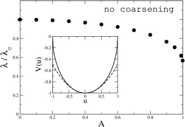
Figure 3: $\lambda(A)$ for Eq. (29), $c=0$ and $\beta=0$ (see Eq. (62)). $V(u)=-\sqrt{1-u^{2}}$ (inset) and $\lambda^{\prime}(A)<0$ (main, full circles). The dashed line is the harmonic potential $u^{2}/2$. If $c=0$, there is no coarsening whatever is $\beta$.

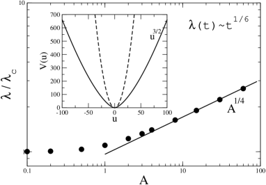
Figure 4: $\lambda(A)$ for Eq. (29), $c=\infty$ and $\beta=0$. Inset: $V(u)=\sqrt{1+m^{2}}(2m^{2}-1)/3$, with $m^{2}=(\sqrt{1+4u^{2}}-1)/2$. $V(u)\approx|u|^{3/2}$ for large $u$ and $\lambda^{\prime}(A)>0$ (main, full circles). For large amplitude, $\lambda\approx A^{1/4}$ (main, full line). The dashed line in the inset is the harmonic potential, $u^{2}/2$. If $c>0$ there is coarsening, whose law depends on $\beta$. For $\beta=0$, $\lambda(t)\approx t^{1/6}$.

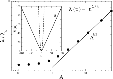
Figure 5: $\lambda(A)$ for Eq. (29), $c=\infty$ and $\beta=\infty$. Inset: $V(u)=m^{2}-(1/2)\ln(1+m^{2})$, with $m^{2}=(\sqrt{1+4u^{2}}-1)/2$. $V(u)\approx|u|$ for large $u$ and $\lambda^{\prime}(A)>0$ (main, full circles). For large amplitude, $\lambda\approx\sqrt{A}$ (main, full line). The dashed line in the inset is the harmonic potential, $u^{2}/2$. For $\beta>0$, $\lambda(t)\approx t^{1/4}$.

III.5 Discussion

In this section we have applied the results of Sec. II to find the coarsening law $\lambda(t)$ for some classes of models displaying asymptotic coarsening, that is to say having a negative phase diffusion coefficient $D$ for ‘large’ amplitude (if the amplitude $A$ has an upper limit $A_{\hbox{\footnotesize max}}$, ‘large’ means $A\to A_{\hbox{\footnotesize max}}$). In particular, in III.1-III.3 we have considered models entering into the classes

$$\partial_{t}u=B(u)+u_{xx} \Rightarrow t\sim{J(\partial_{A}\lambda)\over B(A)}$$ (65a)

$$\partial_{t}u=-\partial_{xx}[B(u)+u_{xx}] \Rightarrow t\sim{I(\partial_{A}\lambda)\over B(A)}$$ (65b)

where we have also indicated on the right the relations leading to the coarsening laws and deriving from $|D|\sim\lambda^{2}/t$, with $D$ given in Eqs. (27) and (36).

Passing from the standard GL/CH models (Sec. III.1), to models where $V(u)$ have (non quadratic) maxima at finite $u$ (Sec. III.2) and to models where $V(u)$ has no maxima at all at finite $u$ (Sec. III.3), the coarsening exponents change with continuity from $n=0$ (logarithmic coarsening) to $n=1/2$ for the nonconserved models and from $n=0$ to $n=1/4$ for the conserved models.

The conservation law, as expected, always slows down the coarsening process. Formally, this corresponds to replace the action $J$ with the quantity $I$ in the denominator of $D$. In most cases, $J$ is a constant while $I$ increases as $\lambda^{\kappa}$, with $\kappa\geq 1$: a smaller $D$ implies a lower coarsening. We remark that only in a very special case (models without uniform stable solutions and $\alpha<2$), $I/J\sim\lambda^{2}$: when this happens, the double derivative $\partial_{xx}$—which characterizes the conserved models—is equivalent (as for the coarsening law) to the factor $1/\lambda^{2}$. We stress again that this is an exception, it is not the rule.

Sec. III.4 has been devoted to a class of conserved models which are relevant for the physical problem of a growing crystal. In that case the full expression (35) for $D$ must be considered (the result is reported in Eqs. (64a-64b)). It is remarkable that for all the models we have considered, we found $n\leq 1/4$ and $n\leq 1/2$ for conserved and nonconserved models, respectively. It would be interesting to understand how general these inequalities are.

IV Swift-Hohenberg equation and coarsening

Let us start from the standard Swift-Hohenberg equation (II.2.3),

$$\partial_{t}u=-\partial_{x}^{4}u-2\partial_{x}^{2}u-(1-\delta)u-u^{3}$$ (66)

whose linear dispersion curve is $\omega(q)=\delta-(q^{2}-1)^{2}$. The phase diffusion coefficient (see Eq. (44)) is

$$D=2q{\partial_{q}(\langle u_{xx}^{2}\rangle-\langle u_{x}^{2}\rangle)\over\langle u_{x}^{2}\rangle}$$ (67)

and it should be compared to the limiting expression, valid for $\delta\to 0$,

$$D_{E}=-{1\over 2}\left[\omega^{\prime\prime}+{(\omega^{\prime})^{2}\over\omega}\right]=-{1\over 2\omega}{d\over dq}(\omega\omega^{\prime})$$ (68)

where the subscript $E$ refers to the Eckhaus instability and prime denotes derivative with respect to $q$.

Steady states satisfy the equation ${\cal L}_{SH}[u]-u^{3}=0$, where ${\cal L}_{SH}[u]$ means the linear part of the operator appearing on the right hand side of Eq. (66). In the one-harmonic approximation, $u(x)=A(q)\cos(qx)$ and the steady condition writes $\omega(q)u=u^{3}$ implying

$$\omega(q)=\langle u^{2}\rangle=1/2A^{2}(q).$$ (69)

In the same spirit we get $\langle u_{x}^{2}\rangle=q^{2}A^{2}/2=q^{2}\omega$ and $\langle u_{xx}^{2}\rangle=q^{4}A^{2}/2=q^{4}\omega$, so that $D$ reads

$$D={2\over q\omega}{d\over dq}[\omega(q^{4}-q^{2})].$$ (70)

Close to the threshold, $\delta\to 0$, $q=1+K$ (with $K\ll 1$), $\omega(q)=\delta-4K^{2}$ and $\omega^{\prime}=-8K$. Finally, we get

$$D={4\over\omega}{d\over dq}(K\omega)=D_{E}$$ (71)

so that the expression for $D$ is equal to the well known expression for $D_{E}$. It must be noted, see Eq. (69), that $A$ vanishes at $q=q_{2}$ and at $q=q_{1}$, as $\omega$ does, so that $A$ undergoes a fold singularity at the center of the band. This is imposed by symmetry, since in the vicinity of threshold the band of active modes is symmetric. In this case we are in the situation with the dispersion relation (1). The phase diffusion coefficient must also be symmetric with respect to the center, and therefore it can change sign at the fold, due to this symmetry. Thus $D$ does not have the sign of $A^{\prime}$ in this case. Nonetheless, in the vicinity of $q_{2}$ the sign of $D$ is still given by $A^{\prime}$, as shown here below. Our speculation is that the existence of a fold is likely to destroy the simple link between $D$ and $A^{\prime}$.

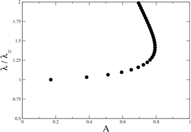
Figure 6: $\lambda(A)$ for the Swift-Hohenberg eq. (66), with $\delta=1$. The amplitude $A$ is defined as $A=[\oint dx\;u^{2}(x)/\lambda]^{1/2}$.

A meaningful expression for $D$ can be found also for finite $\delta$, close to $q_{2}=\sqrt{1+\sqrt{\delta}}$ (let us remind that $\omega(q_{1,2})=0$ and $q_{2}>q_{1}$). In this limit we get $\omega^{\prime}(q)\simeq\omega^{\prime}(q_{2})=4q_{2}-4q_{2}^{3}$ and

$$D=2(q_{2}^{3}-q_{2}){1\over\omega}{d\omega\over dq}=D_{E}$$ (72)

so that $D$ is equal to a positive quantity times $d\omega/dq$. Since $\omega(q)=A^{2}(q)/2$, the sign of $D$ is equal to the sign of $dA/dq$. This result follows from a perturbative scheme where use has been made of the fact that $u\sim\cos(qx)$. This is legitimate as long as one considers small deviations from the threshold. If $\delta$ is not small, or if $\delta=1$ we fall in the dispersion relation (3). As one deviates from $q_{2}$ towards the center of the band, higher and higher harmonics become active, and one should in general find numerically the steady state solutions in order to ascertain whether $D$ is positive or negative. In the general case, we have not been able to establish a link between $D$ and the slope of the steady state branch as done in the previous sections. Our belief, on which some evidences will be reported on in the future, is that depending on the class of equations, it is not always the slope of the steady state solution that provides direct information on the nonlinear dynamics, but somewhat a bit more abstract quantities, as we have found, for example, by investigating the KS equation, another question on which we hope to report in the near future long . Numerical solutions of the SH equation in the limit $\delta=1$ reveal a fold singularity in the branch $\lambda(A)$, as shown in Fig. 6.

V Equations with a potential

Some of the equations discussed in Sec. II.2 are derivable from a potential: it is therefore possible to define a function ${\cal F}$ which is minimized by the dynamics. This is always the case for the generalized Ginzburg-Landau equation (16), which can be written as

$$\partial_{t}u=B(u)+G(u)u_{xx}=-G(u){\delta{\cal F}\over\delta u}$$ (73)

$${\cal F}[u]=\int dx\left[\hbox{${1\over 2}$}(u_{x})^{2}-V(u)\right]$$ (74)

where $V(u)$ is the potential entering in the study of the stationary solutions, i.e. $V^{\prime}(u)=B(u)/G(u)$. If we evaluate the time derivative of ${\cal F}$ we find

$${d{\cal F}\over dt}=\int dx{\delta{\cal F}\over\delta u}u_{t}=-\int dxG(u)\left({\delta{\cal F}\over\delta u}\right)^{2}\leq 0,$$ (75)

if $G(u)>0$.

The generalized Cahn-Hilliard equation (29) can always be written as

$$\partial_{t}u=-C(u)\partial_{xx}[B(u)+G(u)u_{xx}]=C(u)\partial_{xx}[G(u){\delta{\cal F}\over\delta u}].$$ (76)

If $C(u)=G(u)$, we find

$${d{\cal F}\over dt}=-\int dx\left[\partial_{x}\left(C(u){\delta{\cal F}\over\delta u}\right)\right]^{2}\leq 0.$$ (77)

We now want to evaluate ${\cal F}$ for the steady states. The pseudo free-energy ${\cal F}$ is nothing but the integral of the Lagrangian function ${\cal L}$ for the mechanical analogy defining the stationary solutions. If $E=(u_{x})^{2}/2+V(u)$ is the ‘energy’ in the mechanical analogy and $J$ is the action,

$${\cal F}[u_{\lambda}(x)]=\ell\left({J\over\lambda}-E\right)$$ (78)

where $\ell$ is the length of the one dimensional ($1d$) interface. We have also made explicit the dependence on $\lambda$ of the stationary solutions, $u_{\lambda}(x)$. We want to determine the dependence on $\lambda$ of the pseudo free-energy,

$${d{\cal F}\over d\lambda}=\ell{d\over d\lambda}\left({J\over\lambda}-E\right)=-\ell{J\over\lambda^{2}}<0$$ (79)

where we have used that $\partial_{E}J=\lambda$. This result shows that stationary solutions with a greater wavelength always have a lower energy. Since dynamics minimizes ${\cal F}$, this result supports the idea that coarsening occurs when $\partial_{A}\lambda>0$.

If the curve $\lambda(A)$ has extrema, there are different steady states with the same value of $\lambda$: let us consider two of such states, separated by only one extremum, $\lambda(A_{1})=\lambda(A_{2})=\lambda_{0}$. We ask what state has the lower free energy. If ${\cal F}_{1,2}={\cal F}[u_{\lambda(A_{1,2})}]$ and we label the different steady states with $E=V(A)$ rather than with $A$, we get

$${{\cal F}_{2}-{\cal F}_{1}\over\ell} = {J(E_{2})-J(E_{1})\over\lambda_{0}}-(E_{2}-E_{1})$$ (80)

$$= {1\over\lambda_{0}}\int_{E_{1}}^{E_{2}}dE\lambda(E)-(E_{2}-E_{1})$$

$$= {E_{2}-E_{1}\over\lambda_{0}}(\bar{\lambda}-\lambda_{0})$$

where $\bar{\lambda}$ is the average $\lambda$ in the interval $(E_{1},E_{2})$.

Therefore, if $\lambda(A)$ has a maximum between $A_{1}$ and $A_{2}$, ${\cal F}_{1}<{\cal F}_{2}$; if $\lambda(A)$ has a minimum between $A_{1}$ and $A_{2}$, ${\cal F}_{2}<{\cal F}_{1}$. So, if two steady states have the same wavelength, the state with lower free-energy is always the state corresponding to a positive value of $\partial_{A}\lambda$.

Let us resume what we found in this section. For the gGL equations and a class of the gCH equations ($C(u)=G(u)$), there is a functional ${\cal F}$ which is minimized by the dynamics, $d{\cal F}/dt\leq 0$; if $u_{\lambda}(x)$ is a stationary solution of period $\lambda$ and we evaluate the free-energy ${\cal F}[u_{\lambda}(x)]$ for the steady branch $\lambda(A)$, then $(d/d\lambda){\cal F}[u_{\lambda}(x)]<0$, i.e. the free-energy decreases with increasing the wavelength. We are now interested to study the variation of ${\cal F}$ when the amplitude of $u_{\lambda}(x)$ is changed, keeping the period fixed.

Since $u_{\lambda}(x)$ minimizes ${\cal F}$, it is necessary to go to the second order. If $u(x)=u_{\lambda}(x)+\chi(x)$, we get

$$\Delta{\cal F} \equiv {\cal F}[u_{\lambda}(x)+\chi(x)]-{\cal F}[u_{\lambda}(x)]$$

$$= -{1\over 2}\int dx[V^{\prime\prime}(u_{\lambda})\chi^{2}(x)+\chi(x)\chi^{\prime\prime}(x)]$$

We are interested in fluctuations of the amplitude, so we take $\chi(x)=\epsilon u_{\lambda}(x)$ and we ask if $\Delta{\cal F}$ is an increasing or decreasing function of $\epsilon$:

$$\Delta{\cal F}={\epsilon^{2}\over 2}\int dx[u_{\lambda}(x)V^{\prime}(u_{\lambda})-u^{2}_{\lambda}(x)V^{\prime\prime}(u_{\lambda})]$$ (82)

What is relevant is the sign of the integral,

$${\cal Q}=\int dx[u(x)V^{\prime}(u)-u^{2}(x)V^{\prime\prime}(u)]$$ (83)

where we have removed the subscript $\lambda$ to lighten notation, keeping in mind that $u(x)$ is a stationary solution of period $\lambda$. A positive (negative) ${\cal Q}$ means that $u(x)$ is stable (unstable) against fluctuations of the amplitude: we want to relate such property to the behavior of the curve $\lambda(A)$.

Since $V(u)$ is an even function, we can define $\tilde{V}(u^{2})=V(u)$. Since $V^{\prime}=2u\tilde{V}^{\prime}$ and $V^{\prime\prime}=2V^{\prime}+4u^{2}\tilde{V}^{\prime\prime}$, we find

$${\cal Q}=-8\int dxu^{4}\tilde{V}^{\prime\prime}(u^{2}).$$ (84)

In App. A, Eqs. (90,91), we show that the sign of $\lambda^{\prime}(A)$ is related to the sign of $\tilde{V}^{\prime\prime}(u^{2})$. For convex or concave potentials $\tilde{V}(u^{2})$, we can conclude that the sign of $\Delta{\cal F}$ is equal to the sign of $\lambda^{\prime}(A)$: if $\lambda^{\prime}(A)>0$ we have phase instability (i.e. coarsening), but amplitude stability; if $\lambda^{\prime}(A)<0$ we have phase stability (i.e. constant wavelength), but amplitude instability. If the curvature of $\tilde{V}(u^{2})$ changes sign, it is no more possible to establish such a strict relation between the signes of $\Delta{\cal F}$ and $\lambda^{\prime}(A)$ for any value of $A$.

VI Summary and perspectives

VI.1 Results

The two major results of the present work are (i) the derivation of a criterion for coarsening based on the behavior of the steady state solutions. This criterion holds for several classes of nonlinear equations that are encountered in various nonequilibrium systems. The link between the steady state behavior and coarsening (which is a dynamical feature) has been made possible thanks to the phase diffusion equation. (ii) The exploitation of the phase diffusion coefficient has allowed us to derive the coarsening law. For all known examples which fall within our classes, we have captured the exact coarsening exponent. Our analysis has allowed us to make a quite general statement about the law of coarsening and on the relevant quantities that are decisive in fixing the coarsening exponent.

VI.2 Extension to higher dimension

Usually, an analytical derivation of the coarsening exponent is made for some equations where their one dimensional character is essential. While a link between the phase diffusion coefficient and the behavior of a steady state branch proves presently difficult to achieve beyond $1d$, the derivation of the phase diffusion equation can be made at arbitrary dimension. Our idea according to which $t\sim\lambda^{2}/D$ is worth testing in higher dimension. If it works, since $D$ contains only information on the periodic steady state solutions, it is sufficient to obtain these solutions to determine the coarsening law. A numerical determination of these solutions is straightforward and thus the behavior of $D$ as a function of $\lambda$ can easily be extracted. Then the coarsening law can be obtained without resorting to a time-dependent simulation.

It must be noted, however, that, for example, in two dimensions ($2d$), there are two independent phase diffusion coefficients. There are, besides bands, five Bravais lattices in $2d$ and one has first to determine the steady state solutions, which depend on the symmetries of the equation. If we take bands as a starting steady state solution, then there are two principal directions for the phase evolution: the phase diffusion along the band, and the one orthogonal to it. Usually, in the vicinity of a threshold (as in the case of Eq. (1)) diffusion along the band exhibits a zig-zag instability, while the one in the orthogonal direction is associated with the Eckhaus instability cross93 . Would only one of the two coefficients be relevant for the coarsening, or rather is there a competition between the two directions? It is clear that if the bands coalesce by keeping their steady state like symmetry (bands keep their integrity), then, for the CH equation, a logarithmic coarsening should prevail. We know, however, that the coarsening law in $2d$ is $\lambda\sim t^{1/3}$ Bray . From this, we expect that both coefficients were essential for the coarsening.

One possibility would be to make use of the idea of diffusion law ($\lambda^{2}/D\sim t$) in the anisotropic case. For example if we have two diffusion coefficients $D_{x}$ and $D_{y}$ along the two directions, by absorbing these coefficients in $x$ and $y$ coordinates in the phase equation, we arrive to $(\lambda_{x}/\sqrt{D_{x}})^{2}+(\lambda_{y}/\sqrt{D_{y}})^{2}\sim t$, where $\lambda_{x}^{2}+\lambda_{y}^{2}=\lambda^{2}$, and $D_{x}$ and $D_{y}$ depend on $\lambda_{x}$ and $\lambda_{y}$. At long time scales, it is appealing to expect that isotropy (provided the starting equation enjoys the rotational symmetry) should be, in principle, restored and $\lambda_{x}\sim\lambda_{y}\sim t^{n}$ (where $n$ is the coarsening exponent), and this should complete the extraction of the scaling with time. It is an important task for future investigations to clarify this point.

Studies on coarsening in more than $1d$ may be fairly complicated, even if a lot of progress has been done in the comprehension of phase ordering phenomena Bray . As a matter of fact, in more than $1d$ large scale temporal simulations which are performed with the aim to ascertain the coarsening law are extremely time consuming (even prohibitive in several cases). Note that, as it has been discussed in Sec. III.3, even in $1d$ the cross-over to the true asymptotic regime may prove to be very long. Thus, if our idea based on the analysis of phase diffusion should work in $2d$ (and higher dimension), it would constitute an important way for the determination of the coarsening exponent. We intend to investigate this matter on the GL equation in $2d$, and then possibly on other equations.

VI.3 More about the phase equation

The idea according to which the diffusion coefficient, even in $1d$, allows one to determine the coarsening law (although it has proven to be successful for all classes of equations discussed here) calls for additional comments. Indeed, because the phase equation $\partial_{t}\phi=D\partial_{xx}\phi$ exhibits a negative diffusion coefficient in the coarsening regime, the phase instability leads to an exponential increase of the phase in the course of time. One therefore needs to push the expansion in power series of $\epsilon$ to higher orders. It is clear that the next order should lead to the following linear term $-\kappa\partial_{xxxx}\phi$ with $\kappa>0$ in order to prevent arbitrarily small wavelength fluctuations. Nonlinear terms are also needed for the nonlinear saturation. From general considerations we expect the first nonlinear term to have the form $\partial_{x}\phi\partial_{xx}\phi$. This is dictated by the fact that the phase diffusion equation should enjoy invariance under the transformation: $x\rightarrow-x$ and $\phi\rightarrow-\phi$.

Why and how does the determination of the coarsening exponent depend solely on the inspection of $D$ is not completely understood. One possible heuristic explanation can be put forward, namely the power counting argument where at large scales only the first of these terms is decisive. It is of great importance to clarify this point further, for example by analyzing the renormalization flow of the nonlinear phase equation at large time.

VI.4 From coarsening to chaos

All the evolution equations for which our general criterion based on $\lambda(A)$ has been derived, exhibit the following dynamics: (i) they undergo perpetual coarsening, (ii) or they develop a pattern with a frozen wavelength while the amplitude increases indefinitely in the course of time. If, for example, the standard CH equation (6) is modified in the following manner

$$\partial_{t}u=-\partial_{xx}[u+\partial_{xx}u-u^{3}]+\nu u\partial_{x}u$$ (85)

where $\nu$ is a parameter (taken to be positive without restriction), we obtain a mixture between the CH and KS equations. For $\nu=0$ we recover the CH equation while for $\nu\rightarrow\infty$ we obtain the KS limit (upon an appropriate rescaling, $u\rightarrow u/\nu$). Thus for small enough values of $\nu$ a coarsening may be expected, while for large values chaos should prevail. The behavior of this solution was considered by Golovin et al. Golovin . In the spirit of our analysis we can derive the phase diffusion equation, or equivalently we can describe the stability of steady state solutions in a Floquet-Bloch picture. The branch of steady state solutions in the plane (wavelength-amplitude) is monotonous up to $\nu=0.47$, beyond which the branch exhibits a fold singularity. Numerical analysis seems to indicate that the transition from coarsening to non coarsening occurs at this value.

While it could not be proven in general that there is a link between the branch of the steady state solutions and the instability eigenvalues, it is surprising to see that coarsening stops when the branch undergoes a fold singularity. On the light of the various situations encountered here, it is appealing to speculate that whether coarsening occurs or not should be related to considerations of the behavior of the steady state solutions only. While for the class of equations like (30) the criterion could be related to the slope $\lambda(A)$, the criterion may assume a more abstract form for more general equations. It is hoped to investigate this matter further in the future.

Appendix A General considerations on $\lambda(A)$

Stationary solutions, which play the dominant role in our treatment, in most cases are determined by a Newton-type equation,

$$u_{xx}=F(u)$$ (86)

where the potential $V(u)=-\int duF(u)$ is symmetric and has a (quadratic) minimum in $u=0$. We are interested in periodic solutions $u_{0}(x)$, which correspond to oscillations of period $\lambda$ and amplitude $A$ within the potential well $V(u)$. We want to give general criteria to understand if $\lambda$ is an increasing or a decreasing function of $A$. More precisely, we are showing how is possible to determine in an easy way the behavior of $\lambda(A)$ for small and large amplitude $A$. This does not cover all possibilities, because we may find funny potentials $V(u)$ which produce an oscillating function $\lambda(A)$: in these cases a numerical analysis is necessary each time. In all the other cases, when $\lambda(A)$ has no more than one extremum, the following analysis applies. At the end of this section we are also providing an exact expression for $d\lambda/dA$, whatever is the potential $V(u)$.

It is trivial that in the harmonic approximation, $V(u)\sim u^{2}$, $\lambda$ is constant: from a dynamical point of view, this corresponds to the linear regime. The behavior at small amplitude $A$ is therefore defined by the sign of the quartic term in the potential, the third one being absent because $V(u)$ is symmetric: $V(u)\simeq u^{2}+a_{4}u^{4}$. It is easy to understand and straightforward to show (via perturbation theory Landau ) that $\partial_{A}\lambda$ has the sign opposite to $a_{4}$: $\lambda$ is an increasing (decreasing) function of $A$ if $a_{4}$ is negative (positive).

As a general rule, if the potential is steeper than a parabola, $\lambda$ decreases with increasing the amplitude; in the opposite case, $\partial_{A}\lambda>0$. Therefore, if $V(u)\approx|u|^{k}$ for large $u$, $\lambda$ increases with $A$ if $k<2$. Using the law of mechanical similarity Landau2 , i.e. scale analysis, we can find that

$$V(u)\approx|u|^{k}~{}~{}~{}{A\over\lambda^{2}}\sim A^{k-1}~{}~{}~{}~{}\lambda\sim A^{1-{k\over 2}}.$$ (87)

If $V(u)$ increases faster than a power law, e.g. exponentially, $\partial_{A}\lambda<0$ of course. The same is true if $V(u)$ diverges at finite amplitude, e.g. $V(u)=1/(1-u^{2})$, or if $V(u)$ goes to a finite value for finite amplitude, but with a diverging force, e.g. $V(u)=-\sqrt{1-u^{2}}$.

If $V(u)$ increases slower than a power law, e.g. logarithmically, or it goes to a constant for infinite $u$, or it has a maximum at finite amplitude, in all these cases $\lambda$ is an increasing function of $A$.

Now let us turn to a more rigorous analysis of $\lambda^{\prime}(A)$. The exact expression for the period $\lambda$ is

$$\lambda=2\sqrt{2}\int_{0}^{A}{du\over\sqrt{V(A)-V(u)}}.$$ (88)

If we use the formula

$${d\over dA}\int_{0}^{A}duf(u,A)$$

$$= {1\over A}\int_{0}^{A}du[A\partial_{A}f(u,A)+u\partial_{u}f(u,A)+f(u,A)]$$

we get

$${d\lambda\over dA}={\sqrt{2}\over A}\int_{0}^{A}du{R(A)-R(u)\over[V(A)-V(u)]^{3/2}}$$ (90)

where $R(u)=2V(u)-uV^{\prime}(u)$. If, following Sec. V, we introduce the function $\tilde{V}(u^{2})=V(u)$, we find that

$$R^{\prime}(u)=-4u^{3}\tilde{V}^{\prime\prime}(u^{2}).$$ (91)

Therefore, if $\tilde{V}(u^{2})$ is a convex (concave) function, $R(u)$ decreases (increases) with $u$ and $\lambda$ is a decreasing (increasing) function of the amplitude $A$.

Appendix B gCH equation: the sign of $D$

In Sec. II.2.2 we found that for the generalized Cahn-Hilliard equation, the phase diffusion coefficient has the form $D=q^{2}\partial_{q}\langle(\dots)\rangle/\tilde{D}_{2}$. In order to establish the connection between coarsening and sign of $\lambda^{\prime}(A)$, it is necessary to show that $\tilde{D}_{2}>0$. Let us recall the following:

$$\tilde{D}_{2}=-\left\langle v{\partial_{\phi}u_{0}\over C(u_{0})}\right\rangle$$ (92)

$$\partial_{\phi\phi}v={\partial_{\phi}u_{0}\over G(u_{0})}$$ (93)

$$C(u_{0})=C(-u_{0})>0~{}~{}G(u_{0})=G(-u_{0})>0$$ (94)

Since $C(u_{0})$ is an arbitrary even and positive function and $v$ does not depend on it, it is necessary to prove that $v\partial_{\phi}u_{0}\leq 0$, or, equivalently, that $v\partial_{\phi\phi}v\leq 0$. From Eq. (93), $v=v_{0}(\phi)+c_{1}+c_{2}\phi$, where $v_{0}$ is a $2\pi-$periodic function: we impose $c_{2}=0$ in order to maintain this property, while $c_{1}$ will be fixed later on.

$u_{0}(\phi)$ is the periodic, bounded trajectory of a particle moving in a symmetric potential well, with $V(u)$ being an increasing function between $u=0$ and $u=A$, the amplitude. $u_{0}(\phi)$ can be choosen as an odd function vanishing in $\phi=0,\pm\pi$, with $u_{0}(\phi)$ and $-\partial_{\phi\phi}u_{0}$ having the same sign as $\phi$. If we take the derivative of $u_{0}$, use the relation (93) and integrate $\partial_{\phi\phi}v$, we recognize that $\partial_{\phi}v$ has the same properties as $u_{0}(\phi)$. In a similar way, we can say that $\partial_{\phi\phi}v$ and $\partial_{\phi}u_{0}$ are even functions vanishing in $\pm\phi_{0}$ (the extrema of $u_{0}$ and $\partial_{\phi}v$), that $\partial_{\phi\phi}v(\phi)>0$ for $|\phi|<\phi_{0}$ and $\partial_{\phi\phi}v(\phi)<0$ outside.

Let us now integrate $\partial_{\phi}v$: $v(\phi)$ is an even function having maxima in $\pm\pi$ and a minimum in $\phi=0$. We fix the constant $c_{1}$ in such a way that $v(\phi)$ has zeros in $\pm\phi_{0}$. Therefore, since $v(\phi)<0$ for $|\phi|<\phi_{0}$ and $v(\phi)>0$ outside,

$$v\,\partial_{\phi\phi}v\leq 0,$$ (95)

as we should prove.

Appendix C The different scenarios for the ‘crystal-growth’ equation

We consider here Eq. (30)

$$\partial_{t}z=-\partial_{x}\{B(m)+G(m)\partial_{x}[C(m)\partial_{x}m]\}$$ (96)

where $m=\partial_{x}z$ and the functions $B,G,C$ are given by Eq. (62)

$$B(m)={m\over 1+m^{2}},~{}~{}G(m)={1+\beta\sqrt{1+m^{2}}\over(1+\beta)(1+m^{2})},$$

$$C(m)={1+c(1+m^{2})(1+2m^{2})\over(1+c)(1+m^{2})^{3/2}}.$$

If we perform a change of variable,

$$u=\int_{0}^{m}ds\,C(s)={m\over 1+c}{1+c(1+m^{2})\over\sqrt{1+m^{2}}}$$ (97)

we get what we named the full generalized Cahn-Hilliard equation

$$\partial_{t}u=-C(u)\partial_{xx}[B(u)+G(u)u_{xx}]$$ (98)

whose steady states correspond to the trajectories of a particle moving in the potential

$$V(u)=\int du{B(u)\over G(u)}.$$ (99)

In the general case, it is not possible to invert the function $u(m)$ so as to get an explicit form for $B(u),G(u),C(u)$ and therefore $V(u)$. However, it will be sufficient to consider the limiting expressions for $V(u)$ (small and large $u$) in order to discriminate between the possible dynamical scenarios.

Let us start by considering the case $c=0$, because analytics is simpler. The function $u(m)$ can be inverted, $m=u/\sqrt{1-u^{2}}$, showing that the limit of large amplitude $m$ corresponds for the new variable to $u\to\pm 1$. The potential $V(u)$ has the form

$$V(u)=(1+\beta)\int du{u\over\beta+\sqrt{1-u^{2}}}$$ (100)

where the parameter $\beta\geq 0$ is easily recognized to be irrelevant, so we can assume $\beta=0$ and get the approximate potential $V(u)\sim-\sqrt{1-u^{2}}$ (see Fig. 3, inset): this case had already been studied by the authors OPL , finding that $\lambda(A)$ is a decreasing function (see also the remarks in App. A). We can conclude that no coarsening appears if $c=0$.

If $c>0$, $u(m)\simeq cm^{2}/(1+c)$ for $m\gg 1$ and large amplitude now means large $u$. In this limit, $m\sim\sqrt{u}$ and $V(u)\sim(1+\beta)\sqrt{u}/(1+\beta\sqrt{u})$, so that $V(u)\sim\sqrt{u}$ for $\beta=0$ and $V(u)\sim(1+\beta)/\beta$ for $\beta>0$. In both cases—potential growing as the square root of the amplitude or going to a constant—$\lambda(A)$ is an increasing function and there will be asymptotic coarsening. The different behavior of $V(u)$ for $\beta=0$ and $\beta>0$ suggests different coarsening exponents, as are actually found.

In the previous paragraph we have considered the limit of large amplitude: now we are considering the opposite limit of small amplitude. When $m\to 0$ it is trivial to check that $u=m$, but we need the third order correction, which is easy to calculate from Eq. (97): $m\simeq u+(a/2)u^{3}$, with $a=(1-c)/(1+c)$. For small $m$,

$${B(m)\over G(m)} = {(1+\beta)m\over 1+\beta\sqrt{1+m^{2}}}\simeq{(1+\beta)m\over 1+\beta(1+m^{2}/2)}$$ (101)

$$\simeq m-{\beta\over 2(1+\beta)}m^{3}.$$

If now we pass to the variable $u$,

$$V(u) \simeq \int du\left[\left(u+{a\over 2}u^{3}\right)-{\beta\over 2(1+\beta)}u^{3}\right]$$ (102)

$$\simeq {u^{2}\over 2}+{1\over 8}\left(a-{\beta\over 2(1+\beta)}\right)u^{4},$$

we find that the behavior of the curve $\lambda(A)$ at small $A$ is fixed by the sign of the quantity $a-\beta/(2(1+\beta))$: $\lambda$ is an increasing function of $A$ (at small $A$) if that quantity is negative, i.e. if $a<\beta/(2(1+\beta))$. Using the expression $a=(1-c)/(1+c)$ we finally find that $\partial_{A}\lambda>0$ at small $A$, if $c>1/(1+2\beta)$.

References

- (1) M. C. Cross and P. C. Hohenberg, Rev. Mod. Phys. 65, 851 (1993).
- (2) M. I. Rabinovich, A. B. Ezersky, and P. D. Weidman, The dynamics of patterns (World Scientific, Singapore, 2000).
- (3) C. Misbah and A. Valance, Phys. Rev. E 49, 166 (1994), and references therein.
- (4) K. Kassner and C. Misbah, Phys. Rev. E 66, 026102 (2002).
- (5) A. A. Nepomnyashchii, Fluid Dynamics 9, 354 (1974).
- (6) Y. Kuramoto and T. Tsuzuki, Prog. Theor. Phys. 55, 356 (1976).
- (7) G.I. Sivashinsky, Acta Astron. 4, 1177 (1977).
- (8) C. Misbah and O. Pierre-Louis, Phys. Rev. E 53, 4318 (1996).
- (9) M. Sato and M. Uwaha, J. Phys. Soc. Jpn. 65, 1515 (1996).
- (10) P. Politi, G. Grenet, A. Marty, A. Ponchet, and J. Villain, Phys. Rep. 324, 271 (2000).
- (11) O. Pierre-Louis, C. Misbah, Y. Saito, Y. Krug, and P. Politi, Phys. Rev. Lett. 80, 4221 (1998).
- (12) S. Paulin, F. Gillet, O. Pierre-Louis, and C. Misbah, Phys. Rev. Lett. 86, 5538 (2001).
- (13) P. Politi and C. Misbah, Phys. Rev. Lett. 92 , 090601 (2004).
- (14) J. Kevorkian and J. D. Cole, Multiple scale and singular perturbation methods (Springer, New York, 1996).
- (15) D. Zwillinger, Handbook of differential equations (Academic Press, San Diego, 1989), p.5.
- (16) See Ref.Zwillinger , p.13.
- (17) J. S. Langer, Ann. Phys. 65, 53 (1971).
- (18) A. Torcini and P. Politi, Eur. Phys. J. B 25, 519 (2002).
- (19) A. Torcini and P. Politi (unpublished).
- (20) P. Politi and C. Misbah (unpublished).
- (21) A. J. Bray, Adv. Phys. 43, 357 (1994).
- (22) A. A. Golovin, A. A. Nepomnyashchy, S. H. Davis, and M. A. Zaks, Phys. Rev. Lett. 86, 1550 (2001).
- (23) L. D. Landau and E. M. Lifshitz, Mechanics (Pergamon Press, Oxford, 1976). See .
- (24) See Ref. Landau , .