Genetic attack on neural cryptography

Abstract

Different scaling properties for the complexity of bidirectional synchronization and unidirectional learning are essential for the security of neural cryptography. Incrementing the synaptic depth of the networks increases the synchronization time only polynomially, but the success of the geometric attack is reduced exponentially and it clearly fails in the limit of infinite synaptic depth. This method is improved by adding a genetic algorithm, which selects the fittest neural networks. The probability of a successful genetic attack is calculated for different model parameters using numerical simulations. The results show that scaling laws observed in the case of other attacks hold for the improved algorithm, too. The number of networks needed for an effective attack grows exponentially with increasing synaptic depth. In addition, finite-size effects caused by Hebbian and anti-Hebbian learning are analyzed. These learning rules converge to the random walk rule if the synaptic depth is small compared to the square root of the system size.

I Introduction

Neural cryptography Kanter et al. (2002); Kinzel and Kanter (2003) is based on the effect that two neural networks are able to synchronize by mutual learning Metzler et al. (2000); Kinzel et al. (2000). In each step of this online learning procedure they receive a common input pattern and calculate their output. Then, both neural networks use those outputs presented by their partner to adjust their own weights. So, they act as teacher and student simultaneously. Finally, this process leads to fully synchronized weight vectors.

Synchronization of neural networks is, in fact, a complex dynamical process. The weights of the networks perform random walks, which are driven by a competition of attractive and repulsive stochastic forces Ruttor et al. (2004a). Two neural networks can increase the attractive effect of their moves by cooperating with each other. But, a third network which is only trained by the other two clearly has a disadvantage, because it cannot skip some repulsive steps. Therefore, bidirectional synchronization is much faster than unidirectional learning Kinzel and Kanter (2003).

This effect can be applied to solve a cryptographic problem: Two partners $A$ and $B$ want to exchange a secret message. $A$ encrypts the message to protect the content against an opponent $E$, who is listening to the communication. But, $B$ needs $A$’s key in order to decrypt the message. Therefore, the partners have to use a cryptographic key-exchange protocol Stinson (1995) in order to generate a common secret key. This can be achieved by synchronizing two neural networks, one for $A$ and one for $B$, respectively. The attacker $E$ trains a third neural network using inputs and outputs transmitted by the partners as examples. But, on average, learning is slower than synchronization. Thus, there is only a small probability $P_{E}$ that $E$ is successful before $A$ and $B$ synchronize Kinzel and Kanter (2003).

While other cryptographic algorithms use complicated calculations based on number theory Stinson (1995), the neural key-exchange protocol only needs basic mathematical operations, namely adding and subtracting integer numbers. These can be realized efficiently in integrated circuits. Computer scientists are already working on an hardware implementation of neural cryptography Volkmer and Wallner (2004); Volkmer and Wallner (2005a, b, c).

Since the first proposal Kanter et al. (2002) of the neural key-exchange protocol, improved strategies for the attackers Klimov et al. (2003); Shacham et al. (2004) and the partners Mislovaty et al. (2003); Ruttor et al. (2004a, 2005) have been suggested and analyzed Kanter and Kinzel (2003); Kinzel and Kanter (2002, 2003); Mislovaty et al. (2002). For the geometric attack it has been found that the synaptic depth $L$ determines the security of the system: the success probability $P_{E}$ decreases exponentially with $L$, while the synchronization time $t_{\mathrm{sync}}$ increases only proportionally to $L^{2}$ Mislovaty et al. (2002); Ruttor et al. (2004b). Therefore, any desired level of security against this attack can be reached by increasing $L$.

An improved version of this method is the majority attack Shacham et al. (2004). Here a group of $M$ neural networks estimates the output of $B$’s hidden units. But, instead of updating the weights individually, $E$’s tree parity machines cooperate and adjust the weight vectors in the same way according to the majority vote. While using this method increases $P_{E}$, the scaling laws hold except for one special learning rule and random inputs Shacham et al. (2004); Ruttor et al. (2005). Therefore, neural cryptography is secure against this attack in the limit $L\rightarrow\infty$, too.

In this paper we analyze a different method for the opponent E. The genetic attack Klimov et al. (2003) is not based on optimal learning like the majority attack Shacham et al. (2004), but employs a genetic algorithm in order to select the most successful of $E$’s neural networks. First, we repeat the definition of the neural key-exchange protocol in Sec. II. We also explain why $A$ and $B$ have a clear advantage over $E$. The algorithm of the genetic attack is presented in Sec. III. Here, we show that the scaling behavior observed for the geometric attack and the majority attack also holds for the genetic attack. In Sec. IV we analyze the influence of the learning rules on synchronization and learning. Finally, the known attacks on the neural key-exchange protocol are compared regarding their efficiency. The results presented in Sec. V show that the genetic attack is less efficient than the majority attack except for some special cases.

II Neural cryptography

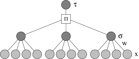
Figure 1: Tree parity machine with $K=3$ and $N=4$.

In this section we repeat the definition of the neural key-exchange protocol Kanter et al. (2002). Each partner, $A$ and $B$, uses a tree parity machine. The structure of this neural network is shown in Fig. 1. A tree parity machine consists of $K$ hidden units, which work like perceptrons. The possible input values are binary,

$$x_{ij}\in\{-1,+1\}\,,$$ (1)

and the weights are discrete numbers between $-L$ and $+L$,

$$w_{ij}\in\{-L,-L+1,\dots,L-1,L\}\,.$$ (2)

Here the index $i=1,\dots,K$ denotes the $i$th hidden unit of the tree parity machine and $j=1,\dots,N$ the elements in each vector. The output of the first layer is defined as the sign of the scalar product of inputs and weights,

$$\sigma_{i}=\mathrm{sgn}\left(\mathbf{w}_{i}\cdot\mathbf{x}_{i}\right)\,.$$ (3)

And, the total output of the tree parity machine is given by the product (parity) of the hidden units,

$$\tau=\prod_{i=1}^{K}\sigma_{i}\,.$$ (4)

At the beginning of the synchronization process $A$ and $B$ initialize the weights of their neural networks randomly. This initial state is kept secret. In each time step $t$, $K$ random input vectors $\mathbf{x}_{i}$ are generated publicly and the partners calculate the outputs $\tau^{A}$ and $\tau^{B}$ of their tree parity machines. After communicating the output bits to each other they update the weights according to one of the following learning rules:

1. Hebbian learning

   $$\mathbf{w}_{i}^{+}=\mathbf{w}_{i}+\sigma_{i}\mathbf{x}_{i}\Theta(\sigma_{i}\tau)\Theta(\tau^{A}\tau^{B})\,,$$ (5)

2. Anti-Hebbian learning

   $$\mathbf{w}_{i}^{+}=\mathbf{w}_{i}-\sigma_{i}\mathbf{x}_{i}\Theta(\sigma_{i}\tau)\Theta(\tau^{A}\tau^{B})\,,$$ (6)

3. Random walk

   $$\mathbf{w}_{i}^{+}=\mathbf{w}_{i}+\mathbf{x}_{i}\Theta(\sigma_{i}\tau)\Theta(\tau^{A}\tau^{B})\,.$$ (7)

If any component of the weight vectors moves out of the range $-L,\dots,+L$, it is replaced by the nearest boundary value, either $-L$ or $+L$.

After some time $t_{\mathrm{sync}}$ the partners have synchronized their tree parity machines, $\mathbf{w}_{i}^{A}(t_{\mathrm{sync}})=\mathbf{w}_{i}^{B}(t_{\mathrm{sync}})$, and the process is stopped. Afterwards, $A$ and $B$ can use the weight vectors as a common secret key in order to encrypt and decrypt secret messages.

We describe the process of synchronization by standard order parameters, which are also used for the analysis of online learning Engel and Van den Broeck (2001). These order parameters are

$$Q_{i}^{m} = \frac{1}{N}\mathbf{w}_{i}^{m}\cdot\mathbf{w}_{i}^{m}\,,$$ (8)

$$R_{i}^{m,n} = \frac{1}{N}\mathbf{w}_{i}^{m}\cdot\mathbf{w}_{i}^{n}\,,$$ (9)

where the indices $m,n\in\{A,B,E\}$ denote $A$’s, $B$’s or $E$’s tree parity machine, respectively. The level of synchronization between two corresponding hidden units is defined by the (normalized) overlap,

$$\rho_{i}^{m,n}=\frac{\mathbf{w}_{i}^{m}\cdot\mathbf{w}_{i}^{n}}{\sqrt{\mathbf{w}_{i}^{m}\cdot\mathbf{w}_{i}^{m}}\sqrt{\mathbf{w}_{i}^{n}\cdot\mathbf{w}_{i}^{n}}}=\frac{R_{i}^{m,n}}{\sqrt{Q_{i}^{m}Q_{i}^{n}}}\,.$$ (10)

Uncorrelated weight vectors have $\rho=0$, while the maximum value $\rho=1$ is reached for full synchronization.

The overlap between two corresponding hidden units increases if the weights of both neural networks are updated in the same way. Coordinated moves, which occur for identical $\sigma_{i}$, have an attractive effect.

Changing the weights in only one hidden unit decreases the overlap on average. These repulsive steps can only occur if the two output values $\sigma_{i}$ are different. The probability for this event is given by the well-known generalization error of the perceptron, Engel and Van den Broeck (2001)

$$\epsilon_{i}=\frac{1}{\pi}\arccos\rho_{i}\,,$$ (11)

which itself is a function of the overlap $\rho_{i}$ between the hidden units. For an attacker who simply trains a third tree parity machine using the examples generated by $A$ and $B$, repulsive steps occur with probability $P_{r}^{E}=\epsilon_{i}$, because $E$ cannot influence the process of synchronization.

In contrast, $A$ and $B$ communicate with each other and are able to interact. If they disagree on the total output, there is at least one hidden unit with $\sigma_{i}^{A}\neq\sigma_{i}^{B}$. As an update would have a repulsive effect, the partners just do not change the weights. In doing so, $A$ and $B$ reduce the probability of repulsive steps in their hidden units. For $K=3$ and identical generalization error, $\epsilon_{i}=\epsilon$, we find Ruttor et al. (2004a)

$$P_{r}^{B}=\frac{2(1-\epsilon)\epsilon^{2}}{(1-\epsilon)^{3}+3(1-\epsilon)\epsilon^{2}}\leq\epsilon=P_{r}^{E}\,.$$ (12)

Therefore, the partners have a clear advantage over an attacker using only simple learning.

But, $E$ can use a more advanced method called geometric attack. As before, she trains a third tree parity machine, which has the same structure as $A$’s and $B$’s. In each step $\tau^{E}$ is calculated and compared to $\tau^{B}$. As long as these output values are identical, $E$ can apply the learning rule in the same manner as $B$. But, if $\tau^{E}\neq\tau^{B}$, the attacker has to correct this deviation before updating the weights.

For this purpose $E$ uses the local field

$$h_{i}=\frac{1}{\sqrt{N}}\mathbf{w}_{i}\cdot\mathbf{x}_{i}$$ (13)

of her hidden units as additional information. Then, the probability of $\sigma_{i}^{B}\neq\sigma_{i}^{E}$ is given by the prediction error of the perceptron Ein-Dor and Kanter (1999)

$$\epsilon_{i}(\rho_{i},h_{i})=\frac{1}{2}\left[1-\mathrm{erf}\left(\frac{\rho_{i}}{\sqrt{2(1-\rho_{i}^{2})}}\frac{|h_{i}|}{\sqrt{Q_{i}}}\right)\right]\,.$$ (14)

If the local field $h_{i}$ is zero, the neural network has no information about the input vector $\mathbf{x}_{i}$, because it is perpendicular to the weight vector $\mathbf{w}_{i}$. In this case the prediction error reaches its global maximum of $\epsilon_{i}(\rho_{i},0)=1/2$.

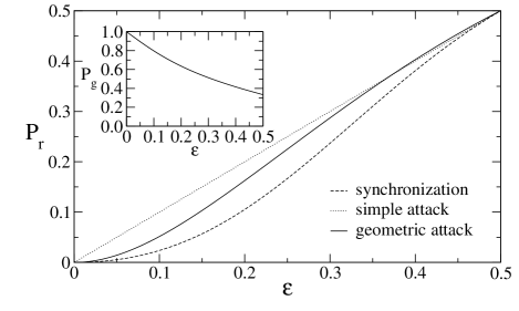
Figure 2: Probability $P_{r}$ of repulsive steps as a function of the generalization error $\epsilon$. The inset shows the probability $P_{g}$ for a successful geometric correction.

The prediction error $\epsilon_{i}(\rho_{i},h_{i})$ is a strictly monotonic decreasing function of $|h_{i}|$. Therefore, the attacker searches the hidden unit with the lowest value of the absolute local field $|h_{i}^{E}|$ and flips the sign of $\sigma_{i}^{E}$. This results in $\tau^{E}=\tau^{B}$ and the learning rule can be applied. But, the geometric attack does not always find the correct hidden unit which caused the deviation of the total output bits. If $\sigma_{i}^{E}\neq\sigma_{i}^{B}$ in the $i$th hidden unit and $\sigma_{j}^{E}=\sigma_{j}^{B}$ in all other hidden units, $E$ flips the sign of $\sigma_{i}^{E}$ with probability

$$P_{g} = \int_{0}^{\infty}\prod_{j\neq i}\left(\int_{h_{i}}^{\infty}\sqrt{\frac{2\pi}{Q_{j}}}\frac{1-\epsilon_{j}(\rho_{j},h_{j})}{\pi-\arccos\rho_{j}}e^{-\frac{h_{j}^{2}}{2Q_{j}}}\mathrm{d}h_{j}\right)$$ (15)

$$\times \sqrt{\frac{2\pi}{Q_{i}}}\frac{\epsilon_{i}(\rho_{i},h_{i})}{\arccos\rho_{i}}e^{-\frac{h_{i}^{2}}{2Q_{i}}}\mathrm{d}h_{i}\,.$$

Thus, the geometric attacker avoids some repulsive steps, although they still occur more frequently than in the partners’ tree parity machines.

In the case of identical generalization error $\epsilon_{i}=\epsilon$ and $K=3$, we find that the probability of repulsive steps,

$$P_{r}^{E}=2(1-P_{g})(1-\epsilon)^{2}\epsilon+2(1-\epsilon)\epsilon^{2}+\frac{2}{3}\epsilon^{3}\,,$$ (16)

is higher than $P_{r}^{B}$, but lower than $P_{r}^{E}=\epsilon$ for simple learning. This result is clearly visible in Fig. 2. That is why learning by listening is slower than mutual learning, even for advanced algorithms. This effect makes neural cryptography feasible and prevents successful attacks in the limit $L\rightarrow\infty$.

Recently, it has been discovered that the security of the neural key-exchange protocol can be improved by using queries instead of random inputs Kinzel and Rujan (1990); Ruttor et al. (2005). The partners ask questions to each other which depend on their own weight vectors $\mathbf{w}_{i}$ and an additional public parameter $H$. In odd (even) steps $A$ ($B$) generates $K$ input vectors $\mathbf{x}_{i}$ with $h_{i}^{A}\approx\pm H$ ($h_{i}^{B}\approx\pm H$). So, the absolute value of the local field $h_{i}$ is given by $H$, while its sign $\sigma_{i}$ is chosen randomly.

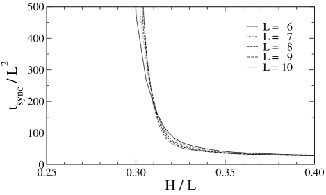
Figure 3: Synchronization time $t_{\mathrm{sync}}$ as a function of $H$ for $K=3$, $N=1000$, random walk learning rule, and different values of $L$, averaged over $10\,000$ simulations.

Queries change the relation between the overlap and the frequency $P_{r}$ of repulsive steps. The probability of different outputs $\sigma_{i}$ in corresponding hidden units is now given by Eq. (14) instead of Eq. (11), because the absolute local field in $A$’s or $B$’s hidden units is known. Consequently, the partners can optimize complexity and security of the neural key-exchange protocol by adjusting $H$ and $L$ suitably Ruttor et al. (2005).

As shown in Fig. 3, a minimum value of $H$ is needed in order to achieve synchronization in a reasonable number of steps. If $H>\alpha_{c}L$, $t_{\mathrm{sync}}$ increases proportional to $L^{2}\ln N$, but for $H<\alpha_{c}L$ it diverges Ruttor et al. (2005, 2004b). In the case of the random walk learning rule we estimate $\alpha_{c}\approx 0.31$ by using the extrapolation method described in Ruttor et al. (2005).

III Genetic Attack

Figure 4: Success probability $P_{E}$ of the genetic attack for $K=3$, $N=1000$, random walk learning rule, and $M=4096$. Symbols represent results obtained from $1000$ simulations, and the lines show a fit with Eq. (17).

For the genetic attack Klimov et al. (2003) the opponent starts with only one tree parity machine, but she can use up to $M$ neural networks. As before $E$ calculates the output of her networks in each step. Afterwards the following genetic algorithm is applied:

1. If $\tau^{A}=\tau^{B}$ and $E$ has at most $M/2^{K-1}$ tree parity machines, she determines all $2^{K-1}$ internal representations $(\sigma_{1}^{E},\dots,\sigma_{K}^{E})$ which reproduce the output $\tau^{A}$. Then, these are used to update the weights in $E$’s neural networks according to the learning rule, so that $2^{K-1}$ variants of each tree parity machine are generated.

2. But, if $E$ already has more than $M/2^{K-1}$ neural networks, the mutation step described above is not possible. Instead of that the attacker discards all tree parity machines which predicted less than $U$ outputs $\tau^{A}$ in the last $V$ learning steps, with $\tau^{A}=\tau^{B}$, successfully. In our simulations we use a limit of $U=10$ and a history of $V=20$ as default values. Additionally, at least 20 neural networks are kept in such a selection step.

3. In the case of $\tau^{A}\neq\tau^{B}$ the attacker’s networks remain unchanged, because $A$ and $B$ do not update the weights in their tree parity machines.

The attack is considered successful if at least one of $E$’s neural networks has synchronized $98\%$ of the weights before the end of the key exchange. We use this relaxed criterion in order to decrease the fluctuations of $P_{E}$ Mislovaty et al. (2002).

The success probability of the genetic attack strongly depends on the value of the parameter $H$. This effect is clearly visible in Fig. 4. In order to determine $P_{E}$ as a function of $H$, a Fermi-Dirac distribution

$$P_{E}=\frac{1}{1+\exp[-\beta(H-\mu)]}$$ (17)

with two parameters $\beta$ and $\mu$ can be used as a fitting model. This equation is also valid for the geometric attack and the majority attack Ruttor et al. (2005).

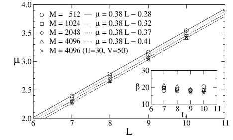
Figure 5: Parameters $\mu$ and $\beta$ as a function of the synaptic depth $L$. Symbols denote results of fitting simulation data for different $M$ with Eq. (17) and the lines were calculated using the model given in Eq. (19).

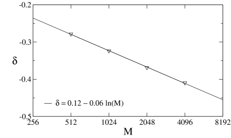
Figure 6: Offset $\delta$ as a function of the number of attackers $M$, for $K=3$, $N=1000$, and the random walk learning rule. Symbols and the line were obtained by a fit with Eq. (19).

Figure 5 shows the results of the fits using Eq. (17). While $\beta$ is nearly independent of $L$ and $M$, $\mu$ increases linearly with the synaptic depth,

$$\mu=\alpha_{s}L+\delta\,.$$ (18)

Obviously, the attacker can change the offset $\delta$, but not $\alpha_{s}$, by using more resources. As shown in Fig. 6 $E$ needs to double $M$ in order to decrease $\delta$ by a fixed amount $\gamma\ln 2$. Thus, $\mu$ is a linear function of both $L$ and $\ln M$,

$$\mu=\alpha_{s}L-\gamma\ln M+\mu_{0}\,.$$ (19)

Substituting Eq. (19) into Eq. (17) leads to

$$P_{E}=\frac{1}{1+\exp[\beta(\mu_{0}-\gamma\ln M)]\exp[\beta(\alpha_{s}-\alpha)L]}$$ (20)

for the success probability of the genetic attack as a function of $\alpha=H/L$, the synaptic depth $L$, and the maximal number of attackers $M$.

From these results we can deduce the scaling of $P_{E}$ with regard to $L$ and $M$. For large values of the synaptic depth the asymptotic behavior is given by

$$P_{E}\sim e^{-\beta(\mu_{0}-\gamma\ln M)}e^{-\beta(\alpha_{s}-\alpha)L}$$ (21)

as long as $\alpha<\alpha_{s}$.

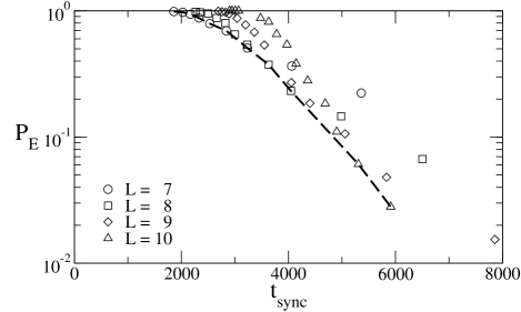
Figure 7: Success probability of the genetic attack as a function of the synchronization time for $K=3$, $N=1000$, random walk learning rule, $M=4096$ and different values of $L$. The dashed line shows the envelope of this set of curves.

This equation shows that that the partners have a great advantage over an attacker. If $A$ and $B$ increase $L$, the success probability drops exponentially,

$$P_{E}\propto e^{-\beta(\alpha_{s}-\alpha)L}\,,$$ (22)

while the complexity of the synchronization rises only polynomially. This is clearly visible if one looks at the function $P_{E}(\langle t_{\mathrm{sync}}\rangle)$, which is shown in Fig. 7. Due to the offset $\delta$ in Eq. (18) the attacker is successful for small values of $L$. But, for larger synaptic depth optimal security is reached for values of $H$ and $L$, which lie on the envelope of $P_{E}(\langle t_{\mathrm{sync}}\rangle)$. This curve is approximately given by $H=\alpha_{c}L$, as this condition maximizes $\alpha_{s}-\alpha$ while synchronization is still possible Ruttor et al. (2005).

In contrast, the attacker has to increase the number of her tree parity machines exponentially,

$$M\propto e^{[(\alpha_{s}-\alpha)/\gamma]L}\,,$$ (23)

in order to compensate a change of $L$ and maintain a constant success probability $P_{E}$. But, this is usually not possible due to limited computer power.

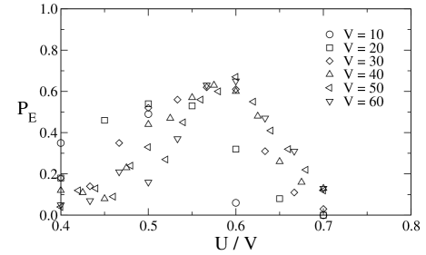
Figure 8: Success probability of the genetic attack for $K=3$, $L=7$, $N=1000$, random walk learning rule, $M=4096$, and $H=2.28$. These results were obtained by averaging over $100$ simulations.

Alternatively, the attacker could try to optimize the other two parameters of the genetic attack. As shown in Fig. 8, $E$ obtains the best result if she uses $U=30$, $V=50$ instead of $U=10$, $V=20$. Figure 5 shows that this modification leads to a lower value of $\beta$, but does not influence $\mu(L)$. Therefore, $E$ gains little, as the scaling relation (23) is not affected. That is why $A$ and $B$ can easily reach an arbitrary level of security.

IV Learning rules

Beside the random walk learning rule (7) used so far, there are two other suitable algorithms for updating the weights: the Hebbian learning rule (5) and the anti-Hebbian learning rule (6). The only difference between these three rules is whether and how the output $\sigma_{i}$ of the hidden unit is included in the update step. But, this causes some effects which we discuss in this section.

In the case of the Hebbian rule $A$’s and $B$’s tree parity learn their own output. Therefore, the direction in which the weight $w_{ij}$ moves is determined by the product $\sigma_{i}x_{ij}$. But, as the output of a hidden units is a function of all input values, there are correlations between $x_{ij}$ and $\sigma_{i}$. That is why the probability distribution of $\sigma_{i}x_{ij}$ is not uniformly distributed in the case of random inputs, but depends on the corresponding weight $w_{ij}$,

$$P(\sigma_{i}x_{ij}=1)=\frac{1}{2}\left[1+\mathrm{erf}\left(\frac{w_{ij}}{\sqrt{NQ_{i}-w_{ij}^{2}}}\right)\right]\,.$$ (24)

According to this equation, $\sigma_{i}x_{ij}=\mathrm{sgn}(w_{ij})$ occurs more often than $\sigma_{i}x_{ij}=-\mathrm{sgn}(w_{ij})$. Thus, the Hebbian learning rule (5) pushes the weights towards the boundaries at $-L$ and $+L$.

In order to quantify this effect we calculate the stationary probability distribution of the weights. Using Eq. (24) for the transition probabilities leads to

$$P(w_{ij}=w)=p_{0}\prod_{m=1}^{|w|}\frac{1+\mathrm{erf}\left(\frac{m-1}{\sqrt{NQ_{i}-(m-1)^{2}}}\right)}{1-\mathrm{erf}\left(\frac{m}{\sqrt{NQ_{i}-m^{2}}}\right)}\,,$$ (25)

whereas the normalization constant $p_{0}$ is given by

$$p_{0}=\left(\sum_{w=-L}^{L}\prod_{m=1}^{|w|}\frac{1+\mathrm{erf}\left(\frac{m-1}{\sqrt{NQ_{i}-(m-1)^{2}}}\right)}{1-\mathrm{erf}\left(\frac{m}{\sqrt{NQ_{i}-m^{2}}}\right)}\right)^{-1}\,.$$ (26)

In the limit $N\rightarrow\infty$ the argument of the error function vanishes and the weights are uniformly distributed. In this case the synchronization process does not change the initial length

$$\sqrt{Q_{i}(t=0)}=\sqrt{\frac{L(L+1)}{3}}$$ (27)

of the weight vector.

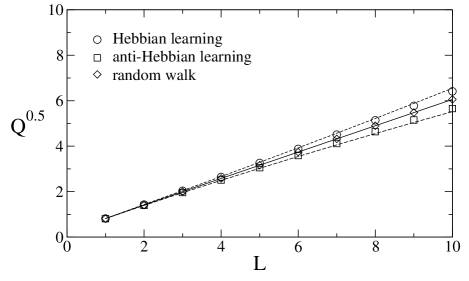
Figure 9: Length of the weight vectors in the steady state for $K=3$ and $N=1000$. Symbols denote results averaged over $1000$ simulations and lines show the first-order approximation given in Eq. (29) and Eq. (31).

But, for finite $N$ the probability distribution (25) itself depends on the order parameter $Q_{i}$. Therefore, the expectation value of $Q_{i}$ is the solution of the following equation:

$$Q_{i}=\sum_{w=-L}^{L}w^{2}P(w_{ij}=w)\,.$$ (28)

By expanding Eq. (28) in terms of $N^{-1/2}$ we obtain

$$Q_{i} = \frac{L(L+1)}{3}$$ (29)

$$+ \frac{8L^{4}+16L^{3}-10L^{2}-18L+9}{15\sqrt{3\pi L(L+1)}}\frac{1}{\sqrt{N}}$$

$$+ \mathrm{O}\left(\frac{L^{4}}{N}\right)$$

as a first-order approximation of $Q_{i}$ for large system sizes. In the case of $1\ll L\ll\sqrt{N}$ the asymptotic behavior of this order parameter is given by

$$Q_{i}\sim\frac{L(L+1)}{3}\left(1+\frac{8}{5\sqrt{3\pi}}\frac{L}{\sqrt{N}}\right)\,.$$ (30)

Obviously, the application of the Hebbian learning rule increases the length of the weight vectors $\mathbf{w}_{i}$ until a steady state is reached. Additionally, the changed probability distribution of the weights affects the synchronization process and the success of attacks. That is why one encounters finite-size effects if $L/\sqrt{N}$ is large Mislovaty et al. (2002).

In the case of the anti-Hebbian rule $A$’s and $B$’s tree parity machines learn the opposite of their own outputs. Therefore, the weights are pulled away from the boundaries, so that

$$Q_{i} = \frac{L(L+1)}{3}$$ (31)

$$- \frac{8L^{4}+16L^{3}-10L^{2}-18L+9}{15\sqrt{3\pi L(L+1)}}\frac{1}{\sqrt{N}}$$

$$+ \mathrm{O}\left(\frac{L^{4}}{N}\right)$$

$$\sim \frac{L(L+1)}{3}\left(1-\frac{8}{5\sqrt{3\pi}}\frac{L}{\sqrt{N}}\right)$$ (32)

for $1\ll L\ll\sqrt{N}$. Here, the length of the weight vectors $\mathbf{w}_{i}$ is decreased.

In contrast, the random walk learning rule always uses a fixed set output. Here, the weights stay uniformly distributed, because only the random input values $x_{ij}$ determine the direction of the movements. In this case the length of the weight vectors is given by Eq. (27).

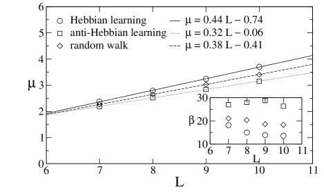
Figure 10: Parameter $\mu$ and $\beta$ as a function of $L$ for the genetic attack with $K=3$, $N=1000$, and $M=4096$. The symbols represent results from $1000$ simulations and the lines show a fit using the model given in Eq. (19).

Figure 9 shows that the theoretical predictions are in good quantitative agreement with simulation results as long as $L^{2}$ is small compared to the system size $N$. The deviations for large $L$ are caused by higher-order terms which are ignored in Eq. (29) and Eq. (31).

The choice of the learning rule affects synchronization with random inputs as well as with queries. As the prediction error (14) is a function of $h_{i}/\sqrt{Q_{i}}$, this ratio instead of just the local field determines the behavior of the system. That is why there are different values of $\alpha_{c}$ and $\alpha_{s}$ for each learning rule, which is shown in Fig. 10 and Fig. 11.

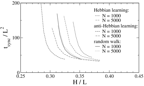
Figure 11: Synchronization time $t_{\mathrm{sync}}$ as a function of $H$ for $K=3$, $L=7$, averaged over $100$ simulations.

In the limit $N\rightarrow\infty$, however, a system using Hebbian or anti-Hebbian learning exhibits the same dynamics as observed in the case of the random walk rule for all system sizes. This is clearly visible in Fig. 11. Consequently, one can determine the properties of neural cryptography in the limit $N\rightarrow\infty$ without actually analyzing very large systems. It is sufficient to use the random walk learning rule and moderate values of $N$ in simulations.

V Security

In order to assess the security of the neural key-exchange protocol one has to consider all known attacks. Therefore, we compare the efficiency of several methods here.

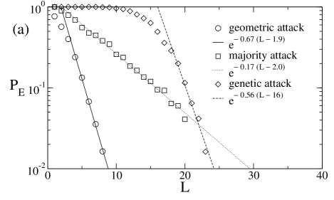
Figure 12: Success probability $P_{E}$ of the geometric attack with $M=1$, the majority attack with $M=100$, and the genetic attack with $M=4096$, for $K=3$, $N=1000$, and the random walk learning rule. Symbols represent results averaged over $1000$ simulations, in part (a) for random inputs and in part (b) for queries with $H=0.32L$. The lines were obtained by fitting with Eq. (33).

Figure 12 shows that the success probability $P_{E}$ drops exponentially with increasing synaptic depth $L$,

$$P_{E}\sim e^{-y(L-L_{0})}\,,$$ (33)

as long as $L>L_{0}$. While this scaling behavior is the same for all attacks, the constants $y$ and $L_{0}$ are different for each method.

The geometric attack is the simplest method considered here. $E$ only needs one tree parity machine, but the success probability $P_{E}$ is lower than for the advanced methods. As the exponent $y$ is large, the two partners can easily secure the neural key-exchange protocol by increasing the synaptic depth Mislovaty et al. (2002).

In the case of the majority attack $P_{E}$ is higher, because the cooperation between $E$’s tree parity machines reduces the coefficient $y$. $A$ and $B$ have to compensate this by further stepping up $L$. In contrast, the genetic attack increases $L_{0}$, while $y$ does not change significantly compared to the geometric attack. Therefore, the genetic algorithm is better only if $L$ is not too large. Otherwise $E$ gains most by using the majority attack.

As shown in Fig. 12 the partners can improve the security of the key-exchange protocol against all three attacks by using queries. However, the majority attack remains the most efficient of $E$’s methods.

We note that these results are based on numerical extrapolations of the success probability $P_{E}$. While analytical evidence for the complexity of a successful attack would be desirable, it is not available yet in the case of the nondeterministic methods with $P_{E}<1$ discussed above. But there are only two successful deterministic algorithms for $E$ known at present: a brute-force attack or a genetic attack with $M=2^{(K-1)t_{\mathrm{sync}}}$ networks. The complexity of these attacks clearly grows exponentially with increasing $L$. Therefore, breaking the security of neural cryptography belongs to the complexity class $NP$ (nondeterministic polynomial time), but we cannot prove that it is not in $P$ (polynomial time). This situation is similar to that of other cryptographic protocols, e.g., the Diffie-Hellman key exchange Stinson (1995).

VI Conclusions

The security of cryptographic algorithms is usually based on different scaling laws regarding the computational complexity for users and attackers. By changing some parameter one can increase the cost of a successful attack exponentially, while the effort for the users increments only polynomially. For conventional cryptographic systems this parameter is the length of the key. In the case of neural cryptography it is the synaptic depth $L$ of the neural networks.

As the neural key-exchange protocol uses tree parity machines, an attacker faces the challenge to guess the internal representation of these networks correctly. Learning alone is not sufficient to solve this problem. Otherwise the scaling laws hold and the partners can achieve any desired level of security by increasing $L$.

We have analyzed an attack, which combines learning with a genetic algorithm. We have found that this method is very successful as long as $L$ is small. But, attackers have to increase the number of their neural networks exponentially in order to compensate higher values of $L$. That is why neural cryptography is secure against the genetic attack as well.

This method achieves the best success probability of all known methods only if the synaptic depth $L$ is not too large. For higher values of $L$ the attacker gains more by using the majority attack. But, both methods are unable to break the security of the neural key-exchange protocol in the limit $L\rightarrow\infty$.

Additionally, we have studied the influence of different learning rules on the neural key-exchange protocol. Hebbian and anti-Hebbian learning change the order parameter $Q$, which is related to the length of the weight vectors. If the system size $N$ is small compared to $L^{2}$, this causes finite-size effects. But, in the limit $L/\sqrt{N}\rightarrow 0$ the behavior of all learning rules converges to that of the random walk rule.

Based on our results, we conclude that the neural key-exchange protocol is secure against all attacks known up to now. But—similar to other cryptographic algorithms—there is always a possibility that a clever method may be found which destroys the security of neural cryptography completely.

References

- Kanter et al. (2002) I. Kanter, W. Kinzel, and E. Kanter, Europhys. Lett. 57, 141 (2002), eprint cond-mat/0202112.
- Kinzel and Kanter (2003) W. Kinzel and I. Kanter, J. Phys. A 36, 11173 (2003).
- Metzler et al. (2000) R. Metzler, W. Kinzel, and I. Kanter, Phys. Rev. E 62, 2555 (2000), eprint cond-mat/0003051.
- Kinzel et al. (2000) W. Kinzel, R. Metzler, and I. Kanter, J. Phys. A 33, L141 (2000), eprint cond-mat/9906058.
- Ruttor et al. (2004a) A. Ruttor, W. Kinzel, L. Shacham, and I. Kanter, Phys. Rev. E 69, 046110 (2004a), eprint cond-mat/0311607.
- Stinson (1995) D. R. Stinson, Cryptography: Theory and Practice (CRC Press, Boca Raton, FL, 1995).
- Volkmer and Wallner (2004) M. Volkmer and S. Wallner, in Proceedings of the 2nd German Workshop on Mobile Ad-hoc Networks, WMAN 2004, edited by P. Dadam and M. Reichert (Bonner Köllen Verlag, Ulm, 2004), vol. P-50 of Lecture Notes in Informatics (LNI), pp. 128–137.
- Volkmer and Wallner (2005a) M. Volkmer and S. Wallner, in Proceedings of the 1st International Workshop on Secure and Ubiquitous Networks, SUN’05 (IEEE Computer Society, Copenhagen, 2005a), pp. 241–245.
- Volkmer and Wallner (2005b) M. Volkmer and S. Wallner, in ECRYPT (European Network of Excellence for Cryptology) Workshop on RFID and Lightweight Crypto (Graz University of Technology, Graz, 2005b), pp. 102–113.
- Volkmer and Wallner (2005c) M. Volkmer and S. Wallner, IEEE Trans. Comput. 54, 421 (2005c), eprint cs.CR/0408046.
- Klimov et al. (2003) A. Klimov, A. Mityaguine, and A. Shamir, in Advances in Cryptology—ASIACRYPT 2002, edited by Y. Zheng (Springer, Heidelberg, 2003), p. 288.
- Shacham et al. (2004) L. N. Shacham, E. Klein, R. Mislovaty, I. Kanter, and W. Kinzel, Phys. Rev. E 69, 066137 (2004), eprint cond-mat/0312068.
- Mislovaty et al. (2003) R. Mislovaty, E. Klein, I. Kanter, and W. Kinzel, Phys. Rev. Lett. 91, 118701 (2003), eprint cond-mat/0302097.
- Ruttor et al. (2005) A. Ruttor, W. Kinzel, and I. Kanter, J. Stat. Mech. 2005, P01009 (2005), eprint cond-mat/0411374.
- Kanter and Kinzel (2003) I. Kanter and W. Kinzel, in Proceedings of the XXII Solvay Conference on Physics on the Physics of Communication, edited by I. Antoniou, V. A. Sadovnichy, and H. Wather (World Scientific, Singapore, 2003), p. 631.
- Kinzel and Kanter (2002) W. Kinzel and I. Kanter, in Advances in Solid State Physics, edited by B. Kramer (Springer, Berlin, 2002), vol. 42, pp. 383–391, eprint cond-mat/0203011.
- Mislovaty et al. (2002) R. Mislovaty, Y. Perchenok, I. Kanter, and W. Kinzel, Phys. Rev. E 66, 066102 (2002), eprint cond-mat/0206213.
- Ruttor et al. (2004b) A. Ruttor, G. Reents, and W. Kinzel, J. Phys. A 37, 8609 (2004b), eprint cond-mat/0405369.
- Engel and Van den Broeck (2001) A. Engel and C. Van den Broeck, Statistical Mechanics of Learning (Cambridge University Press, Cambridge, 2001).
- Ein-Dor and Kanter (1999) L. Ein-Dor and I. Kanter, Phys. Rev. E 60, 799 (1999).
- Kinzel and Rujan (1990) W. Kinzel and P. Rujan, Europhys. Lett. 13, 473 (1990).