A phenomenological theory giving the full statistics of the position of fluctuating pulled fronts

Abstract

We propose a phenomenological description for the effect of a weak noise on the position of a front described by the Fisher-Kolmogorov-Petrovsky-Piscounov equation or any other travelling wave equation in the same class. Our scenario is based on four hypotheses on the relevant mechanism for the diffusion of the front. Our parameter-free analytical predictions for the velocity of the front, its diffusion constant and higher cumulants of its position agree with numerical simulations.

I Introduction

The Fisher Kolmogorov-Petrovsky-Piscounov (FKPP) equation Fisher (1937)

$$\partial_{t}h=\partial_{x}^{2}h+h-h^{2},$$ (1)

describes how a stable phase ($h(x,t)=1$ for $x\to-\infty$) invades an unstable phase ($h(x,t)=0$ for $x\to+\infty$) and how the front between these two phases builds up and travels van Saarloos (2003). This equation was first introduced in a problem of genetics, but equations similar to (1) appear in much broader contexts like reaction-diffusion problemsPechenik and Levine (1999); Doering et al. (2003), optimizationMajumdar and Krapivsky (2003), disordered systemsDerrida and Spohn (1988); Carpentier and Le Doussal (2000) and even particle physicsMunier and Peschanski (2003); Balitsky (1996); Marquet et al. (2005). A remarkable example is the problem of the high energy scattering of a projectile consisting of a small color dipole on a target in the framework of quantum chromodynamics (QCD): in Ref. Munier and Peschanski (2003) it was recognized that the Balitsky-Kovchegov (BK) equation Balitsky (1996), a mean field equation for high energy scattering in QCD, is in the same class as the FKPP equation with $h$ being the scattering amplitude, $t$ the rapidity of the scattering and $x$ the logarithm of the inverse projectile size.

It is well knownAronson and Weinberger (1975); van Saarloos (2003) that equations like (1) have a family of travelling wave solution of the form $h(x,t)=h(z)$ with $z=x-vt$. There is a relation between the exponential decay of each solution ($h(z)\sim\exp(-\gamma z)$ for large $z$) and its velocity: $v=v(\gamma)$. For example, $v(\gamma)=\gamma+1/\gamma$ for the FKPP equation (1). Other front equations would give different expressions of $v(\gamma)$. See, for example, section IV, or Refs. Brunet and Derrida (1997); Enberg et al. (2005).

If one starts with a steep enough initial condition, the front converges to the travelling wave with the minimal velocity. Therefore

$$v_{\text{deterministic}} =\min_{\gamma}v(\gamma)=v(\gamma_{0})\text{\quad where\quad}v^{\prime}(\gamma_{0})=0,$$

$$h_{\text{deterministic}}(z) \approx Aze^{-\gamma_{0}z}.$$ (2)

(The multiplicative factor $z$ in $h_{\text{deterministic}}$ is present only for this slowest moving solution.)

There is a large class (the FKPP class) of equations describing the propagation of a front into an unstable state which select the minimal velocity, as described by (2). (There exist also equations, called “pushed” or “type II” for which the velocity selected by the front is not the slowest one. The properties of these fronts are quite differentKessler et al. (1998); van Saarloos (2003) from the properties of (1), and we will not consider them in the present paper.)

Deterministic front equations such as (1) usually occur as the limit of a stochastic reaction-diffusion model Panja (2003) when the number of particles (or bacterias, or reactants) involved becomes infinite. In a physical situation, all numbers remain finite and a small noise term should be added to (1) to represent the fluctuations at the microscopic scale. One might write, for instanceMueller and Sowers (1995),

$$\partial_{t}h=\partial_{x}^{2}h+h-h^{2}+\sqrt{h(1-h)/N}\ \eta(x,t),$$ (3)

where $\eta(x,t)$ is a normalized Gaussian white noise and $N$ is the number of particles involved.

The effect of such a noise is to make the shape of the travelling wave fluctuate in timeDoering et al. (2003). It affects also its velocity and makes the front diffuseBrunet and Derrida (1999); Panja (2003); van Saarloos (2003).

For a chemical problem, $N$ might be of the order of the Avogadro number and one could think that such a small noise term should give small corrections, of order $1/\sqrt{N}$, to the shape and position of the front. However, because the front motion is extremely sensitive to small fluctuations in the region where $h\simeq 1/N$, this is not the case. In presence of noise as in (3), the front has an exponential decay if $h(x,t)\gg 1/N$, but it vanishes much faster than this exponential in the region where $h(x,t)$ is of order $1/N$ Doering et al. (2003). (This is obvious in a particle model, as there cannot be less than one particle at a given place.) As an approximation to understand the effect of the microscopic stochastic details of the system, it has been suggested to replace the noise term by a deterministic cutoff which makes the front vanish very quickly when $h\simeq 1/N$ Brunet and Derrida (1997). For instance, for the FKPP equation (1), one way of introducing the cutoff is

$$\begin{gathered}\partial_{t}h=\partial_{x}^{2}h+\big{(}h-h^{2}\big{)}a(Nh),\\ \text{with $a(r)=1$ for $r>1$ and $a(r)\to 0$ for $r\to 0$}.\end{gathered}$$ (4)

In the presence of such a cutoff, the velocity and the shape (2) become, for any equation in the FKPP class,

$$h_{\text{cutoff}}(z) \approx A{L\over\pi}\sin\left(\frac{\pi z}{L}\right)e^{-\gamma_{0}z}\text{\quad where\quad}L=\frac{1}{\gamma_{0}}{\log N},$$ (5a)

$$v_{\text{cutoff}} \approx v(\gamma_{0})-{\frac{\pi^{2}v^{\prime\prime}(\gamma_{0})}{2L^{2}}}.$$ (5b)

(The shape (5a) is valid only in the linear region, where $h$ is small enough for the nonlinear term $h^{2}$ to be negligible but still larger than $1/N$. Note that for $z\ll L$, the shape coincides with (2). A way to interpret the sine is to say that the front moves slower than the minimal velocity $v_{\text{deterministic}}=v(\gamma_{0})$ and that the decay rate becomes complex: $\gamma=\gamma_{0}\pm i\pi/L$. Then, the expression of $v_{\text{cutoff}}$ results from an expansion of $v(\gamma)$ for large $L$.)

The prediction (5) does not depend on the details of the microscopic model. It only depends on the deterministic equation and on the existence of a microscopic scale. This cutoff picture is also present in the mean field QCD context in Mueller and Shoshi (2004), where it was introduced to avoid unitarity violating effects in the BK equation at intermediate stages of rapidity evolution. In this context, $N$ is $1/\alpha_{\text{QCD}}^{2}$ where $\alpha_{\text{QCD}}$ is the strong coupling constant.

Extensive numerical simulations of noisy fronts have been performed over the yearsBrunet and Derrida (1999); Pechenik and Levine (1999), and the large correction (5b) to the velocity found in the cutoff picture seems to give the correct leading correction to the velocity of noisy fronts. (See Colon and Doering (2005) for rigorous bounds.) Being a deterministic approximation, the cutoff theory gives however no prediction for the diffusion constant of the front.

In the present paper, we develop a phenomenological description which leads to a prediction for this diffusion constant. This description tries to capture the rare relevant events which give the dominant contribution to the fluctuations in the position of the front. The prediction is that the full statistics of the front position in the noisy model depends only on the amplitude $1/N$ of the noise at the microscopic scale and on $v(\gamma)$, a property of the deterministic equation. For large $N$, all the other details of the underlying microscopic model do not contribute to the leading order. Our description leads to the following prediction for the velocity and for the diffusion constant of the front for large $N$:

$$\boxed{\begin{aligned} v-v_{\text{cutoff}}&={\pi^{2}\gamma_{0}^{3}v^{\prime\prime}(\gamma_{0})}\ \frac{3\log\log N}{\gamma_{0}\log^{3}N}+\cdots\\ D&={\pi^{2}\gamma_{0}^{3}v^{\prime\prime}(\gamma_{0})}\ {\frac{\pi^{2}/3}{\gamma_{0}^{2}\log^{3}N}}+\cdots\end{aligned}}$$ (6a)

Actually, our phenomenological approach also gives a prediction to the leading order for all the cumulants of the position of the front. For $n\geq 2$,

$$\boxed{\frac{[\text{$n$-th cumulant}]}{t}={\pi^{2}\gamma_{0}^{3}v^{\prime\prime}(\gamma_{0})}\ \frac{n!\zeta(n)}{\gamma_{0}^{n}\log^{3}N}+\cdots}$$ (6b)

where $\zeta(n)=\sum_{k\geq 1}k^{-n}$.

The $1/\log^{3}N$ dependence of the diffusion constant was already observed in numerical simulations Brunet and Derrida (1999). In the QCD context, it was proposed in Iancu et al. (2005) to identify the full QCD problem with a stochastic evolution, such as (3), and the dependence of the diffusion constant was used to suggest a new scaling law for QCD hard scattering at, perhaps, ultrahigh energies.

We do not have, at present, a mathematical proof of the results (6a) and (6b). Rather, we believe that we have identified the main effects contributing to the diffusion of the front. We present our scenario in Sec. II where we state a set of four hypotheses from which the results (6) follow. We give arguments to support these hypotheses in sections III.1 to III.4. Finally, to check our claims, we present numerical simulations in section IV for the five first cumulants of the position of the front. These simulations match very well the predictions (6).

II The picture and its quantitative consequences

To simplify the discussion, we consider, in this section, more specifically a microscopic particle model rather than a continuous stochastic model such as (3). This is merely a convenience to make our point clearer, but the discussion below could be rephrased for other models in the stochastic FKPP class.

We consider models where particles diffuse on the line and, occasionally, duplicate. If one considers, for $h(x,t)$, the density of particles or, alternatively, the number of particles on the right of $x$, it is clear that it is not yet described by a front equation, because it grows exponentially fast with time; one needs to introduce a saturation rule. For instance: 1) keep the number of particles fixed by removing the leftmost particles if necessary; or 2) remove all the particles which are at a distance larger than $L$ behind the rightmost particle; or 3) limit the density by allowing, with a small probability, that two particles meeting recombine into one single particleDoering et al. (2003).

II.1 A scenario for the propagation of the front

The main picture of our phenomenological description is the following. The evolution of the front is essentially deterministic, and its typical shape and velocity are given by Eq. (5). But from time to time, a fluctuation sends a small number of particles at some distance $\delta$ ahead of the front. At first, the position of the front, determined by where most of the particles are, is only modified by a negligible amount of order $1/N$ by this fluctuation. However, as the system relaxes, the number of wandering particles grows exponentially and they start contributing to the position of the front. Meanwhile the bulk catches up and absorbs the wandering particles and their many offsprings; finally, the front relaxes back to its typical shape (5a). The net effect of a fluctuation is therefore to shift the position of the front by some amount $R(\delta)$ which depends, obviously, on the size $\delta$ of the fluctuation. A useful quantity to characterize the fluctuations is the width of the front. It can easily be defined as the distance between the leading particle (where $h\approx 1/N$) and some position in the bulk of the front, for instance, where $h=0.5$. (Changing this reference point would change the width by a finite amount, independent of $N$). This width is typically of order $L$, where $L$ is given by the cutoff theory (5a). During a fluctuation that sends particles at a distance $\delta$ ahead of the front, the width of the front increases quickly to $L+\delta$, and then relaxes slowly back to $L$.

We emphasize that, in this scenario, the effect of noise is so weak that, most of time, it can be ignored and the cutoff theory describes accurately the evolution of the front. It is only occasionally, when a rare sequence of random microscopic events sends some particles well ahead of the front that the cutoff theory is no longer valid. The way this fluctuation relaxes is, however, well described by the deterministic cutoff theory.

We shall encode this scenario in the following quantitative assumptions:

1. If we write the instantaneous fluctuating width of the front as $L+\delta$, then the probability distribution function for $\delta$ is given by

   $$p(\delta)\,d\delta=C_{1}e^{-\gamma_{0}\delta}\,d\delta,$$ (7)

   where $C_{1}$ is some constant. Note that we assume this form only over some relevant range of values: $\delta$ large enough (compared to 1) but much smaller than $L$ (typically of order $\log L$). Fluctuations where $\delta$ is “too small” are frequent but do not contribute much to the front position. Fluctuations where $\delta$ is “too large” are so rare that we do not need to take them into account. Only for “moderate” values of $\delta$ do we assume the above exponential probability distribution function.

2. The long term effect of a fluctuation of size $\delta$ (assuming that there are no other fluctuations in-between) is a shift of the front position by the quantity

   $$R(\delta)=\frac{1}{\gamma_{0}}\log\left(1+C_{2}\frac{e^{\gamma_{0}\delta}}{L^{3}}\right),$$ (8)

   where $C_{2}$ is another constant.

3. The fluctuations of the position of the front are dominated by large and rare fluctuations of the shape of the front. We assume that they are rare enough that a given relevant fluctuation has enough time to relax before another one occurs.

From these three hypotheses alone, one can derive our results (6) up to a single multiplicative constant. This constant can be determined with the help of a fourth hypothesis:

1. For the aim of computing the first correction to the front velocity obtained in the cutoff theory (5), one can simply use the expression (5b) with $L$ replaced by $L_{\text{eff}}$ where

   $$L_{\text{eff}}=\frac{1}{\gamma_{0}}\log N+\frac{3}{\gamma_{0}}\log\log N+\cdots$$ (9)

   It is important to appreciate that the average or typical width of the front is still $L$ and not $L_{\text{eff}}$. The latter quantity is just what should be used in (5b) to give the correct velocity.

II.2 How (6) follows from these hypotheses

We are now going to see how the results (6) follow from these four hypotheses.

First, we argue that the probability to observe a fluctuation of size $\delta$ during a time interval $\Delta t$ can be written as $p(\delta)d\delta\ \Delta t/\tau$, where $p(\delta)$ is the distribution (7) of the increase of the width of the front and where $\tau$ is some typical time characterizing the rate at which these fluctuations occur. Indeed, during a fluctuation of a given size, the width of the front increases to that size and then relaxes back. For a large $\delta$, observing a front of size $L+\delta$ is very rare, but, when it happens, the most probable is that one is observing the maximum expansion of a fluctuation with a size close to $\delta$; the contribution from fluctuations of sizes significantly larger than $\delta$ is negligible as they are much less likely.

Second, as a fluctuation builds up at the very tip of the front where the saturation rule (see beginning of section II) can be neglected, we argue that the typical time $\tau$ introduced in the previous paragraph and the time it takes to build a fluctuation of a given size do not depend on $N$. (However, the relaxation time of a fluctuation depends on $N$ as the bulk of the front is involved in the relaxation.)

Let $X_{t}$ be the position of the front, $\delta_{0}$ the minimal size of a fluctuation giving a relevant contribution to the position of the front and $\Delta t$ a time much smaller than the time between two relevant fluctuations, but much larger than the time it takes to build up such a fluctuation and have it relax. (This is authorized by the third hypothesis.) We have

$$X_{t+\Delta t}=\\ \begin{cases}X_{t}+v_{\text{cutoff}}\Delta t+R(\delta)&\text{proba. $\frac{\Delta t}{\tau}p(\delta)d\delta$}\text{ for $\delta>\delta_{0}$},\\[4.30554pt] X_{t}+v_{\text{cutoff}}\Delta t&\text{proba. $1-\frac{\Delta t}{\tau}\int_{\delta_{0}}^{\infty}p(\delta)d\delta$}.\end{cases}$$

(Note that ${\Delta t\over\tau}\int_{\delta_{0}}^{\infty}p(\delta)d\delta$ is the probability of observing a relevant fluctuation during the time $\Delta t$. By definition of $\Delta t$, this is much smaller than 1.)

One can then compute the average, denoted $\langle\cdot\rangle$, of $\exp(\lambda X_{t+\Delta t})$. One gets, for $\lambda$ small enough,

$$\partial_{t}\log\left\langle e^{\lambda X_{t}}\right\rangle=\lambda v_{\text{cutoff}}+\frac{1}{\tau}\int p(\delta)\left[e^{\lambda R(\delta)}-1\right]\ d\delta.$$ (10)

Expanding in powers of $\lambda$, one recognizes on the left-hand-side the cumulants of $X_{t}$. Therefore, one gets

$$v-v_{\text{cutoff}} =\frac{1}{\tau}\int p(\delta)R(\delta)\ d\delta,$$ (11)

$$\frac{[\text{$n$-th cumulant}]}{t} =\frac{1}{\tau}\int p(\delta)R^{n}(\delta)\ d\delta\quad\text{for $n\geq 2$}.$$

At this point, one can notice from the expressions of $p(\delta)$ and $R(\delta)$ that the values of $\delta$ such that $e^{\gamma_{0}\delta}\gg L^{3}$ have a negligible contribution to the integrals giving the velocity and the cumulants. Thus appears naturally a $\delta_{\text{max}}=(3/\gamma_{0})\log L$ which is exactly the effective correction to the width of the front appearing in (9).

The integrals in Eq. (11) can be evaluated, and one gets

$$\int p(\delta)R^{n}(\delta)\ d\delta=\frac{C_{1}C_{2}}{\gamma_{0}^{n+1}L^{3}}\int_{0}^{\frac{L^{3}}{C_{2}}}\log^{n}\left(1+\frac{1}{x}\right)\ dx,$$ (12)

with $x=(L^{3}/C_{2})\exp(-\gamma_{0}\delta)$. For $n=1$, this integral gives $\log(L^{3}/C_{2})$. For $n\geq 2$, one can integrate from 0 to $\infty$ (the correction is at most of order $1/L^{6}$) and one recognizes $n!\zeta(n)$. Finally,

$$v-v_{\text{cutoff}} =\frac{C_{1}C_{2}}{\tau\gamma_{0}}\ \frac{3\log L}{\gamma_{0}L^{3}},$$ (13)

$$\frac{[\text{$n$-th cumulant}]}{t} =\frac{C_{1}C_{2}}{\tau\gamma_{0}}\ \frac{n!\zeta(n)}{\gamma_{0}^{n}L^{3}}.$$

Everything is determined up to one numerical constant $C_{1}C_{2}/\tau$. As the fourth hypothesis gives the velocity, one can easily determine that constant and recover (6).

All the cumulants (except the first one) are of the same order of magnitude, as the fluctuations are due to rare big events.

III Arguments to support the hypotheses

III.1 First hypothesis

This first hypothesis is not very surprising if one considers that $\exp(-\gamma_{0}\delta)$ is the natural decay rate of the deterministic equation. A more quantitative way to understand (7) is that building up a fluctuation is an effect which is very localized at the tip of the front, where saturation effects can be neglected. We present in appendix A a calculation using this property.

Moreover, numerical simulationsMoro of that probability distribution function give evidence that for large enough $N$, the decay is exponential with the rate $\gamma_{0}$ as in (7).

III.2 Second hypothesis

To obtain (8), we need to compute the response of the deterministic model with a cutoff (4) to a fluctuation at the tip of the front. This is a purely deterministic problem: starting with a fluctuation (i.e. a configuration slightly different from the stationary shape), we let the system evolve with a cutoff and relax back to its stationary shape (5a), and we would like to compute the shift in position due to this fluctuation.

Although the evolution is purely deterministic, the problem remains a difficult one. For simplicity, we discuss here the case of the FKPP equation (4). The extension to other travelling wave equations in the FKPP class is straightforward.

There are two non-linearities in (4): one is the $-h^{2}$ term, which is important when $h$ is of order 1, and the other one is the cutoff term $a(Nh)$, which is important when $h$ is of order $1/N$. Between these two points, there is a large length of order $L=\log N$ where one can neglect both non-linearities. This means that, for all practical purpose, one can simply use the linearized version of the FKPP equation for the whole front except for two small regions with a size of order 1 at both ends of the front.

Let $X_{t}$ be the position of the front, and $L_{t}$ its length. There are many equivalent ways of defining precisely these quantities; for instance we can take $X_{t}$ such that $h(X_{t},t)=10^{-5}$ and $L_{t}$ such that $h(X_{t}+L_{t},t)={1\over N}$. We expect that $X_{t}-v_{\text{cutoff}}\,t$ and $L_{t}-L$, which are quantities of order 1, have a relaxation time of order $L^{2}$, as for the shape of the front.

For $X_{t}<x<X_{t}+L_{t}$, the problem is linear:

$$\partial_{t}h=\partial_{x}^{2}h+h.$$ (14)

Using the Ansatz

$$h(x,t)=L_{t}G\bigg{(}\underbrace{x-X_{t}\over L_{t}}_{y},\underbrace{t\over L^{2}}_{\tau}\bigg{)}e^{-(x-v_{\text{cutoff}}t)},$$ (15)

with $v_{\text{cutoff}}=2-{\pi^{2}\over L^{2}}$ (see (5b) for $v(\gamma)=\gamma+1/\gamma$), and keeping only the dominant terms in $L$, the function $G(y,\tau)$ evolves according to

$$\partial_{\tau}G=\partial_{y}^{2}G+\pi^{2}G,$$ (16)

with the boundary conditions

$$G(0,\tau)\approx 0,\quad G(1,\tau)\approx 0.$$ (17)

(More precisely, $G(0,\tau)$ and $G(1,\tau)$ would be non zero only at the next order in a $1/L$ expansion.)

The problem reduces to a diffusion problem with absorbing boundary conditions. The stationary configuration is the sine shape (5a), as expected.

If, at time $t=0$ the shape is different from this stationary configuration, it will relax back to it in the long time limit up to a multiplicative constant:

$$G(y,\infty)={B\over\pi}\sin(\pi y).$$ (18)

As the stationary shape for $h(x,t)$ must be of the form given by (5a), we obtain, using (15) that the final shift in position is given by

$$R(\delta)=\lim_{t\to\infty}\big{(}X_{t}-v_{\text{cutoff}}\,t\big{)}=\log{B\over A}.$$ (19)

To compute the value of $B$, one simply needs to project the initial condition on the sine shape:

$$B=Ae^{R(\delta)}=2\pi\int_{0}^{1}dy\ \sin(\pi y)G(y,0).$$ (20)

We now proceed to use this expression for the perturbations we are interested in: perturbations localized near the cutoff.

We do not have a full information on the initial condition $h(x,0)$ or, equivalently, $G(y,0)$. However, as we expect a perturbation to grow at the very tip of the front, we expect that $h(x,0)$ is identical to its stationary shape, except in a region of size of order $\Delta x\approx 1$ on its tip. On the scale we consider, this means that $G(y,0)$ is perturbed over a region of size $\Delta y\approx 1/L$. In other words:

$$G(y,0)=A\left[{1\over\pi}\sin(\pi y)+p(1-y)\right],$$ (21)

where the perturbation $p(y^{\prime})$ is non-zero only for $y^{\prime}=1-y$ of order $1/L$. Therefore, from (20),

$$e^{R(\delta)}=1+2\pi\int_{0}^{b\over L}dy^{\prime}\ \pi y^{\prime}p(y^{\prime}),$$ (22)

where $b$ is a number of order 1 representing the extent over which a perturbation initially affects the shape of the front. ($p(y^{\prime})\approx 0$ if $y^{\prime}>b/L$.)

The precise shape of $p(y^{\prime})$ is not known, but its amplitude can be easily understood in a stochastic particle model: if some particles are sent at a distance $\delta\ll L$ ahead of the front, $h(x,t)$ increases by $1/N$ at position $x=X_{t}+L+\delta$. Because of the exponential factor in (15), this translates to an increase of order $p(y^{\prime})\approx\exp(\delta)/L$ for the reduced shape $G(y,\tau)$. Combining everything, one finally gets

$$e^{R(\delta)}=1+C_{2}{e^{\delta}\over L^{3}},$$ (23)

where $C_{2}$ is some number of order 1 which depends on the precise shape $p(y^{\prime})$. Expression (23) is just our second hypothesis, up to factors $\gamma_{0}$ which can be put back by dimensional analysis.

One consequence of the argument above is that $C_{2}$ is of order 1 compared to $L$. However, it gives no information about the dependence of $C_{2}$ on $\delta$ or on the shape of the fluctuation. We think that if $C_{2}$ depends on $\delta$, it is a weak dependence that we can ignore. A simple situation where this can be checked is when $\delta$ is large: if a particle jumps sufficiently far ahead, it will start a front of its own that will completely replace the original front. For such a front, it is well knownBramson (1983); Brunet and Derrida (1997) that the position for large $t$ is given at first (while the cutoff is not relevant) by $\delta+2t-\frac{3}{2}\log t$. When the velocity $2-\frac{3}{2t}$ matches $v_{\text{cutoff}}$, that is at a time $t_{0}\approx L^{2}$, a crossover occurs and the position becomes $R(\delta)+v_{\text{cutoff}}\,t$. Matching the two expressions for the position at time $t=t_{0}$, one obtains $R(\delta)\approx\delta-\log L^{3}$, as predicted by (8). This indicates that, at least for large $\delta$, the number $C_{2}$ has no $\delta$ dependence.

III.3 Third hypothesis

From section II and Eq. (8), the size $\delta$ of the fluctuations that contribute significantly to the diffusion of the front are such that $\exp(\gamma_{0}\delta)\sim L^{3}$. From (7), the typical time between two such fluctuations is therefore $L^{3}$. On the other hand, from section III.2, the relaxation time of a fluctuation is of order $L^{2}$. It is therefore safe to assume that a relevant fluctuation has enough time to relax before another one occurs.

III.4 Fourth hypothesis

The fourth hypothesis states that, to compute the shift in velocity, one should use a front width $L_{\text{eff}}$ that is larger than what is predicted by the cutoff theory by an amount $\frac{3}{\gamma_{0}}{\log\log N}$. The hypothesis is plausible as this length is precisely the distance $\delta$ at which the relevant fluctuations occur: the main effect of the fluctuations would then be to increase the effective width of the front that enters the cutoff theory (5). We present in appendix B a simplified model to support this claim.

Remarkably, the front width $L_{\text{eff}}$ emerges naturally in the QCD contextMueller and Shoshi (2004).

IV Numerical simulations

We consider here a reaction-diffusion model with saturation which was introduced in Enberg et al. (2005) as a toy model for high energy scattering in QCD. Particles are evolving in discrete time on a one-dimensional lattice. At each timestep, a particle may jump to the nearest position on the left or on the right with respective probabilities $p_{l}$ and $p_{r}$, and may divide into two particles with probability $\lambda$. We also impose that each of the $n(x,t)$ particles piled up at $x$ at time $t$ may die with probability $\lambda n(x,t)/N$.

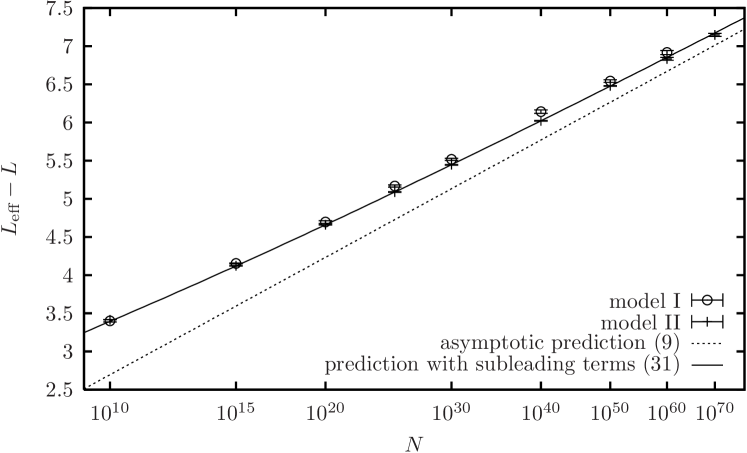
Figure 1: Measured $L_{\text{eff}}$, defined by (30), from which we have subtracted the width $L$ in the cutoff theory, as a function of $N$. The dashed line represents the leading terms $3\log\log N/\gamma_{0}$, see (9). The subleading terms (31) of the plain line have been determined by a fit.

Between times $t$ and $t+1$, $n_{l}(x,t)$ particles out of $n(x,t)$ move to the left and $n_{r}(x,t)$ move to the right. Furthermore, $n_{+}(x,t)$ particles are replaced by their two offsprings at $x$, and $n_{-}(x,t)$ particles disappear. Hence the total variation in the number of particles on site $x$ reads

$$n(x,t+1)-n(x,t)=-n_{l}(x,t)-n_{r}(x,t)-n_{-}(x,t)\\ +n_{+}(x,t)+n_{l}(x+1,t)+n_{r}(x-1,t).$$ (24a)

The numbers describing a timestep at position $$x$$ have a multinomial distribution:

$$P(\{n_{l},n_{r},n_{+},n_{-}\})=\frac{n!}{n_{l}!n_{r}!n_{+}!n_{-}!\Delta n!}p_{l}^{n_{l}}p_{r}^{n_{r}}\\ \lambda^{n_{+}}(\lambda n/N)^{n_{-}}(1\!-\!p_{l}\!-\!p_{r}\!-\!\lambda\!-\!\lambda n/N)^{\Delta n},$$ (24b)

where $\Delta n=n-n_{l}-n_{r}-n_{+}-n_{-}$, and all quantities in the previous equation are understood at site $x$ and time $t$. The mean evolution of $u\equiv n/N$ in one step of time reads

$$\langle u(x,t\!+\!1)|\{u(x,t)\}\rangle\!=\!u(x,t)\!+\!p_{l}[u(x\!+\!1,t)\!-\!u(x,t)]\\ +\!p_{r}[u(x\!-\!1,t)\!-\!u(x,t)]\!+\!\lambda u(x,t)[1\!-\!u(x,t)].$$ (25)

When $N$ is infinitely large, one can replace the $u$’s in (25) by their averages. One obtains then a deterministic front equation in the FKPP class with

$$v(\gamma)=\frac{1}{\gamma}\log\left(1+\lambda+p_{l}(e^{-\gamma}-1)+p_{r}(e^{\gamma}-1)\right),$$ (26)

and $\gamma_{0}$ is defined by $v^{\prime}(\gamma_{0})=0$, see (2).

For the purpose of our numerical study, we set

$$p_{l}=p_{r}=0.1\text{\quad and\quad}\lambda=0.2\,.$$ (27)

From (26), this choice leads to

$$\begin{split}&\gamma_{0}=1.3521\cdots\ ,\ \ v(\gamma_{0})=0.25538\cdots,\\ &v^{\prime\prime}(\gamma_{0})=0.16773\cdots.\end{split}$$ (28)

Predictions for all cumulants of the position of the front are obtained by replacing the values of these parameters in (6).

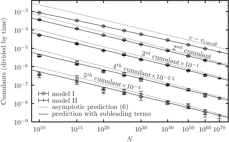
Figure 2: From top to bottom, the correction to the velocity given by the cutoff theory and the cumulants of orders 2 to 5 of the position of the front in the stochastic model. The numerical data are compared to our parameter-free analytical predictions (6), represented by the dashed line. The subleading terms of the plain lines are numerically the same as in figure 1; no further fit has been performed for the present figure.

Technically, in order to be able to go to very large values of $N$, we replace the full stochastic model by its deterministic mean field approximation $u\rightarrow\langle u\rangle$, where $\langle u\rangle$ is given by Eq. (25), in all bins in which the number of particles is larger than $10^{3}$ (that is, in the bulk of the front). Whenever the number of particles is smaller, we use the full stochastic evolution (24). We add an appropriate boundary condition on the interface between the bins described by the deterministic equation and the bins described by the stochastic equation so that the flux of particles is conservedMoro (2004a). This setup will be called “model I”. Eventually, we shall use the mean field approximation everywhere except in the rightmost bin (model II): at each time step, a new bin is filled immediately on the right of the rightmost nonempty site with a number of particles given by a Poisson law of average $\theta=N\langle u(x,t\!+\!1)|\{u(x,t)\}\rangle.$ In the context of a slightly different model in the same universality class Brunet and Derrida (1999), this last approximation was shown numerically to give indistinguishable results from those obtained with the full stochastic version of the model, as far as the front velocity and its diffusion constant were concerned. We shall confirm this observation here.

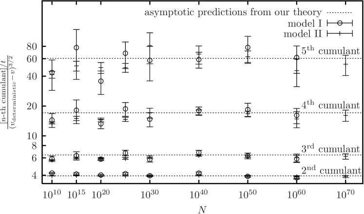
Figure 3: The ratio of cumulants 2 to 5 divided by the correction to the velocity to the power $3/2$. The dashed lines are the analytical prediction assuming only the cutoff theory (5b) for the velocity and the prediction (6) for the cumulants.

We define the position of the front at time $t$ by

$$X_{t}=\sum_{x=0}^{\infty}u(x,t).$$ (29)

We start at time $t=0$ from the initial condition $u(x,0)=1$ for $x\leq 0$ and $u(x,0)=0$ for $x>0$. We evolve it up to time $t=\log^{2}N$ to get rid of subasymptotic effects related to the building of the asymptotic shape of the front, and we measure the mean velocity between times $\log^{2}N$ and $16\times\log^{2}N$. For model I (many stochastic bins), we average the results over $10^{4}$ such realizations. For model II (only one stochastic bin), we generate $10^{5}$ such realizations for $N\leq 10^{50}$ and $10^{4}$ realizations for $N>10^{50}$. In all our simulations, models I and II give numerically indistinguishable results for the values of $N$ where both models were simulated, as can be seen on the figures (results for model I are represented by a circle and for model II by a cross).

First, we check that the effective width of the front is $L_{\text{eff}}$ given by Eq. (9). We extract the latter from the measured mean velocity $v$ using the formula

$$L_{\text{eff}}=\pi\sqrt{\frac{v^{\prime\prime}(\gamma_{0})}{2\big{(}v(\gamma_{0})-v\big{)}}}\ .$$ (30)

We subtract from $L_{\text{eff}}$ the width of the front obtained in the cutoff theory $L=(\log N)/\gamma_{0}$, and compare the numerical result with the analytical formula

$$L_{\text{eff}}-L=\frac{3\log(\log N)}{\gamma_{0}}+c+d\frac{\log(\log N)}{\log N}\ .$$ (31)

The first term in the r.h.s. is suggested by our fourth assumption (see Eq. (9)). We have added two subleading terms which go beyond our theory: a constant term, and a term that vanishes at large $N$. The latter are naturally expected to be the next terms in the asymptotic expansion for large $N$. We include them in this numerical analysis because in the range of $N$ in which we are able to perform our numerical simulations, they may still bring a significant contribution.

We fit (31) to the numerical data obtained in the framework of model II, restricting ourselves to values of $N$ larger than $10^{30}$. In the fit, each data point is weighted by the statistical dispersion of its value in our sample of data. We obtain a determination of the values of the free parameters $c=-4.26\pm 0.01$ and $d=5.12\pm 0.27$, with a good quality of the fit ($\chi^{2}/d.o.f\sim 1.15$). The numerical data together with the theoretical predictions are shown in figure 1. We see a clear convergence of the data to the predicted asymptotics at large $N$ (dotted line in the figure), but subleading corrections that we have accounted for phenomenologically here are sizable over the whole range of $N$.

We now turn to the higher order cumulants. Our numerical data is shown in figure 2 together with the analytical predictions obtained from (6) (dotted lines in the figure). We see that the numerical simulations get very close to the analytical predictions at large $N$. However, like in the case of $L_{\text{eff}}$, higher order corrections are presumably still important for the lowest values of $N$ displayed on the plot.

We try to account for these corrections by replacing the factor $(\log N)/\gamma_{0}=L$ in the denominator of the expression for the cumulants in Eq. (6) by the Ansatz for $L_{\text{eff}}$ given in (31), without retuning the parameters. The results are shown in figure 2 (full lines), and are in excellent agreement with the numerical data over the whole range of $N$. We could also have refitted the parameters $c$ and $d$ for each cumulant separately, as, a priori, they are not predicted by our theory. We observe that this is not required by our data.

This last observation suggests that all the cumulants can be computed, with a good accuracy, with the effective width $L_{\text{eff}}$ as the only parameter. We check this on figure 3, which represents the ratio of the $n$-th cumulant (divided by time) by the correction to the velocity $v_{\text{deterministic}}-v$ to the power $3/2$. If one supposes that the correction to the velocity varies like $1/L_{\text{eff}}^{2}$ and the cumulants like $1/L_{\text{eff}}^{3}$ for some effective width $L_{\text{eff}}$, this width disappears from the ratio plotted and one can compare the numerical results to our analytical prediction with no free parameter or unknown subleading terms. Within statistical error, the data seem to agree for $N$ large enough with our prediction, suggesting that, indeed, all the cumulants can be described with a good accuracy with only the effective width $L_{\text{eff}}$.

Simulations, not shown here, for the model introduced in Brunet and Derrida (1999) support also our predictions (6).

V Conclusion

The main idea that we have put forward in the present work is that all the fluctuations of the front position, and in particular the diffusion constant, are dominated by large but rare fluctuations at the tip of the front.

Under some more precise assumptions (hypotheses of section II) on these fluctuations, we were able to obtain explicit expressions (6) of the cumulants of the position of the front. We checked these predictions in our numerical simulations of section IV. In section III, we gave some arguments in support of the four hypotheses of section II. None of these arguments can be regarded as a mathematical derivation, and we can imagine that some details, such as the precise shape of the distribution of fluctuations (7) or the explicit expression (8), could be slightly modified by a more precise analysis. We believe however, given the good agreement of the predictions (6) with the numerical simulations, that our picture is very close, if not identical, to the actual behavior of the front for large values of $N$.

To conclude, we would like to point out the remarkable similarity between the predictions (6) and the exact results obtained recentlyBrunet and Derrida (2004) in the context of directed polymers. Basically, the results of Brunet and Derrida (2004) are the same, mutatis mutandis as our present results (6), for all the cumulants. The only significant change is that the $3\log\log N$ for the velocity and the $1/\log^{3}N$ dependence for all the cumulants in (6) corresponds, in Brunet and Derrida (2004), to a $\log\log N$ for the velocity and a $1/\log N$ for all the cumulants(Brunet and Derrida, 2004, Eq. (23) with $L=\log N$. The term $L+\log L$ in the velocity corresponds to $v_{\text{cutoff}}$, see Eq. (28)). What is interesting is that our scenario of section II for FKPP fronts applies also for the system studied in Brunet and Derrida (2004): Indeed, the fluctuations of the position are mainly due to the rare big events taking place at the tip of the “front”, (Brunet and Derrida, 2004, last paragraph before conclusion), the position of the rightmost particle is given by (7) (Brunet and Derrida, 2004, Eq. (32) with $\delta=-\log q$ and $X_{t}=\log B_{t}$), the effect of a large fluctuation can be written as (8) with the $L^{3}$ term replaced by $L$ (Brunet and Derrida, 2004, the log of (34) can be written as $X_{t+1}-X_{t}=L+\log L+R(\delta)$), relevant fluctuation (of size $\log L$ instead of $3\log L$) appears every $L$ timesteps (instead of every $L^{3}$ timesteps) and the relaxation time is 1 instead of $L^{2}$. This similarity may add a further piece of evidence for our results.

This work was partially supported by the US Department of Energy.

Appendix A Limit $N\to\infty$

In this appendix, we try to provide an argument for the exponential decay (7) of the distribution for the width of the front. To this aim, we consider a very simple model of reaction-diffusion: particles diffuse on the line and during each time interval $dt$, each particle duplicates with a probability $dt$. The motions of all the particles are uncorrelated.

If one added a saturation rule as described at the beginning of section II, the density of particles (or the number of particles on the right of $x$, depending on the precise saturation rule) would be described by a stochastic FKPP equation. However, the saturation affects only the motion of particles in the bulk of the front, where the density is high. As the fluctuations develop in the low density region, it is reasonable to assume that the distribution of the size of the fluctuations are well described by the model without any saturation.

For this model without saturation, let $P_{t}(x)$ the probability that, at time $t$, no particles are present on the right of $x$ given that, at $t=0$, there is a single particle at the origin: $P_{0}(x)=\theta(x)$. During the first “time step” $dt$, the only particle in the system moves by a quantity $\eta\sqrt{dt}$ where $\eta$ is a Gaussian number of variance $2$, and duplicates with a probability $dt$. If it duplicates, the probability $P_{t+dt}(x)$ is the probability that the offsprings of both particles are on the left of $x$. As the particles have uncorrelated motion, this is the product of the probabilities for each offspring. Finally, one getsMcKean (1975)

$$P_{t+dt}(x)=\left\langle P_{t}(x-\eta\sqrt{dt})(1-dt)+P_{t}^{2}(x-\eta\sqrt{dt})dt\right\rangle,$$

where the average is on $\eta$. After simplification,

$$\partial_{t}P=\partial_{x}^{2}P-P+P^{2}.$$ (32)

One notices that $1-P_{t}(x)$ is solution of the deterministic FKPP equation (1). Therefore, for large $t$ and $x$, Bramson (1983); Brunet and Derrida (1997); van Saarloos (2003)

$$1-P_{t}(x)\sim ze^{-z-\frac{z^{2}}{4t}}\text{\quad for }z=x-2t+\frac{3}{2}\log t.$$

Let $Q_{t}(x)$ be the probability that there are no particles on the right of $x$ when the initial condition is a given density of particles $\rho_{0}(x)$. Using the fact that all the particles are independent, one gets easily

$$Q_{t}(x)=\exp\left[-\int dy\ \rho_{0}(y)\Big{(}1-P_{t}(x-y)\Big{)}\right].$$ (33)

$\rho_{0}(y)$ needs to reproduce the shape of the front seen from the tip. Starting from (5a), we write $\rho(y)=Nh_{\text{cutoff}}(L+y)$ and take the large $N$ limit. One gets $\rho_{0}(y)=-y\exp(-y)$ for $y<0$ and $\rho_{0}(y)=0$ for $y>0$. Evaluating the integral in (33), one gets, for large $t$ and $x-2t\ll\sqrt{t}$,

$$Q_{t}(x)\approx\exp\left[-Ce^{-(x-2t)}\right].$$ (34)

(Notice how the $(3/2)\log t$ factor canceled out). The probability distribution function of the rightmost particle is clearly $\partial_{x}Q_{t}(x)$. We see that in this stochastic model, the front moves at a deterministic velocity equal to $2$ and that the position of the rightmost particle around the position of the front is given by a Gumbel distribution.

The distribution (34) gives our first hypothesis (7) for large fluctuations ($\delta=x-2t\gg 1$). Our attempts to check numerically (34) by simulating fronts with a large but finite number of particles confirmed this exponential decay for large $\delta$, but showed some discrepancy for $\delta<0$, which we do not understand. This, however, does not affect the hypothesis (7).

Appendix B Moving wall

We consider again the reaction-diffusion model introduced in appendix A. As we said, one needs to add a saturation effect to obtain a propagating front equation for the density, but doing so introduces correlations in the motions of the particles that make the model hard to solve. In this appendix, we introduce an approximate way of adding a saturation effect which does not introduce any such correlation.

In a real front, the tip is subject to huge fluctuations happening on short time scales. On the other hand, the bulk of the front moves smoothly and adjusts very slowly to the fluctuations happening at the tip. Therefore, we believe that, for times not too large, it is a reasonable approximation to assume that the bulk of the front moves at a constant velocity.

To implement this idea, our model is the following: a wall starting at the origin is moving to the right at a constant velocity $v$. Particles are present on the right of the wall. The particles are evolving as in appendix A, except that whenever a particle crosses the wall, it is removed.

We first consider a single particle starting at a distance $z$ of the wall. After a time $t$, either all the offsprings of this particle have been caught by the wall, or some have survived. We want to compute the probability $E_{t}(z)$ that all the particles have been caught at time $t$. The original particle, after a time $dt$, is at a distance $z-vdt+\eta\sqrt{dt}$ from the wall, and it might have duplicated with probability $dt$. Using the same method as in appendix A, one gets

$$\partial_{t}E_{t}=\partial_{z}^{2}E_{t}-v\partial_{z}E_{t}-E_{t}+E_{t}^{2}.$$ (35)

with the conditions

$$E_{0}(z)=0\text{ for $z>0$}\quad\text{and}\quad E_{t}(z)=1\text{ for $z<0$}.$$ (36)

In the long time limit, $E_{t}(z)$ converges to the stationary solution $E_{\infty}(z)$, and one recognizes that $h(z)=1-E_{\infty}(-z)$ is the stationary solution of the FKPP equation (1) if $z=x-vt$. In other words, $1-E_{\infty}(-z)$ is the shape of a travelling front. As this shape reaches $0$ for $z=0$, it must be a front with a sine arch and a velocity $v$ smaller than $2$, as in (5). So if $v<2$, the probability $1-E_{\infty}(-z)$ is the shape of the front with a cutoff:

$$1-E(z)\sim Le^{-L}\sin\left(\pi\frac{z}{L}\right)e^{z}\quad\text{where}\quad v=2-\frac{\pi^{2}}{L^{2}}.$$ (37)

(The extra factor $e^{-L}$ comes from the fact that $z=0$ is the tip of the front in (37) while it is the bulk of the front in (5a). If $v>2$, all the particles eventually die and $E_{t}(z)$ converges to $1$.)

If one starts with a density $\rho(z)$ of particles at time $t=0$, the probability $E^{*}_{t}$ that everybody dies is given, similarly to (33), by

$$E^{*}_{t}=\exp\left[-\int_{0}^{+\infty}dz\ \rho(z)\Big{(}1-E_{t}(z)\Big{)}\right].$$ (38)

We consider, as an initial condition, the situation in the real front with $\rho(z)=Nh(z)\sim NL\sin(\pi z/L)\exp(-z)$ for $z<L$ as in (5a). One gets, for long times,

$$E^{*}_{t}\to\exp\left[-{C}NL^{3}e^{-L}\right].$$ (39)

We see that the system survives if

$$NL^{3}e^{-L}\gtrapprox 1\quad\text{or}\quad L\lessapprox\log N+3\log\log N,$$ (40)

which, given $\gamma_{0}=1$, is exactly (9).

References

- Fisher (1937) R. A. Fisher, Annals of Eugenics 7, 355 (1937); A. Kolmogorov, I. Petrovsky, and N. Piscounov, Bull. Univ. État Moscou, A 1, 1 (1937).
- van Saarloos (2003) W. van Saarloos, Phys. Rep. 386, 29 (2003).
- Pechenik and Levine (1999) L. Pechenik and H. Levine, Phys. Rev. E 59, 3893 (1999).
- Doering et al. (2003) C. R. Doering, C. Mueller, and P. Smereka, Physica A 325, 243 (2003).
- Majumdar and Krapivsky (2003) S. N. Majumdar and P. L. Krapivsky, Phys. A 318, 161 (2003).
- Derrida and Spohn (1988) B. Derrida and H. Spohn, J. Stat. Phys. 51, 817 (1988).
- Carpentier and Le Doussal (2000) D. Carpentier and P. Le Doussal, Nucl. Phys. B 588, 531 (2000).
- Munier and Peschanski (2003) S. Munier and R. Peschanski, Phys. Rev. Lett. 91, 232001 (2003).
- Balitsky (1996) I. Balitsky, Nucl. Phys. B 463, 99 (1996); Y. V. Kovchegov, Phys. Rev. D 60, 034008 (1999); Phys. Rev. D 61, 074018 (2000).
- Marquet et al. (2005) C. Marquet, R. Peschanski, and G. Soyez, Nucl. Phys. A 756, 399 (2005).
- Aronson and Weinberger (1975) D. G. Aronson and H. F. Weinberger, Lecture Notes in Mathematics 446, 5 (1975).
- Brunet and Derrida (1997) É. Brunet and B. Derrida, Phys. Rev. E 56, 2597 (1997).
- Enberg et al. (2005) R. Enberg, K. Golec-Biernat, and S. Munier, Phys. Rev. D 72, 074021 (2005).
- Kessler et al. (1998) D. A. Kessler, Z. Ner, and L. M. Sander, Phys. Rev. E 58, 107 (1998).
- Panja (2003) D. Panja, Phys. Rev. E 68, 065202(R) (2003); Phys. Rep. 393, 87 (2004).
- Mueller and Sowers (1995) C. Mueller and R. B. Sowers, J. Funct. Anal. 128, 439 (1995).
- Brunet and Derrida (1999) É. Brunet and B. Derrida, Computer Physics Communications 121–122, 376 (1999); J. Stat. Phys. 103, 269 (2001).
- Mueller and Shoshi (2004) A. H. Mueller and A. I. Shoshi, Nucl. Phys. B 692, 175 (2004).
- Colon and Doering (2005) J. G. Colon and C. R. Doering, J. Stat. Phys. 120, 421 (2005).
- Iancu et al. (2005) E. Iancu, A. H. Mueller, and S. Munier, Phys. Lett. B 606, 342 (2005).
- (21) E. Moro, private discussion.
- Bramson (1983) M. D. Bramson, Mem. Am. Math. Soc. 44 (1983).
- Moro (2004a) E. Moro, Phys. Rev. E 69, 060101(R) (2004a); Phys. Rev. E 70, 045102(R) (2004b).
- Brunet and Derrida (2004) É. Brunet and B. Derrida, Phys. Rev. E 70, 016106 (2004).
- McKean (1975) H. P. McKean, Comm. Pure Appl. Math. 28, 323 (1975).