Transport phenomena in three-dimensional system close to the magnetic quantum critical point: The conserving approximation with the current vertex corrections

Abstract

It is known that various transport coefficients strongly deviate from conventional Fermi-liquid behaviors in many electron systems which are close to antiferromagnetic (AF) quantum critical points (QCP). For example, Hall coefficients and Nernst coefficients in three-dimensional heavy fermion CeCoIn₅ and CeCu_6-xAu_x increase strikingly at low temperatures, whose overall behaviors are similar to those in high-$T_{c}$ cuprates. These temperature dependences are too strong to explain in terms of the relaxation time approximation. To elucidate the origin of these anomalous transport phenomena in three-dimensional systems, we study the current vertex corrections (CVC) based on the fluctuation exchange (FLEX) approximation, and find out decisive role of the CVC. The main finding of the present paper is that the Hall coefficient and the Nernst coefficient strongly increase thanks to the CVC in the vicinity of the AF QCP, irrespective of dimensionality. We also study the relaxation time of quasi-particles, and find that “hot points” and “cold lines” are formed in general three-dimensional systems due to strong AF fluctuations.

I INTRODUCTION

Strongly correlated electron systems close to the quantum critical point (QCP) have stimulated much interest. Especially, heavy fermion compound CeCoIn₅,pet which is a three-dimensional metal close to the antiferromagnetic (AF) QCP, attracts much attention because of the non-Fermi-liquid normal state and the $d$-wave superconductivity ($T_{c}=2.3$K). Moreover, recent experimental efforts have revealed the existence of interesting anomalous transport phenomena characteristic of the AF QCP. In the normal state of CeCoIn₅, for example, it is observed that the resistivitynak $\rho\propto T$, the Hall coefficientnak $R_{H}\propto 1/T$, and the Nernst coefficientbel $\nu\propto 1/T$ below $20$K till $T_{c}=2.3$K. These behaviors are quite different from the normal Fermi-liquid behaviors, $\rho\propto T^{2}$ and $R_{H}\propto T^{0}$.

In Ce115, the maximum values of $R_{H}$ and $\nu$ are quite huge compared to values for high temperatures. The maximum value of $R_{H}$ becomes about $30$ times larger than the values at high temperatures. The value of $\nu$ reaches $-1.0\mu{\rm V/KT}$ at $5$K, whose magnitude is about $1000$ times larger than the values in usual metals. The temperature dependence of $R_{H}$ is similar to the two-dimensional high-$T_{c}$ cuprates above the pseudo-gap temperatures, and that of $\nu$ is similar to electron doped high-$T_{c}$ cuprates, irrespective of signs. Moreover, the magnitude of $R_{H}$ and $\nu$ in CeCoIn₅ is much larger than that in high-$T_{c}$ cuprates. Similar drastic increases of $R_{H}$ are also observed in CeCu_6-xAu_xfuk (a) and YbRh₂Si₂pas , which are three-dimensional heavy fermion compounds close to the AF QCP.

The relaxation time approximation (RTA)sto ; ros has been used frequently in the study of transport phenomena, although its reliability for strongly correlated systems is not assured. According to the spin fluctuation theory, the relaxation time $\tau_{\mbox{\scriptsize\boldmath$k$}}$ becomes strongly anisotropic.hlu ; sto The spots on the Fermi surface where $\tau_{\mbox{\scriptsize\boldmath$k$}}$ takes the maximum (minimum) value is denoted by the cold (hot) spots in literatures. The ratio of the relaxation time at cold spots and hot spots $r=\tau_{\rm cold}/\tau_{\rm hot}$ and the weight of the cold spots play an important role in the transport phenomena. However, in terms of the RTA, an unrealistic huge $r$ (say $r=100$-$1000$) is required to reproduce the experimental enhancement of $R_{H}$ in CeCoIn${}_{5}.$nak If we assume that $R_{H}$ is enhanced by this mechanism, $R_{H}$ should be suppressed quite sensitively by a very small amount of impurity. In addition, when $r\gg 1$, the magnetresistance should be too large to explain the modified Kohler’s rule, $\Delta\rho/\rho\propto R_{H}^{2}/\rho^{2}$, which is observed in high-$T_{c}$ cupratesong (a); and and in CeCoIn₅nak .

These anomalous transport phenomena close to the AF QCP are well reproduced by taking the current vertex corrections (CVC) into account. Actually, the CVC is necessary to satisfy conservation laws. In the Fermi liquid theory, the CVC corresponds to the backflow, which naturally arises from electron-electron correlations. Then, the CVC is indispensable to calculate the transport coefficients in the strongly correlated electron systems, where electron-electron correlations are dominant. For example, the modified Kohler’s rule is explained due to the CVC caused by the AF fluctuations.kon (a) The negative $R_{H}$ in electron doped high-$T_{c}$ cuprates, which cannot be explained by the RTA because the Fermi surface is hole-like everywhere, is explained if we take the CVC. Moreover, it is not easy to explain the enhancement of $\nu$ by the RTA because the Sondheimer cancellationson makes $\nu$ small. The enhancement of $\nu$ in electron-doped (hole-doped) high-$T_{c}$ cuprates are caused by the CVC due to the AF (AF and superconducting) fluctuations.

Until now, various non-Fermi-liquid behaviors of high-$T_{c}$ cuprates have been explained by the spin fluctuation model, such as the self-consistent renormalization (SCR) theorymor (a); ued ; mor (b) and the fluctuation exchange (FLEX) theorybic (a, b); mon . For example, an appropriate behavior of the spin susceptibility and the AF correlation length $\xi$ ($\xi^{2}\propto 1/T$) are obtained. Moreover, spin-fluctuation theoriessto ; mor (b) derive the relation $\rho\propto T^{2}\xi^{2}$, which is consistent with the non-Fermi-liquid behaviors of high-$T_{c}$ cuprates close to the AF QCP. Based on the spin fluctuation theory, Kontani et al.kon (b, a, c, d) have developed a theory of transport phenomena, by focusing on crucial role of the CVC. This framework naturally reproduces the temperature dependence of transport coefficients for high-$T_{c}$ cuprates and other 2D systemskon (e) close to the QCP.

In high-$T_{c}$ cuprateskon (b), the CVC plays an important role on transport phenomena. However, it is highly non-trivial whether the CVC is significant in three-dimensional systems, since the CVC totally vanishes in the dynamical mean field theory (DMFT) where $d=\infty$ limit is taken.kot (a, b) The reason is that the irreducible four-point vertex $\Gamma^{\rm I}$ in the DMFT becomes a local function, which cannot contribute to the CVC. Although it is generally believed that the DMFT works well in various 3D systems with strong correlation,kot (a) the momentum dependences of the self-energy and the vertex corrections are significant near the QCP. However, we must consider the CVC which cannot be taken into account within the DMFT. To elucidate this issue, we study the role of the CVC based on the AF fluctuation theory in three-dimensional systems.

The purpose of this paper is to examine whether non-Fermi-liquid behaviors in 3D systems can be explained by taking account of the CVC in terms of the FLEX approximation. In 3D systems, massive calculation resource and time are needed to perform the calculation. We show that striking increase of $R_{H}$ and $\nu$ can be obtained at low temperatures even in 3D by virtue of the CVC, which is consistent with experiments in CeCoIn₅ and CeCu_6-xAu_x. The present study is the first microscopic calculation for the Hall coefficient and the Nernst coefficient in 3D with the CVC. We also find that in 3D systems, the hot and cold spots form point-like (“hot points”) and line-like shape (“cold lines”), respectively. The CVC on the cold lines plays a major role for increasing $R_{H}$ and $\nu$.

II Formulation

II.1 Model

We first introduce the three-dimensional Hubbard model,

$${\cal H}=-\sum_{i,j}\sum_{\sigma}t_{ij}c_{i\sigma}^{\dagger}c_{j\sigma}+\frac{1}{2}\sum_{i,\sigma}Un_{i\sigma}n_{i-\sigma}$$ (1)

on a stacked square lattice with the Coulomb repulsion $U$ and the intralayer hopping $t_{1}$, $t_{2}$, $t_{3}$ and the interlayer hopping $t_{z}$ depicted in Fig. 1. Hereafter, we take $t_{1}=1$ as a unit of energy.

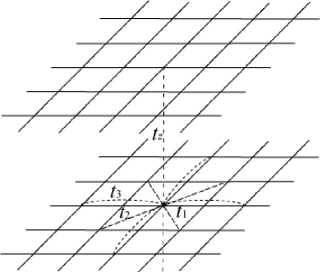
Figure 1: The lattice structure with the nearest intralayer hopping $t_{1}$, the second one $t_{2}$, the third one $t_{3}$ and the interlayer hopping $t_{z}$

Then, the dispersion is derived as,

$$\epsilon^{0}_{\mbox{\scriptsize\boldmath$k$}}=-2t_{1}(\cos(k_{x})+\cos(k_{y}))-4t_{2}\cos(k_{x})\cos(k_{y})$$

$$-2t_{3}(\cos(2k_{x})+\cos(2k_{y}))-2t_{z}\cos(k_{z}).$$ (2)

We apply the FLEX approximationbic (a, b); koi ; kon (f) where the Green’s function, the self-energy and the susceptibility are obtained self-consistently. The FLEX approximation belongs to “conserving approximations” formulated by Baym and Kadanoffbay (a, b). The spin ($\chi^{\rm s}_{\mbox{\scriptsize\boldmath$q$}}$) and charge ($\chi^{\rm c}_{\mbox{\scriptsize\boldmath$q$}}$) susceptibilities are

$$\chi^{\rm s}_{\mbox{\scriptsize\boldmath$q$}}(\omega_{l})=\frac{\chi^{0}_{\mbox{\scriptsize\boldmath$q$}}(\omega_{l})}{1-U\chi^{0}_{\mbox{\scriptsize\boldmath$q$}}(\omega_{l})},$$ (3)

$$\chi^{\rm c}_{\mbox{\scriptsize\boldmath$q$}}(\omega_{l})=\frac{\chi^{0}_{\mbox{\scriptsize\boldmath$q$}}(\omega_{l})}{1+U\chi^{0}_{\mbox{\scriptsize\boldmath$q$}}(\omega_{l})},$$ (4)

and the irreducible susceptibility $\chi^{0}_{\mbox{\scriptsize\boldmath$q$}}$ is

$$\chi^{0}_{\mbox{\scriptsize\boldmath$q$}}(\omega_{l})=-\frac{T}{N}\sum_{{\mbox{\scriptsize\boldmath$k$}},n}G_{\mbox{\scriptsize\boldmath$q$}+\mbox{\scriptsize\boldmath$k$}}(\omega_{l}+\epsilon_{n})G_{\mbox{\scriptsize\boldmath$k$}}(\epsilon_{n}),$$ (5)

where Matsubara frequencies are denoted by $\epsilon_{n}=(2n+1)\pi T$ and $\omega_{l}=2l\pi T$, respectively.

The self-energy is given by

$$\Sigma_{\mbox{\scriptsize\boldmath$k$}}(\epsilon_{n})=\frac{T}{N}\sum_{{\mbox{\scriptsize\boldmath$q$}},l}G_{\mbox{\scriptsize\boldmath$k$}-\mbox{\scriptsize\boldmath$q$}}(\epsilon_{n}-\omega_{l})V_{\mbox{\scriptsize\boldmath$q$}}(\omega_{l}),$$ (6)

where the effective interaction $V_{\mbox{\scriptsize\boldmath$q$}}$ is

$$V_{\mbox{\scriptsize\boldmath$q$}}(\omega_{l})=U^{2}\left(\frac{3}{2}\chi^{\rm s}_{\mbox{\scriptsize\boldmath$q$}}(\omega_{l})+\frac{1}{2}\chi^{\rm c}_{\mbox{\scriptsize\boldmath$q$}}(\omega_{l})-\chi^{0}_{\mbox{\scriptsize\boldmath$q$}}(\omega_{l})\right)+U.$$ (7)

We calculate Green’s function self-consistently with Dyson’s equation,

$$G_{\mbox{\scriptsize\boldmath$k$}}(\epsilon_{n})^{-1}=i\epsilon_{n}+\mu-\epsilon^{0}_{\mbox{\scriptsize\boldmath$k$}}-\Sigma_{\mbox{\scriptsize\boldmath$k$}}(\epsilon_{n}).$$ (8)

The irreducible particle-hole vertex $\Gamma^{\rm I}_{\mbox{\scriptsize\boldmath$kk^{\prime}$}}$ which satisfies $\Gamma^{\rm I}_{\mbox{\scriptsize\boldmath$kk^{\prime}$}}(\epsilon_{n},\epsilon_{n^{\prime}})=\delta\Sigma_{\mbox{\scriptsize\boldmath$k$}}(\epsilon_{n})/\delta G_{\mbox{\scriptsize\boldmath$k^{\prime}$}}(\epsilon_{n^{\prime}})$ is given by

$$\Gamma^{\rm I}_{\mbox{\scriptsize\boldmath$kk^{\prime}$}}(\epsilon_{n},\epsilon_{n^{\prime}})=V_{\mbox{\scriptsize\boldmath$k$}-\mbox{\scriptsize\boldmath$k^{\prime}$}}(\epsilon_{n}-\epsilon_{n^{\prime}})$$ (9)

where the Maki-Thompson term is taken into account and the Aslamazov-Larkin term is omitted because the latter is negligible for the CVC.kon (b)

In this paper we take $N=N_{x}\times N_{y}\times N_{z}=64\times 64\times 32$ $k$-point meshes and the Matsubara frequencies $\epsilon_{n}$ takes the value from $-(2N_{c}-1)\pi T$ to $(2N_{c}-1)\pi T$ with $N_{c}=256$.

II.2 conductivity

In order to derive the transport coefficient, we begin with Kubo formula,

$$\sigma_{\mu\nu}=e^{2}\sum_{{\mbox{\scriptsize\boldmath$kk^{\prime}$}}\sigma\sigma^{\prime}}v^{0}_{{\mbox{\scriptsize\boldmath$k$}}\mu}v^{0}_{{\mbox{\scriptsize\boldmath$k^{\prime}$}}\nu}\left.\frac{{\rm Im}K_{{\mbox{\scriptsize\boldmath$k$}}\sigma,{\mbox{\scriptsize\boldmath$k^{\prime}$}}\sigma^{\prime}}(\omega+i\delta)}{\omega}\right|_{\omega=0},$$ (10)

where $K(\omega+i\delta)$ is analytic continuation of below $K(i\omega)$

$$K_{{\mbox{\scriptsize\boldmath$k$}}\sigma,{\mbox{\scriptsize\boldmath$k^{\prime}$}}\sigma^{\prime}}(i\omega_{n}) = \int^{\beta}_{0}d\tau e^{\omega_{n}\tau}$$ (11)

$$\times\left\langle T_{\tau}\left\{c^{\dagger}_{{\mbox{\scriptsize\boldmath$k$}}\sigma}(\tau)c_{{\mbox{\scriptsize\boldmath$k$}}\sigma}(\tau)c^{\dagger}_{{\mbox{\scriptsize\boldmath$k^{\prime}$}}\sigma^{\prime}}c_{{\mbox{\scriptsize\boldmath$k^{\prime}$}}\sigma^{\prime}}\right\}\right\rangle,$$

and

$$v^{0}_{{\mbox{\scriptsize\boldmath$k$}}\mu}=\frac{\partial\epsilon^{0}_{\mbox{\scriptsize\boldmath$k$}}}{\partial k_{\mu}}.$$ (12)

Eliashbergeli derived the conductivity in this way. By generalizing Eliashberg’s theorykon (e, b) the conductivity is obtained as

$$\sigma_{xx} = e^{2}\sum_{\mbox{\scriptsize\boldmath$k$}}\int\frac{d\epsilon}{\pi}\left(-\frac{\partial f}{\partial\epsilon}\right)\left\{v_{{\mbox{\scriptsize\boldmath$k$}}x}(\epsilon)|G^{\rm R}_{\mbox{\scriptsize\boldmath$k$}}(\epsilon)|^{2}J_{{\mbox{\scriptsize\boldmath$k$}}x}(\epsilon)\right.$$ (13)

$$\left.-{\rm Re}[G^{\rm R}_{\mbox{\scriptsize\boldmath$k$}}(\epsilon)^{2}]\mbox{\boldmath$v$}_{\mbox{\scriptsize\boldmath$k$}x}(\epsilon)^{2}\right\},$$

$$\mbox{\boldmath$v$}_{\mbox{\scriptsize\boldmath$k$}}(\epsilon)=\mbox{\boldmath$\nabla$}[\epsilon^{0}_{\mbox{\scriptsize\boldmath$k$}}+{\rm Re}\Sigma_{\mbox{\scriptsize\boldmath$k$}}(\epsilon)],$$ (14)

where $\mbox{\boldmath$v$}_{\mbox{\scriptsize\boldmath$k$}}$ is the quasi-particle velocity (without $Z$-factor) and the retarded Green’s function $G^{\rm R}_{\mbox{\scriptsize\boldmath$k$}}(\epsilon)$ is derived by the analytic continuation. The total current $\mbox{\boldmath$J$}_{\mbox{\scriptsize\boldmath$k$}}$ is given by the Bethe-Salpeter equation

$$\mbox{\boldmath$J$}_{\mbox{\scriptsize\boldmath$k$}}(\epsilon)=\mbox{\boldmath$v$}_{\mbox{\scriptsize\boldmath$k$}}(\epsilon)+\sum_{\mbox{\scriptsize\boldmath$k^{\prime}$}}\int^{\infty}_{-\infty}\frac{d\epsilon^{\prime}}{4\pi i}{\cal T}_{22}^{\rm I}(\mbox{\boldmath$k$}\epsilon,\mbox{\boldmath$k^{\prime}$}\epsilon^{\prime})|G^{\rm R}_{\mbox{\scriptsize\boldmath$k^{\prime}$}}(\epsilon^{\prime})|^{2}\mbox{\boldmath$J$}_{\mbox{\scriptsize\boldmath$k^{\prime}$}}(\epsilon^{\prime}),$$ (15)

which is based on the Ward identity. The irreducible four-point vertex ${\cal T}^{\rm I}_{lm}(\mbox{\boldmath$k$}\epsilon,\mbox{\boldmath$k$}^{\prime}\epsilon^{\prime})$ is defined in Ref. eli, . According to eq. (9), it is given by

$${\cal T}_{22}^{\rm I}(\mbox{\boldmath$k$}\epsilon,\mbox{\boldmath$k$}^{\prime}\epsilon^{\prime}) = \left({\rm cotanh}\frac{\epsilon^{\prime}-\epsilon}{2T}-{\rm tanh}\frac{\epsilon^{\prime}}{2T}\right)$$ (16)

$$\times 2i{\rm Im}V_{\mbox{\scriptsize\boldmath$k^{\prime}$}-\mbox{\scriptsize\boldmath$k$}}(\epsilon^{\prime}-\epsilon+i\delta).$$

II.3 Hall coefficient

When a weak magnetic field $B$ is induced along $z$ axis, the Hall coefficient $R_{H}$ is given by

$$R_{H}=\frac{\sigma_{xy}/B}{\sigma_{xx}\sigma_{yy}}.$$ (17)

The Hall conductivity $\sigma_{xy}$ is obtained bykoh ; kon (b)

$$\sigma_{xy}/B = -e^{3}\sum_{\mbox{\scriptsize\boldmath$k$}}\int\frac{d\epsilon}{2\pi}\left(-\frac{\partial f}{\partial\epsilon}\right)$$ (18)

$$|{\rm Im}G^{\rm R}_{\mbox{\scriptsize\boldmath$k$}}(\epsilon)||G^{\rm R}_{\mbox{\scriptsize\boldmath$k$}}(\epsilon)|^{2}A_{\mbox{\scriptsize\boldmath$k$}}(\epsilon),$$

$$A_{\mbox{\scriptsize\boldmath$k$}}(\epsilon) = v_{\mbox{\scriptsize\boldmath$k$}x}(\epsilon)\left[J_{\mbox{\scriptsize\boldmath$k$}x}(\epsilon)\frac{\partial J_{\mbox{\scriptsize\boldmath$k$}y}(\epsilon)}{\partial k_{y}}-J_{\mbox{\scriptsize\boldmath$k$}y}(\epsilon)\frac{\partial J_{\mbox{\scriptsize\boldmath$k$}x}(\epsilon)}{\partial k_{y}}\right]$$ (19)

$$+\langle x\leftrightarrow y\rangle,$$

where $f(\epsilon)=1/(\exp(\epsilon/T)+1)$.

II.4 Nernst effect

Nernst coefficient under a weak magnetic field $B$ along $z$ axis and gradient of temperature along $x$ axis is defined as

$$\nu=\frac{-E_{y}}{B\partial_{x}T}.$$ (20)

According to the linear response theorymah , the response function $L^{21}_{\mu\nu}$ is defined as

$$L^{21}_{\mu\nu}(i\omega_{l})=-\frac{T}{\omega_{l}}\int^{\beta}_{0}d\tau e^{i\omega\tau}\langle T_{\tau}j^{Q}_{\mu}(\tau)j_{\nu}(\tau=0)\rangle.$$ (21)

The electron current operator $j$ and the heat current operator $\mbox{\boldmath$j$}^{Q}$ are given by

$$\mbox{\boldmath$j$}=e\sum_{\mbox{\scriptsize\boldmath$k$},\sigma}\mbox{\boldmath$v$}^{0}_{\mbox{\scriptsize\boldmath$k$}}c^{\dagger}_{\mbox{\scriptsize\boldmath$k$},\sigma}c_{\mbox{\scriptsize\boldmath$k$},\sigma},$$ (22)

and

$$\mbox{\boldmath$j$}^{Q}(\omega_{l}) = \lim_{\tau^{\prime}\rightarrow\tau}\sum_{\mbox{\scriptsize\boldmath$k$},\sigma}\int^{\beta}_{0}d\tau e^{i\omega_{l}\tau}$$ (23)

$$\frac{1}{2}\left(\frac{\partial}{\partial\tau}-\frac{\partial}{\partial\tau^{\prime}}\right)c^{\dagger}_{\mbox{\scriptsize\boldmath$k$},\sigma}(\tau)c_{\mbox{\scriptsize\boldmath$k$},\sigma}(\tau^{\prime})$$

$$= \frac{T}{N}\sum_{\mbox{\scriptsize\boldmath$k$},n,\sigma}i(\epsilon_{n}+\omega_{l}/2)\mbox{\boldmath$v$}^{0}_{\mbox{\scriptsize\boldmath$k$}}c^{\dagger}_{\mbox{\scriptsize\boldmath$k$},\sigma}(\epsilon_{n})c_{\mbox{\scriptsize\boldmath$k$},\sigma}(\epsilon_{n}+\omega_{l}),$$ (24)

respectively.

After the analytic continuation for eq. (21), $L^{21}_{xx}$ and $L^{21}_{xy}$ are obtained askon (g)

$$L^{21}_{xx}(+i\delta) = eT\sum_{\mbox{\scriptsize\boldmath$k$}}\int\frac{d\epsilon}{\pi}\left(-\frac{\partial f}{\partial\epsilon}\right)\mbox{\boldmath$q$}_{\mbox{\scriptsize\boldmath$k$}x}(\epsilon)$$ (25)

$$\times\left\{|G^{\rm R}_{\mbox{\scriptsize\boldmath$k$}}(\epsilon)|^{2}J_{\mbox{\scriptsize\boldmath$k$}x}(\epsilon)-{\rm Re}[G^{\rm R}_{\mbox{\scriptsize\boldmath$k$}}(\epsilon)^{2}]\mbox{\boldmath$v$}_{\mbox{\scriptsize\boldmath$k$}x}(\epsilon)\right\},$$

$$L^{21}_{xy}(+i\delta) = BTe^{2}\sum_{\mbox{\scriptsize\boldmath$k$}}\int\frac{d\epsilon}{\pi}\left(-\frac{\partial f}{\partial\epsilon}\right)$$ (26)

$$\times|{\rm Im}G^{\rm R}_{\mbox{\scriptsize\boldmath$k$}}(\epsilon)||G^{\rm R}_{\mbox{\scriptsize\boldmath$k$}}(\epsilon)|^{2}A^{\prime}_{\mbox{\scriptsize\boldmath$k$}}(\epsilon),$$

$$\gamma_{\mbox{\scriptsize\boldmath$k$}}(\epsilon) = -{\rm Im}\Sigma_{\mbox{\scriptsize\boldmath$k$}}(\epsilon),$$ (27)

$$A^{\prime}_{\mbox{\scriptsize\boldmath$k$}}(\epsilon) = \gamma_{\mbox{\scriptsize\boldmath$k$}}(\epsilon)\left\{\mbox{\boldmath$Q$}_{\mbox{\scriptsize\boldmath$k$}}(\epsilon)\times[\mbox{\boldmath$v$}_{\mbox{\scriptsize\boldmath$k$}}(\epsilon)\times\mbox{\boldmath$\nabla$}]_{z}\left[\frac{\mbox{\boldmath$J$}_{\mbox{\scriptsize\boldmath$k$}}(\epsilon)}{\gamma_{\mbox{\scriptsize\boldmath$k$}}(\epsilon)}\right]\right\}_{z},$$ (28)

$$\mbox{\boldmath$Q$}_{\mbox{\scriptsize\boldmath$k$}}(\epsilon) = \mbox{\boldmath$q$}_{\mbox{\scriptsize\boldmath$k$}}(\epsilon)+\sum_{\mbox{\scriptsize\boldmath$k$}^{\prime}}\int\frac{d\epsilon^{\prime}}{4\pi i}$$ (29)

$$\times{\cal T}_{22}^{\rm I}(\mbox{\boldmath$k$}\epsilon,\mbox{\boldmath$k$}^{\prime}\epsilon^{\prime})|G^{\rm R}_{\mbox{\scriptsize\boldmath$k$}^{\prime}}(\epsilon^{\prime})|^{2}\mbox{\boldmath$Q$}_{\mbox{\scriptsize\boldmath$k$}^{\prime}}(\epsilon^{\prime}),$$

where $\mbox{\boldmath$q$}_{\mbox{\scriptsize\boldmath$k$}}$ is the quasi-particle heat velocity $\mbox{\boldmath$q$}_{\mbox{\scriptsize\boldmath$k$}}(\epsilon)=\epsilon\mbox{\boldmath$v$}_{\mbox{\scriptsize\boldmath$k$}}(\epsilon)$.

Using above expressions, $\nu$ can be rewritten as

$$\nu=\frac{L^{21}_{xy}}{BT^{2}\sigma_{xx}}-\frac{S\sigma_{xy}}{B\sigma_{xx}},$$ (30)

where the thermopower $S$ is given by

$$S=\frac{1}{T^{2}}\frac{L^{21}_{xx}}{\sigma_{xx}}.$$ (31)

III Result

Here, we show numerical results obtained by the CVC-FLEX approximation. We use filling $n=0.9$ ($n=1$ corresponds to half filling) and the intralayer hopping parameters $t_{1}=1$, $t_{2}=-1/6$ and $t_{3}=1/5$ which reproduce the Fermi surface of 2D high-$T_{c}$ cuprate YBCO, and introduce the interlayer hopping $t_{z}$ which makes the Fermi surface three-dimensional. The Stoner factor $\alpha_{S}={\rm max}\left\{U\chi_{\mbox{\scriptsize\boldmath$q$}}^{0}(\omega=0)\right\}$ represents the “distance” from the AF order ($\alpha_{S}=1$ corresponds to the boundary of the AF or the spin density wave (SDW) order) since the denominator of the static spin susceptibility is $1-U\chi^{0}$. We calculate for each $t_{z}$ with keeping $\alpha_{S}$, by tuning the value of $U$ as shown by solid line for $\alpha_{S}=0.995$ and dotted line for $\alpha_{S}=0.998$ at $T=0.02$ in Fig. 2. The “distance” from the AF order is considered to be same along these lines. Note that $\alpha_{S}<1$ is always satisfied in 2D ($t_{z}=0$) at finite temperatures reflecting the theory of Mermin-Wagner.mer

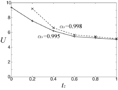
Figure 2: $U$ against $t_{z}$ for $\alpha_{S}=0.995$ (solid line) and $\alpha_{S}=0.998$ (dotted line) at $T=0.02$.

Fig. 3 shows the Fermi surface for $t_{z}=0$ (2D), $t_{z}=0.4$ (quasi-3D; q3D) and $t_{z}=0.8$ (3D). We see that three dimensionality becomes stronger as the value of $t_{z}$ increases. The $k$-dependence of the static spin susceptibility $\chi^{\rm s}_{\mbox{\scriptsize\boldmath$k$}}$ is shown in Fig. 4, where the peak position is commensurate; $(k_{x},k_{y})=(\pi,\pi)$ for $t_{z}=0$ (2D), $(k_{x},k_{y},k_{z})=(\pi,\pi,\pi)$ for $t_{z}=0.4$ (q3D) and incommensurate around $(\pi,\pi,\pi)$ for $t_{z}=0.8$ (3D). From these peak structures, we ensure that the AF fluctuations are dominant in these systems. In this case, the peak values of $\chi^{\rm s}$ increase with $t_{z}$ as seen in Fig. 5. This means that the present system approaches to the AF instability as the dimensionality changes from 2D to 3D.

To understand 3D structure of the relaxation time $\tau$, we show the $k$-dependence of $\gamma_{\mbox{\scriptsize\boldmath$k$}}(=-{\rm Im}\Sigma_{\mbox{\scriptsize\boldmath$k$}}(\epsilon=0))\propto 1/\tau_{\mbox{\scriptsize\boldmath$k$}}$ along the Fermi surface in Figs. 6-8, where hot spots are depicted by circles and cold spots are illustrated by dotted circle. The bottom panels represent the momentum dependence of $\gamma_{\mbox{\scriptsize\boldmath$k$}}$ along the Fermi surface for each $k_{z}$. We see the hot spots exist on the plains of $k_{z}=0$ and $k_{z}=\pi/4$ for $t_{z}=0.4$ and $t_{z}=0.8$, respectively.

The volume fraction of hot spots decreases as $t_{z}$ increases, and for three-dimensional case ($t_{z}=0.8$) hot spots have point-like structure (“hot points”), which is consistent with the experimental result obtained by de Haas-van Alphen measurements on CeIn₃.ebi Generally in 3D systems, nesting exists in only small parts of the Fermi surface, and hot spots form there. In general, the “hot lines”ros where hot spots form line-like structure would not be appropriate in 3D systems.

On the other hand, $\gamma_{k}$ increases more sharply along $k_{\parallel}$ direction than $k_{z}$ direction around minimum point of $\gamma_{k}$ for $t_{z}=0.4$ and $0.8$ as depicted in Fig. 7 and Fig. 8. In this sense, cold spots stretch strikingly along $k_{z}$ direction. Then, cold spots form line-like structure (“cold lines”). They are aligned perpendicular to the plain with hot spots. The formation of hot points and cold lines would be generally expected in three-dimensional systems. To confirm the generality, we must study much more systems with various types of 3D Fermi surfaces.

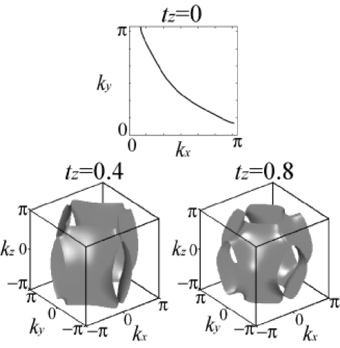
Figure 3: Fermi surface for 2D with $t_{z}=0$ (upper panel), q3D with $t_{z}=0.4$ (lower left panel) and 3D with $t_{z}=0.8$ (lower right panel) for $T=0.02$, $\alpha_{S}=0.995$.

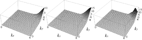
Figure 4: The spin susceptibility for $t_{z}=0$ (left panel), $0.4$ (middle panel) with $k_{z}=\pi$, $0.8$ (right panel) with $k_{z}=\pi$ , for $\alpha_{S}=0.995$, $T=0.02$.

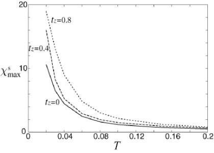
Figure 5: The temperature dependence of the peak value of spin susceptibility for $t_{z}=0$, $0.4$, $0.8$, in the condition of $\alpha_{S}=0.995$ at $T=0.02$.

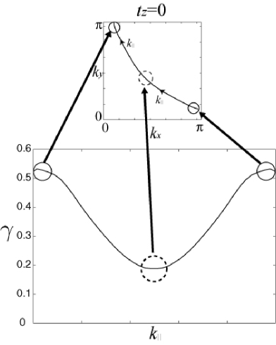
Figure 6: $\gamma$ along the Fermi surface for $t_{z}=0$, $\alpha_{S}=0.995$ at $T=0.02$, where the hot spots and cold spots are depicted by solid circles and dotted circle, respectively.

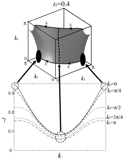
Figure 7: $\gamma$ along the Fermi surface for $t_{z}=0.4$, $\alpha_{S}=0.995$ at $T=0.02$, where the hot spots and the “cold lines” are depicted by circles and dotted thick line, respectively. The trajectories of $k_{\parallel}$ are depicted on the Fermi surface in $k_{z}=0,\pi$ as examples.

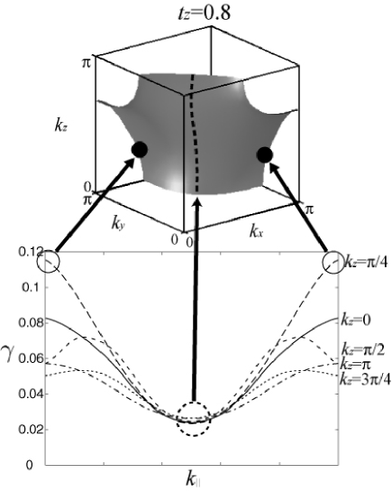
Figure 8: $\gamma$ along the Fermi surface for $t_{z}=0.8$, $\alpha_{S}=0.995$, at $T=0.02$ where the hot spots and the “cold lines” are depicted by circles and dotted thick line, respectively.

The calculated temperature dependence of the resistivity $\rho=1/\sigma_{xx}$ for $t_{z}=0$ (2D), $t_{z}=0.4$ (q3D) and $t_{z}=0.8$ (3D) with $U=9.4$, $U=6.2$ and $U=5.2$, respectively (see Fig. 2), are shown in Fig. 9, where the unit of $\rho$ is $\frac{\hbar a_{c}}{e^{2}}\sim 2.4\times 10^{-6}\Omega\rm{m}$ for a bilayer YBCO (lattice constant along $c$ axis : $a_{c}=5.8\times 10^{-10}$m) and $3.1\times 10^{-6}\Omega\rm{m}$ for CeCoIn₅ ($a_{c}=7.6\times 10^{-10}$m), respectively. The value of $U$ is chosen to satisfy $\alpha_{S}=0.995$ at $T=0.02$ for each case. In this case, the “distance” from the AF QCP is the same among three $t_{z}$ parameters. We see that, independently of the dimensionality, the resistivities with and without the CVC are proportional to the temperature. Then, the value of $\rho$ is slightly enhanced by the CVC. It decreases as $t_{z}$ increases since the corresponding value of $U$ is reduced. This $T$-liner behavior of the resistivity is consistent with experiments for the systems close to the AF QCP, such as two-dimensional high-$T_{c}$ cuprate and three-dimensional CeCoIn₅nak . In detail, the resistivities with the CVC show sub-liner temperature dependence in low temperatures, which are also observed in the experimental results for heavy fermion CeRhIn₅ (private discussion). According to the SCR theory,mor (b, c) the resistivity behaves as $\rho\propto T$ in 2D, and $\rho\propto T^{3/2}$ in 3D. However, the SCR theory also predicts that $\rho\propto T$ for a wide range of temperatures even in 3D systems when the system is close to the AF QCP, which is consistent with the present numerical calculation.

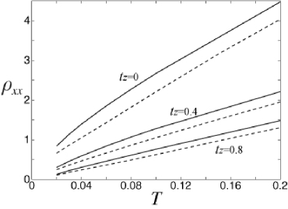
Figure 9: The resistivity $\rho$ with the CVC (solid line) and without the CVC (dotted line) for $t_{z}=0$, $0.4$, $0.8$ as a function of $T$ with $\alpha_{S}=0.995$ at $T=0.02$.

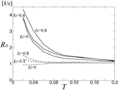
Figure 10: The Hall coefficient $R_{H}$ with the CVC (solid line) and without the CVC (dotted line) for $t_{z}=0$, $0.4$, $0.8$ as a function of $T$, with $\alpha_{S}=0.995$ at $T=0.02$.

Next, we show the temperature dependence of the Hall coefficient $R_{H}$ in Fig. 10, where the unit of $R_{H}$ is $\frac{a_{a}a_{b}a_{c}}{e}\sim 5.2\times 10^{-10}\rm{m}^{3}/\rm{C}$ for a bilayer YBCO (lattice constant along $a$ and $b$ axis : $a_{a}=a_{b}=3.8\times 10^{-10}$m and that along $c$ axis : $a_{c}=5.8\times 10^{-10}$m) and $1.0\times 10^{-9}\rm{m}^{3}/\rm{C}$ for CeCoIn₅ ($a_{a}=a_{b}=4.6\times 10^{-10}$m and $a_{c}=7.6\times 10^{-10}$m), respectively. In regard to the horizontal axis, unit of the temperature $t_{1}$ is $4000$K for YBCO. On the other hand, we estimate the nearest neighbor hopping $t_{1}=400$K for CeCoIn₅, because the experimetal datanak shows that magnitude of $R_{H}$ begins to increase below $40$K, which corresponds to $0.1t_{1}$ in Fig. 10. The $R_{H}$ without the CVC, which corresponds to the RTA, is almost constant. However, independently of the dimensionality, $R_{H}$ with the CVC increases as temperature decreases, which is consistent with experimental results for high-$T_{c}$ cupratetak and heavy fermion compounds (CeCoIn₅nak , CeCu_6-xAu_xfuk (a) and YbRh₂Si₂pas ). Namely, the RTA cannot explain the strong temperature dependence of the Hall coefficient close to the AF QCP. Moreover, in 3D case hot spots take point-like shape, which means that the effective electron density for transport phenomena ($n_{\rm eff}$) is large compared with two-dimensional case. Since $R_{H}^{\rm RTA}\approx\frac{1}{en_{\rm eff}}$ is satisfied in the RTA, $R_{H}^{\rm eff}$ cannot become large in 3D systems.

As a result, the CVC is indispensable to explain the behavior of $R_{H}$ in 3D close to the AF QCP. In the present results, the maximum enhancement of $R_{H}$ is given by $R_{H}(T=0.02)/R_{H}(t=0.2)\sim 5$ for $t_{z}=0.8$ and $\alpha_{S}=0.998$. $R_{H}$ should increase further if we calculate at lower temperatures. The shape of the Fermi surface in CeCoIn₅ resembles to that of our model for $t_{z}=0.8$. However, to reproduce the experimental results in CeCoIn₅ quantitatively, we have to study it based on the realistic band structures of CeCoIn₅.mae ; har Our calculation shows that $R_{H}$ is strongly enhanced by the CVC even in 3D systems, and its maximum value becomes as large as that in 2D.

Here, we discuss the reason why $R_{H}$ is strongly enhanced by the CVC in 3D systems based on the numerical study. The general expression for $\sigma_{xy}$ is given bykoh ; fuk (b)

$$\sigma_{xy}/B=-\frac{e^{3}}{8\pi}\int dk_{z}\oint_{\rm FS}dk_{\parallel}|\mbox{\boldmath$J$}_{\mbox{\scriptsize\boldmath$k$}}|_{\perp}^{2}\left(\frac{\partial\theta_{\mbox{\scriptsize\boldmath$J$}}(\mbox{\boldmath$k$})}{\partial k_{\parallel}}\right)\frac{1}{(\gamma_{\mbox{\scriptsize\boldmath$k$}})^{2}},$$ (32)

where $k_{\parallel}$ is the component of $k$ along the unit vector $\mbox{\boldmath$e$}_{\parallel}(\mbox{\boldmath$k$})=(\mbox{\boldmath$e$}_{z}\times\mbox{\boldmath$v$}_{\mbox{\scriptsize\boldmath$k$}})/|\mbox{\boldmath$v$}_{\mbox{\scriptsize\boldmath$k$}}|$ which is in the $k_{x}k_{y}$-plane and parallel to the Fermi surface. $|\mbox{\boldmath$J$}_{\mbox{\scriptsize\boldmath$k$}}|_{\perp}=\sqrt{J_{\mbox{\scriptsize\boldmath$k$}x}^{2}+J_{\mbox{\scriptsize\boldmath$k$}y}^{2}}$, and $\theta_{\mbox{\scriptsize\boldmath$J$}}$ is the angle between the total current $J$ and the $x$ axis. In this line integration $k$-point moves anticlockwise along the Fermi surface around the $k_{z}$ axis.

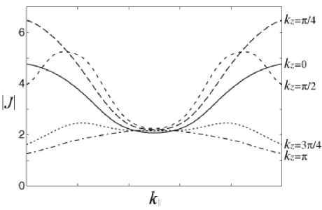
Figure 11: Absolute value of the total current $J$ with the CVC along the Fermi surface for $t_{z}=0.8$ and $t_{z}=0$ (thin line) with $\alpha_{S}=0.995$ at $T=0.02$.

We see that for $t_{z}=0.8$, cold spots (where $\gamma_{\mbox{\scriptsize\boldmath$k$}}$ is small) form lines (cold lines) at the center of the Fermi surface along the $z$ axis in Fig. 8. As shown in the last term of eq. (32), main contribution for $\sigma_{xy}$ is expected to come from the cold lines. We see that in Fig. 11 the momentum dependence of the absolute value of the total current $|\mbox{\boldmath$J$}_{\mbox{\scriptsize\boldmath$k$}}|$ is quite similar to that of $\gamma_{\mbox{\scriptsize\boldmath$k$}}$.

In Fig. 12, we plot $\theta_{J}$ along the trajectories of $k_{\parallel}$. As references, we also plot the corresponding quantity without the CVC, $\theta_{\mbox{\scriptsize\boldmath$v$}}$ for $k_{z}=0$-$\pi/2$ and $k_{z}=3\pi/4$-$\pi$ as a thin line and a dotted thin line, respectively. As show in Fig. 12, $\theta_{\mbox{\scriptsize\boldmath$v$}}$ for $k_{z}=0$-$\pi/2$ and $k_{z}=3\pi/4$-$\pi$ decrease and increase, respectively, along the trajectories of $k_{\parallel}$. On the other hand, $\theta_{\mbox{\scriptsize\boldmath$J$}}$ has a non-monotonic change along these trajectories. Especially, for $k_{z}=3\pi/4$-$\pi$ $\theta_{\mbox{\scriptsize\boldmath$J$}}$ decreases contrary to the case of $\theta_{v}$. We stress that the magnitude of $\partial\theta_{\mbox{\boldmath$J$}}/\partial k_{\parallel}$ becomes larger than that without the CVC ($\partial\theta_{\mbox{\boldmath$v$}}/\partial k_{\parallel}$)around the cold lines.

In Fig. 13, we plot the momentum resolved Hall conductivity $\sigma_{xy}(\mbox{\boldmath$k$})$ defined by $\sigma_{xy}=\sum_{\mbox{\scriptsize\boldmath$k$}}\sigma_{xy}(\mbox{\boldmath$k$})$, where $\sigma_{xy}(\mbox{\boldmath$k$})$ is given by $\sigma_{xy}(\mbox{\boldmath$k$})=-\int\frac{d\epsilon}{2\pi N}\left(-\frac{\partial f}{\partial\epsilon}\right)|{\rm Im}G^{\rm R}_{\mbox{\scriptsize\boldmath$k$}}(\epsilon)||G^{\rm R}_{\mbox{\scriptsize\boldmath$k$}}(\epsilon)|^{2}A_{\mbox{\scriptsize\boldmath$k$}}(\epsilon)$. The magnitude of $\sigma_{xy}(\mbox{\boldmath$k$})$ takes large values around the cold lines , especially for $k_{z}=-\pi/2$-$\pi/2$. We should comment that for $k_{z}=3\pi/4,\pi$ the difference of the value of $\theta_{\mbox{\scriptsize\boldmath$v$}}$ and $\theta_{\mbox{\scriptsize\boldmath$J$}}$ becomes $\pi$ at the edge of the trajectory as shown in Fig. 12 due to the CVC. At that time, the direction of $\mbox{\boldmath$J$}_{\mbox{\scriptsize\boldmath$k$}}$ is opposite to that of $\mbox{\boldmath$v$}_{\mbox{\scriptsize\boldmath$k$}}$. In this case, strong AF spin fluctuation enhances the magnitude of ${\cal T}^{\rm I}_{22}(\mbox{\boldmath$k$}\epsilon,\mbox{\boldmath$k^{\prime}$}\epsilon^{\prime})$ in the eq. (15) for $\mbox{\boldmath$k$}-\mbox{\boldmath$k$}^{\prime}=\pm(\pi,\pi,\pi)$, $\pm(-\pi,\pi,\pi)$, $\pm(\pi,-\pi,\pi)$ and $\pm(\pi,\pi,-\pi)$. In this case, from eq. (15), we can obtain $\mbox{\boldmath$J$}_{\mbox{\scriptsize\boldmath$k$}}\approx\mbox{\boldmath$v$}_{\mbox{\scriptsize\boldmath$k$}}+\alpha_{\mbox{\scriptsize\boldmath$k$}}\mbox{\boldmath$J$}_{\mbox{\scriptsize\boldmath$k^{\prime}$}}$ ($0<\alpha\leq 1$) kon (b). This equation is easily solved as

$$\mbox{\boldmath$J$}_{\mbox{\scriptsize\boldmath$k$}}=\frac{\mbox{\boldmath$v$}_{\mbox{\scriptsize\boldmath$k$}}+\alpha_{\mbox{\scriptsize\boldmath$k$}}\mbox{\boldmath$v$}_{\mbox{\scriptsize\boldmath$k^{\prime}$}}}{1-\alpha_{\mbox{\scriptsize\boldmath$k$}}\alpha_{\mbox{\scriptsize\boldmath$k^{\prime}$}}}.$$ (33)

In Fig. 14, we illustrate schematic behaviors of the quasi-particle velocity $\mbox{\boldmath$v$}_{\mbox{\scriptsize\boldmath$k$}}$ and the total current $\mbox{\boldmath$J$}_{\mbox{\scriptsize\boldmath$k$}}$ on the Fermi surfaces sliced at $k_{z}=\pi$ (solid circle) and at $k_{z}=0$ (dotted circle). We focus on the position of points A and B, which are connected by the nesting vector $\mbox{\boldmath$k$}-\mbox{\boldmath$k$}^{\prime}=(-\pi,-\pi,\pi)$. Here, we write the quasi-particle velocities at A and B as $\mbox{\boldmath$v$}_{\mbox{\scriptsize\boldmath$k$}}$ and $\mbox{\boldmath$v$}_{\mbox{\scriptsize\boldmath$k^{\prime}$}}$, respectively. We see that $\mbox{\boldmath$v$}_{\mbox{\scriptsize\boldmath$k$}}$ and $\mbox{\boldmath$v$}_{\mbox{\scriptsize\boldmath$k^{\prime}$}}$ are antiparallel and $|\mbox{\boldmath$v$}_{\mbox{\scriptsize\boldmath$k$}}|<|\mbox{\boldmath$v$}_{\mbox{\scriptsize\boldmath$k^{\prime}$}}|$. Considering that $\alpha\lesssim 1$, $\mbox{\boldmath$J$}_{\mbox{\scriptsize\boldmath$k$}}$ given in eq. (33) takes an opposite direction of $\mbox{\boldmath$v$}_{\mbox{\scriptsize\boldmath$k$}}$. In the same way, the total current and the quasi-particle velocity at C are also antiparallel. This nontrivial behavior of $\mbox{\boldmath$J$}_{\mbox{\scriptsize\boldmath$k$}}$ has not been pointed out in previous studies for two-dimensional systems. This feature might induce an anomalous transport phenomenon.

In Fig. 15, we show the temperature dependence of $R_{H}$ for $\alpha_{S}=0.998$ (solid line) and $\alpha_{S}=0.995$ (dotted line) for $t_{z}=0.4$ and $0.8$. We see that $R_{H}$ with the CVC increases as $\alpha_{S}$ approaches unity. It seems that $R_{H}$ tends to diverge as the system approaches the AF QCP. The reason can be understood by seeing Fig. 16, where $\partial\theta_{\mbox{\scriptsize\boldmath$J$}}/\partial k_{\parallel}$ takes a large value at the cold spot which corresponds to the center of the $k_{\parallel}$ axis. According to eq. (32), this fact leads to the strong enhancement of $\sigma_{xy}$.

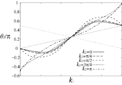
Figure 12: the angle $\theta_{\mbox{\scriptsize\boldmath$J$}}$ of the total current $J$ with the CVC along the Fermi surface for $t_{z}=0.8$, $\alpha_{S}=0.995$ at $T=0.02$. Thin line and dotted thin line approximately correspond to the angle $\theta_{\mbox{\scriptsize\boldmath$v$}}$ of the current without the CVC for $k_{z}=0$-$\pi/2$ and $k_{z}=3\pi/4$-$\pi$, respectively

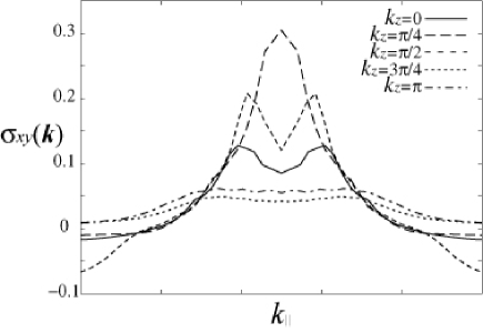
Figure 13: $\sigma_{xy}(\mbox{\boldmath$k$})$ along the Fermi surface for $t_{z}=0.8$, $\alpha_{S}=0.995$ at $T=0.02$.

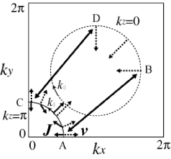
Figure 14: Schematic illustration to show that at A and B $\mbox{\boldmath$J$}_{\mbox{\scriptsize\boldmath$k$}}$ can direct opposite to $\mbox{\boldmath$v$}_{\mbox{\scriptsize\boldmath$k$}}$, where the Fermi surface for $k_{z}=0,\pi$ are depicted by dotted and solid circle, respectively, and $\mbox{\boldmath$J$}_{\mbox{\scriptsize\boldmath$k$}}$ and $\mbox{\boldmath$v$}_{\mbox{\scriptsize\boldmath$k$}}$ are by solid and dotted arrows, and the thick left-right arrows represent the coupling points.

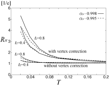
Figure 15: The Hall coefficient $R_{H}$ with the CVC (upside) and without the CVC (downside) for $t_{z}=0.4$, $0.8$ as a function of $T$ with $\alpha_{S}=0.995$ (solid line), $0.998$ (dotted line) at $T=0.02$.

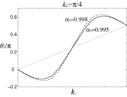
Figure 16: the angle $\theta_{\mbox{\scriptsize\boldmath$J$}}$ of the total current $J$ with the CVC along the Fermi surface for $t_{z}=0.8$, $k_{z}=\pi/4$, $\alpha_{S}=0.995$ (solid line) and $\alpha_{S}=0.998$ (dotted line) at $T=0.02$. Thin line approximately corresponds to one without the CVC.

Finally, we discuss the Nernst coefficient $\nu$. It is known that $\nu$ vanishes in a complete spherical system, which is called Sondheimer cancellation.son ; ong (b) Although this cancellation is not perfect in real anisotropic systems, the magnitude of $\nu$ becomes small ($\sim 1{\rm nV/KT}$) in conventional metals.

However, $\nu$ is enhanced below $T^{*}$ (in the pseudo-gap region) for high-$T_{c}$ cuprates. The authors of Refs. ong, c, b suggest a possibility that the vortex-like excitation emerges in under-doped high-$T_{c}$ cuprates to explain the enhancement of $\nu$ in the pseudo-gap region.

On the other hand, one of the present authorkon (d, h) has shown that strong enhancement of $\nu$ for high-$T_{c}$ cuprates is naturally derived based on the FLEX+T-matrix approximation with the CVC. Furthermore, CeCoIn₅ also shows huge negative $\nu$ below $20$K,bel which cannot be ascribed to the vortex mechanism. Here, we aim to reveal the mechanism of the unconventional enhancement for $\nu$ close to the QCP irrespective of the dimensionality.

We estimate the renormalization factor ($z$) dependence of the transport coefficients, before showing the result of $\nu$. In the following, we will show that $\rho$ and $R_{H}$ are independent of $z$, and $\nu\propto z^{-1}$ in Hubbard model. Using the relationkon (g)

$$\sum_{\mbox{\scriptsize\boldmath$k$}}=\frac{1}{(2\pi)^{3}}\int dS_{\mbox{\scriptsize\boldmath$k$}}dk_{\perp}=\frac{1}{(2\pi)^{3}}\int\frac{dS_{\mbox{\scriptsize\boldmath$k$}}d\epsilon^{0}_{\mbox{\scriptsize\boldmath$k$}}}{|\mbox{\boldmath$v$}^{0}_{\mbox{\scriptsize\boldmath$k$}}|}=\frac{1}{(2\pi)^{3}}\int\frac{dS_{\mbox{\scriptsize\boldmath$k$}}d\epsilon^{*}_{\mbox{\scriptsize\boldmath$k$}}}{z|\mbox{\boldmath$v$}_{\mbox{\scriptsize\boldmath$k$}}|},$$ (34)

where $S_{\mbox{\scriptsize\boldmath$k$}}$ is the Fermi surface and $k_{\perp}$ represents the momentum perpendicular to the Fermi surface and also using the relation $|G^{\rm R}_{\mbox{\scriptsize\boldmath$k$}}(\epsilon)|^{2}\sim\pi z\delta(\epsilon-\epsilon^{*}_{\mbox{\scriptsize\boldmath$k$}})/\gamma_{\mbox{\scriptsize\boldmath$k$}}$ ($\epsilon^{*}_{\mbox{\scriptsize\boldmath$k$}}=z(\epsilon^{0}_{\mbox{\scriptsize\boldmath$k$}}+\rm{Re}\Sigma_{\mbox{\scriptsize\boldmath$k$}}(0)-\mu)$) for $\gamma\ll T$, we obtain

$$\sigma_{xx} \sim \frac{e^{2}}{(2\pi)^{3}}\int\frac{dS_{\mbox{\scriptsize\boldmath$k$}}d\epsilon^{*}_{\mbox{\scriptsize\boldmath$k$}}}{z|\mbox{\boldmath$v$}_{\mbox{\scriptsize\boldmath$k$}}|}\left(-\frac{\partial f}{\partial\epsilon}\right)_{\epsilon=\epsilon^{*}_{\mbox{\scriptsize\boldmath$k$}}}\mbox{\boldmath$v$}_{\mbox{\scriptsize\boldmath$k$}x}\mbox{\boldmath$J$}_{\mbox{\scriptsize\boldmath$k$}x}\frac{z}{\gamma_{\mbox{\scriptsize\boldmath$k$}}}$$ (35)

$$\propto (z)^{0}.$$ (36)

In the same way, $\sigma_{xy}$ is given by,

$$\sigma_{xy} \sim \frac{e^{3}B}{4(2\pi)^{3}}\int\frac{dS_{\mbox{\scriptsize\boldmath$k$}}d\epsilon^{*}_{\mbox{\scriptsize\boldmath$k$}}}{z|\mbox{\boldmath$v$}_{\mbox{\scriptsize\boldmath$k$}}|}\left(-\frac{\partial f}{\partial\epsilon}\right)_{\epsilon=\epsilon^{*}_{\mbox{\scriptsize\boldmath$k$}}}A_{\mbox{\scriptsize\boldmath$k$}}\frac{z}{\gamma_{\mbox{\scriptsize\boldmath$k$}}^{2}}$$ (37)

$$\propto (z)^{0}.$$ (38)

We see that $\sigma_{xx}$ and $\sigma_{xy}$ are independent of $z$. Thus, we confirm that $\rho=1/\sigma_{xx}\propto(z)^{0}$ and $R_{H}=\frac{\sigma_{xy}}{B\sigma_{xx}^{2}}\propto(z)^{0}$ are independent of $z$. On the other hand, thermopower $S$ is given by

$$S \sim \frac{e}{(2\pi)^{3}T\sigma_{xx}}\int\frac{dS_{\mbox{\scriptsize\boldmath$k$}}d\epsilon^{*}_{\mbox{\scriptsize\boldmath$k$}}}{z|\mbox{\boldmath$v$}_{\mbox{\scriptsize\boldmath$k$}}|}\left(-\frac{\partial f}{\partial\epsilon}\right)_{\epsilon=\epsilon^{*}_{\mbox{\scriptsize\boldmath$k$}}}\epsilon^{*}_{\mbox{\scriptsize\boldmath$k$}}\mbox{\boldmath$v$}_{\mbox{\scriptsize\boldmath$k$}x}\mbox{\boldmath$J$}_{\mbox{\scriptsize\boldmath$k$}x}\frac{z}{\gamma_{\mbox{\scriptsize\boldmath$k$}}}$$ (39)

$$= \frac{e}{(2\pi)^{3}T\sigma_{xx}}\int\frac{dS_{\mbox{\scriptsize\boldmath$k$}}d\epsilon^{*}_{\mbox{\scriptsize\boldmath$k$}}}{z|\mbox{\boldmath$v$}_{\mbox{\scriptsize\boldmath$k$}}|}\left(-\frac{\partial f}{\partial\epsilon}\right)_{\epsilon=\epsilon^{*}_{\mbox{\scriptsize\boldmath$k$}}}\!\!\!\!\!\!\!\!\!\!(\epsilon^{*}_{\mbox{\scriptsize\boldmath$k$}})^{2}\frac{\partial}{\partial k_{\perp}}\left(\frac{\mbox{\boldmath$v$}_{\mbox{\scriptsize\boldmath$k$}x}\mbox{\boldmath$J$}_{\mbox{\scriptsize\boldmath$k$}x}}{|\mbox{\boldmath$v$}_{\mbox{\scriptsize\boldmath$k$}}|\gamma_{\mbox{\scriptsize\boldmath$k$}}}\right)_{\epsilon=0}$$ (40)

$$= \frac{e\pi^{2}k_{B}^{2}T}{3(2\pi)^{3}\sigma_{xx}}\int\frac{dS_{\mbox{\scriptsize\boldmath$k$}}}{z|\mbox{\boldmath$v$}_{\mbox{\scriptsize\boldmath$k$}}|}\frac{\partial}{\partial k_{\perp}}\left(\frac{\mbox{\boldmath$v$}_{\mbox{\scriptsize\boldmath$k$}x}\mbox{\boldmath$J$}_{\mbox{\scriptsize\boldmath$k$}x}}{|\mbox{\boldmath$v$}_{\mbox{\scriptsize\boldmath$k$}}|\gamma_{\mbox{\scriptsize\boldmath$k$}}}\right)_{\epsilon=0}$$ (41)

$$\propto z^{-1},$$ (42)

and using $Q_{\mbox{\scriptsize\boldmath$k$}}\sim\mbox{\boldmath$q$}_{\mbox{\scriptsize\boldmath$k$}}=\epsilon\mbox{\boldmath$v$}_{\mbox{\scriptsize\boldmath$k$}}$ for $T\rightarrow 0$, $\alpha_{xy}=L^{21}_{xy}(+i\delta)/T^{2}$ is given by

$$\alpha_{xy} \sim \frac{Be^{2}}{2(2\pi)^{3}T}\int\frac{dS_{\mbox{\scriptsize\boldmath$k$}}d\epsilon^{*}_{\mbox{\scriptsize\boldmath$k$}}}{z|\mbox{\boldmath$v$}_{\mbox{\scriptsize\boldmath$k$}}|}\left(-\frac{\partial f}{\partial\epsilon}\right)_{\epsilon=\epsilon^{*}_{\mbox{\scriptsize\boldmath$k$}}}\epsilon^{*}_{\mbox{\scriptsize\boldmath$k$}}A^{\prime\prime}_{\mbox{\scriptsize\boldmath$k$}}(\epsilon^{*}_{\mbox{\scriptsize\boldmath$k$}})\frac{z}{\gamma^{2}_{\mbox{\scriptsize\boldmath$k$}}}$$ (43)

$$= \frac{Be^{2}}{2(2\pi)^{3}T}\int\frac{dS_{\mbox{\scriptsize\boldmath$k$}}d\epsilon^{*}_{\mbox{\scriptsize\boldmath$k$}}}{z|\mbox{\boldmath$v$}_{\mbox{\scriptsize\boldmath$k$}}|}\left(-\frac{\partial f}{\partial\epsilon}\right)_{\epsilon=\epsilon^{*}_{\mbox{\scriptsize\boldmath$k$}}}\!\!\!\!\!\!\!\!\!\!(\epsilon^{*}_{\mbox{\scriptsize\boldmath$k$}})^{2}\frac{\partial}{\partial k_{\perp}}\left(\frac{A^{\prime\prime}_{\mbox{\scriptsize\boldmath$k$}}}{|\mbox{\boldmath$v$}_{\mbox{\scriptsize\boldmath$k$}}|\gamma^{2}_{\mbox{\scriptsize\boldmath$k$}}}\right)_{\epsilon=0}$$ (44)

$$= \frac{Be^{2}\pi^{2}k_{B}^{2}T}{6(2\pi)^{3}}\int\frac{dS_{\mbox{\scriptsize\boldmath$k$}}}{z|\mbox{\boldmath$v$}_{\mbox{\scriptsize\boldmath$k$}}|}\frac{\partial}{\partial k_{\perp}}\left(\frac{A^{\prime\prime}_{\mbox{\scriptsize\boldmath$k$}}}{|\mbox{\boldmath$v$}_{\mbox{\scriptsize\boldmath$k$}}|\gamma^{2}_{\mbox{\scriptsize\boldmath$k$}}}\right)_{\epsilon=0}$$ (45)

$$\propto z^{-1},$$ (46)

where $A^{\prime\prime}_{\mbox{\scriptsize\boldmath$k$}}(\epsilon)$ is defined by

$$A^{\prime\prime}_{\mbox{\scriptsize\boldmath$k$}}(\epsilon)=\gamma_{\mbox{\scriptsize\boldmath$k$}}(\epsilon)\left\{\mbox{\boldmath$v$}_{\mbox{\scriptsize\boldmath$k$}}(\epsilon)\times[\mbox{\boldmath$v$}_{\mbox{\scriptsize\boldmath$k$}}(\epsilon)\times\mbox{\boldmath$\nabla$}]_{z}\left[\frac{\mbox{\boldmath$J$}_{\mbox{\scriptsize\boldmath$k$}}(\epsilon)}{\gamma_{\mbox{\scriptsize\boldmath$k$}}(\epsilon)}\right]\right\}_{z}$$ (47)

Thus, we obtain $\nu=\frac{\alpha_{xy}}{B\sigma{xx}}-\frac{S\sigma_{xy}}{B\sigma_{xx}}\propto z^{-1}$. We must consider $z$ in detail to calculate $\nu$, because $z$ is much smaller in heavy fermion systems. From the experiment of the de Haas-van Alphenset , we can estimate that the effective mass $m^{*}\sim 100m_{0}$ ($m_{0}$ is the bare electron mass) and the mass obtained by the band calculation $m_{b}\sim 2m_{0}$ in branches $\beta$. Then, the mass enhancement factor $z^{-1}$ is given by $z^{-1}=m^{*}/m_{b}\sim 50$.

Although the FLEX can describe various critical phenomena near the AF QCP, the mass enhancement is not completely explained with the FLEX in heavy fermion systems. The reason is that local correlations are not fully taken into account in the framework of the FLEX, because the vertex corrections in the self-energy are not included. According to Ref. nis, , we separate the self-energy into the “local part” and the “non-local part”. In this case, total renormalization factor $z$ is obtained as $z=z_{0}z^{*}$, where $z_{0}$ is the local renormalization factor which cannot be included in the FLEX and renormalization factor $z^{*}=(1-(\partial\Sigma/\partial\omega))^{-1}$ is obtained by the FLEX. To fit the total renormalization factor to the experimental results ($z^{-1}=50$), we use $z_{0}=3/50$, because $z^{*}\sim 1/3$ in our calculation.

We show the obtained temperature dependence of the Nernst coefficient $\nu$ in Fig. 17, where solid and dotted lines correspond to $\nu$ with and without the CVC, respectively, for $t_{z}=0$, $t_{z}=0.4$ and $t_{z}=0.8$. In this figure, we chose the parameters for heavy fermion CeCoIn₅, i.e., $a_{a}=a_{b}=4.6\times 10^{-10}$m, and then, $\frac{k_{B}a_{a}a_{b}}{\hbar}\sim 28\rm{nV/KT}$ has been multiplied as a unit of calculated value, and the local mass enhancement factor $z_{0}^{-1}$ has been also multiplied.

We see that $\nu$ without the CVC is almost constant, and $\nu$ with the CVC shows enormous increase at low temperatures, especially in strong three-dimensional case ($t_{z}=0.8$) where the Fermi surface is similar to that of CeCoIn₅. Then, the temperature dependence of $\nu$ resembles to that of $R_{H}$. This temperature dependence of $|\nu|$ is consistent with the giant Nernst effect in CeCoIn₅ ($|\nu|\sim 1\mu$V/KT for $T=5$K).bel Here, we discuss the reason why the magnitude of $\nu$ becomes large. $A_{\mbox{\scriptsize\boldmath$k$}}$ and $A^{\prime}_{\mbox{\scriptsize\boldmath$k$}}$ given in eqs. (19) and (28) are rewritten as

$$A_{\mbox{\scriptsize\boldmath$k$}}(\epsilon) = |\mbox{\boldmath$v$}_{\mbox{\scriptsize\boldmath$k$}}(\epsilon)|_{\perp}\left(\mbox{\boldmath$J$}_{\mbox{\scriptsize\boldmath$k$}}(\epsilon)\times\frac{\partial}{\partial k_{\parallel}}\mbox{\boldmath$J$}_{\mbox{\scriptsize\boldmath$k$}}(\epsilon)\right)_{z}$$ (48)

$$= |\mbox{\boldmath$v$}_{\mbox{\scriptsize\boldmath$k$}}(\epsilon)|_{\perp}|\mbox{\boldmath$J$}_{\mbox{\scriptsize\boldmath$k$}}(\epsilon)|_{\perp}^{2}\frac{\partial\theta_{\mbox{\scriptsize\boldmath$J$}}(\mbox{\boldmath$k$})}{\partial k_{\parallel}},$$ (49)

$$A^{\prime}_{\mbox{\scriptsize\boldmath$k$}}(\epsilon) = \gamma_{\mbox{\scriptsize\boldmath$k$}}(\epsilon)|\mbox{\boldmath$v$}_{\mbox{\scriptsize\boldmath$k$}}(\epsilon)|_{\perp}\left(\mbox{\boldmath$Q$}_{\mbox{\scriptsize\boldmath$k$}}(\epsilon)\times\frac{\partial}{\partial k_{\parallel}}\frac{\mbox{\boldmath$J$}_{\mbox{\scriptsize\boldmath$k$}}(\epsilon)}{\gamma_{\mbox{\scriptsize\boldmath$k$}}(\epsilon)}\right)_{z}$$ (51)

$$= |\mbox{\boldmath$v$}_{\mbox{\scriptsize\boldmath$k$}}(\epsilon)|_{\perp}\left[(Q_{\mbox{\scriptsize\boldmath$k$}x}J_{\mbox{\scriptsize\boldmath$k$}x}+Q_{\mbox{\scriptsize\boldmath$k$}y}J_{\mbox{\scriptsize\boldmath$k$}y})\frac{\partial\theta_{\mbox{\scriptsize\boldmath$J$}}(\mbox{\boldmath$k$})}{\partial k_{\parallel}}\right.$$

$$\left.+(\mbox{\boldmath$Q$}_{\mbox{\scriptsize\boldmath$k$}}\times\mbox{\boldmath$J$}_{\mbox{\scriptsize\boldmath$k$}})_{z}\frac{\partial}{\partial k_{\parallel}}\log\left(\frac{|\mbox{\boldmath$J$}_{\mbox{\scriptsize\boldmath$k$}}|_{\perp}}{\gamma_{\mbox{\scriptsize\boldmath$k$}}}\right)\right].$$

Here, $\mbox{\boldmath$Q$}_{\mbox{\scriptsize\boldmath$k$}}$ is the total heat current with the CVC. We stress that $\mbox{\boldmath$Q$}_{\mbox{\scriptsize\boldmath$k$}}\sim\epsilon\mbox{\boldmath$v$}_{\mbox{\scriptsize\boldmath$k$}}$ and $\mbox{\boldmath$Q$}_{\mbox{\scriptsize\boldmath$k$}}$ is not parallel to $\mbox{\boldmath$J$}_{\mbox{\scriptsize\boldmath$k$}}$ when the AF fluctuations are strong.kon (d) In this case, $\nu$ is strongly enhanced due to the second term of $A^{\prime}_{\mbox{\scriptsize\boldmath$k$}}$ in high-$T_{c}$ cuprates.kon (h) We expect that the same mechanism will give the enhancement of $\nu$ in the present study for three-dimensional case. In NCCO, $\nu$ is enhanced by the CVC due to the AF fluctuation below $300$K, whereas the increment of $\nu$ for LSCO is brought by the CVC due to both AF and superconducting fluctuations below $T^{*}\sim 150$K. kon (d) Because of the relation $\nu\propto\gamma^{-1}$, $\nu$ is proportional to $\rho^{-1}$ for a fixed $\alpha_{S}$. This fact would contribute to the enhancement of $\nu$ in 3D case, as shown in Figs. 17, 18. We show the temperature dependence of $\nu$ for both $\alpha_{S}=0.995$ and $0.998$ in Fig. 18. $\nu$ with the CVC increases as $\alpha_{S}$ approaches unity, which resembles to the behavior of $R_{H}$. Consequently, the magnitude of $\nu$ increases almost divergently in the vicinity of the AF QCP.

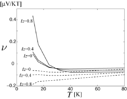
Figure 17: The Nernst coefficient $\nu$ with the CVC (solid line) and without the CVC (dotted line) for $t_{z}=0$, $0.4$, $0.8$ as a function of $T$ with $\alpha_{S}=0.995$ at $T=5$K

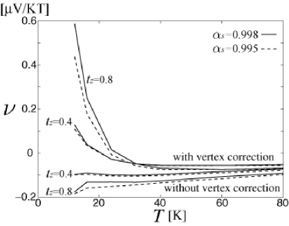
Figure 18: The Nernst coefficient $\nu$ with the CVC (upside) and without the CVC (downside) for $t_{z}=0.4$, $0.8$ as a function of $T$ with $\alpha_{S}=0.995$ (solid line) and $0.998$ (dotted line) at $T=5$K.

IV Conclusion

We have calculated microscopically the resistivity $\rho$, the Hall coefficient $R_{H}$ and Nernst coefficient $\nu$ for three-dimensional Hubbard model close to the AF QCP based on the Fermi-liquid theory. This is a first microscopic calculation for the Hall coefficient and the Nernst coefficient with the current vertex corrections (CVC) in the three-dimensional system. In two-dimensional systems, it is established that the CVC plays an important role when the AF fluctuations are strong. On the other hand, the CVC vanishes completely in infinite dimension $d=\infty$. Thus, it is a very important theoretical issue to clarify whether the CVC is significant or not in three-dimensional systems. We find that the CVC influences crucially on various transport phenomena in both two and three-dimensional systems close to the AF QCP.

We have shown that the magnitude of $R_{H}$ and $\nu$ is strongly enhanced with the decrease of temperature due to the CVC. These strong temperature dependences in the Hall coefficient and the Nernst coefficient come from the difference between the direction of the total current $(\mbox{\boldmath$J$}_{\mbox{\scriptsize\boldmath$k$}})$ and that of $\mbox{\boldmath$v$}_{\mbox{\scriptsize\boldmath$k$}}$ around the cold spots. The difference of directions increases as the temperature decreases near the QCP, which can be expressed in terms of the effective curvature $\partial\theta_{\mbox{\scriptsize\boldmath$J$}}/\partial k_{\parallel}$ of Fermi surface obtained by the direction of $\mbox{\boldmath$J$}_{\mbox{\scriptsize\boldmath$k$}}$. The obtained values of $R_{H}$ at the lowest temperature ($T=0.02$) is more than $5$ times larger than those at high temperatures for three-dimensional system ($t_{z}=0.8$). This result is qualitatively consistent with experimental results in various three-dimensional heavy fermion systems close to the AF QCP, such as CeCoIn₅ and CeCu_6-xAu_x. This strong enhancement cannot be explained by the relaxation time approximation (RTA).

In the present paper, we also studied the momentum dependence of relaxation time in three-dimensional systems due to strong AF spin fluctuations. In two-dimensional systems, it is known that hot spots and cold spots take line structures along $z$ axis, as the systems approach to the AF QCP. In three-dimensional systems, we find that hot spots become point-like (“hot points”) while the cold spots remain to take line structures (“cold lines”). The emergence of hot points and cold lines is expected to be general in three-dimensional systems close to the AF QCP. Transport phenomena are mainly determined by the cold spots. The area of cold spots in the phase space plays an important role. We find that the CVC around cold spots produces strong enhancement of $R_{H}$ and $\nu$. We emphasize that the strong enhancement of $R_{H}$ and $\nu$ comes from the effective curvature of the Fermi surface, $\partial\theta_{\mbox{\scriptsize\boldmath$j$}}/\partial k_{\parallel}$, enhanced by the CVC on cold lines, as shown in Fig. 12. Note that obtained results for $R_{H}$ and $\nu$ without the CVC, which corresponds to the RTA, are almost temperature independent.

In future, we will perform a quantitative study for the transport phenomena in CeCoIn₅ and CeRhIn₅, using a realistic band structure predicted by band calculations.mae ; har In the present paper, signs of $R_{H}$ and $\nu$ are opposite to actual experimental results. We expect that this discrepancy can be resolved by taking into account a proper band structure.

V ACKNOWLEDGMENTS

This work was supported by a Grant-in-Aid for 21st Century COE “Frontiers of Computational Science”. Numerical calculations were performed at the supercomputer center, ISSP. The authors are grateful to K. Yamada, J. Inoue, N. Nagaosa, Y. Matsuda, Y. Suzumura, D. Hirashima, Y. Nakajima and K. Tanaka for useful comments and discussions.

References

- (1) C. Petrovic, P. G. Pagliuso, M. F. Hundley, R. Movshovich, J. L. Sarrao, J. D. Thompson, Z. Fisk and P. Monthoux, J. Phys. Condens.: Matter 13, L337 (2001).
- (2) Y. Nakajima, K. Izawa, Y. Matsuda, S. Uji, T. Terashima, H. Shishido, R. Settai, Y. Onuki and H. Kontani, J. Phys. Soc. Jpn. 73, 5 (2004).
- (3) R. Bel, K. Behnia, Y. Nakajima, K. Izawa, Y. Matsuda, H. Shishido, R. Settai and Y. Onuki, Phys. Rev. Lett. 92, 217002 (2004).
- fuk (a) T. Fukuhara, H. Takashima, K. Maezawa and Y. Onuki, unpublished.
- (5) S. Paschen, T. Lühmann, S. Wirth, P. Gegenwart, O. Trovarelli, C. Geibel, F. Steglich, P. Coleman and Q. Si, Nature 432, 881 (2004).
- (6) B. P. Stojković and D. Pines, Phys. Rev. B 55, 8576 (1997).
- (7) A. Rosch, Phys. Rev. B 62, 4945 (2000).
- (8) R. Hlubina and T. M. Rice, Phys. Rev. B 51, 9253 (1995).
- ong (a) J. M. Harris, Y. F. Yan, P. Matl, N. P. Ong, P. W. Anderson, T. Kimura and K. Kitazawa, Phys. Rev. Lett. 75, 1391 (1995).
- (10) Y. Ando and T. Murayama, Phys. Rev. B 60, R6991 (1999).
- kon (a) H. Kontani, J. Phys. Soc. Jpn. 70, 1873 (2001).
- (12) E. H. Sondheimer, Proc. R. Soc. London, Ser. A 193, 484 (1948).
- mor (a) T. Moriya, Y. Takahashi and K. Ueda, J. Phys. Soc. Jpn. 59, 2905 (1990).
- (14) K. Ueda, T. Moriya and Y. Takahashi, J. Phys. Chem. Solids 53, 1515 (1992).
- mor (b) T. Moriya and K. Ueda, Adv. Phys. 49, 555 (2000); Rep. Prog. Phys. 66, 1299 (2003).
- bic (a) N. E. Bickers, D. J. Scalapino, and S. R. White, Phys. Rev. Lett. 62, 961 (1989).
- bic (b) N. E. Bickers and D. J. Scalapino, Ann. Phys. (N.Y.) 193, 206 (1989).
- (18) P. Monthoux and G. G. Lonzarich, Phys. Rev. B 59, 14598 (1999).
- kon (b) H. Kontani, K. Kanki and K. Ueda, Phys. Rev. B 59, 14723 (1999).
- kon (c) H. Kontani, J. Phys. Soc. Jpn. 70, 2840 (2001).
- kon (d) H. Kontani, Phys. Rev. Lett. 89, 237003 (2002).
- kon (e) H. Kontani and H. Kino, Phys. Rev. B 63, 134524 (2001).
- kot (a) A. Georges, G. Kotliar, W. Krauth and M. J. Rozengerg, Rev. Mod. Phys. 68, 13 (1996).
- kot (b) G. Kotliar and D. Vollhardt, Phys. Today 57, 53 (2004).
- (25) S. Koikegami, S. Fujimoto, and K. Yamada, J. Phys. Soc. Jpn. 66, 1438 (1997).
- kon (f) H. Kontani and K. Ueda, Phys. Rev. Lett. 80, 5619 (1998).
- bay (a) G. Baym and L. P. Kadanoff, Phys. Rev. 124, 287 (1961).
- bay (b) G. Baym, Phys. Rev. 127, 1391 (1962).
- (29) G. M. Eliashberg, Zh. Éksp. Teor. Fiz. 41, 410 (1961) [Sov. Phys. JETP 14, 886 (1962)].
- (30) H. Kohno and K. Yamada, Prog. Theor. Phys. 80, 623 (1988).
- (31) G. D. Mahan, Many-Particle Physics, 2nd ed. (Plenum Press, New York, 1990).
- kon (g) H. Kontani, Phys. Rev. B 67, 014408 (2003).
- (33) N. D. Mermin and H. Wagner, Phys. Rev. Lett. 17, 1133 (1966).
- (34) T. Ebihara, N. Harrison, M. Jaime, S. Uji and J. C. Lashley, Phys. Rev. Lett. 93, 246401 (2004).
- mor (c) T. Moriya and T. Takimoto, J. Phys. Soc. Jpn. 64, 960 (1995).
- (36) J. Takeda, T. Nishikawa and M. Sato, Physica C 231, 293 (1994).
- (37) Y. Ōnuki, R. Settai, K. Sugiyama, T. Takeuchi, T. C. Kobayashi, Y. Haga and E. Yamamoto, J. Phys. Soc. Jpn. 73, 769 (2004).
- (38) T. Maehira, T. Hotta, K. Ueda and A. Hasegawa, J. Phys. Soc. Jpn. 72, 854 (2003).
- (39) Y. Haga, Y. Inada, H. Harima, K. Oikawa, M. Murakawa, H. Nakawaki, Y. Tokiwa, D. Aoki, H. Shishido, S. Ikeda, N. Watanabe and Y. Onuki, Phys. Rev. B 63, 060503(R) (2001).
- fuk (b) H. Fukuyama, H. Ebisawa and Y. Wada, Prog. Theor. Phys. 42, 494 (1969).
- ong (b) Y. Wang, Z. A. Xu, T. Kakeshita, S. Uchida, S. Ono, Y. Ando and N. P. Ong, Phys. Rev. B 64, 224519 (2001).
- ong (c) Z. A. Xu, N. P. Ong, Y. Wang, T. Kakeshita and S. Uchida, Nature (London) 406, 486 (2000).
- kon (h) H. Kontani and K. Yamada, J. Phys. Soc. Jpn. 74, 155 (2005).
- (44) R. Settai, H. Shishido, S. Ikeda, Y. Murakawa, M. Nakashima, D. Aoki, Y. Haga, H. Harima and Y. Ōnuki, J. Phys.: Condens. Matter 13, L627 (2001).
- (45) Y. Nishikawa, H. Ikeda and K. Yamada, J. Phys. Soc. Jpn. 71, 1140 (2002).